|
Pesticides Research no. 86, 2004 Fate of Pyrethroids in Farmland PondsContentsPART I : Fate of pyrethroids in farmland ponds. Field studies 5 Materials and methods, part I
6 Results and discussion, part I PART II : Fate of pyrethroids in farmland ponds. Experimental data interpretation using mathematical models 9 Aim and solution strategy, part II 10 Physicochemical characteristics, part II 11 Experimental results, part II 12 System description, part II 13 Model formulations, part II
14 Sediment/water system analysis, part II
15 Surface micro layer, part II 1 PrefaceThis report is a part of the research programm "Effects of Pesticides on Ponds". The projects were funded by the Danish Environmental Protection Agency' s Research programme on Environmental effects of pesticides. The aim of the project was: To develop a model-based tool for evaluation of risk related to pesticide exposure in surface water. The tool must be directly applicable by the Danish Environmental Protection Agency (DEPA) in their approval procedure. As part of this goal, the project had to:
The project consisted of four subprojects with individual objectives. The sub-projects are listed in Table 1. Table 1. Sub-projects of " Effects of Pesticides on Ponds". Tabel i. Oversigt over delprojekter i "Effekter af pesticider i vandhuller".
The reports produced by the projects are:
The project was overseen by a steering committee. The members have made valuable contributions to the project. The committee consisted of:
The authors want to thank the following technicians at NERI, Department of Environmental Chemistry, for their enthusiasm during the project: Jørgen Holst, Niels Axel Sommer, Marianne Reni Olsen, Bjørg Lindblom and Dorte Thil Hansen. They have done a tremendous work including keeping the ponds, spraying, sampling and analysing the samples. We thank Jim Huckins at the United States Geological Survey, Biological Resources Division, Columbia, Missouri for his advice on Semipermeable membrane devices and we thank Karsten Liber, University of Saskatchewan for fruitful discussions on design of mesocosm studies. 2 SummaryPart IPyrethroids constitute a group of insecticides, which have been used widespread in Danish agriculture. They are toxic to aquatic organisms. The aim of the present study has been to investigate the fate of these compounds in ponds in agricultural areas. A pond is a complex ecosystem. It can be considered to consist of a series of compartments. It was intended to investigate all compartments that are important either to the mass balance because they are place of residence for aquatic fauna. The most important compartments of pond ecosystems were a priori selected to be surface microlayer, water column and sediment. Concentration of dissolved pesticide in the water phase was studied by aid of semipermeable membrane devices (SPMDs). The fate of 4 pyrethroids, fenpropathrin, permethrin, esfenvalerate and deltamethrin was studied during a 2-year period. The results have been used to validate a distribution model and the model analysis has been used for interpretation of the pesticide measurements. The model analysis is published as part II of this report. The experimental ponds are artificial and have as far as possible been established to resemble natural ponds. The artificial ponds can unlike natural ponds be experimentally exposed to pesticides. The pesticides have been sprayed onto the pond surface. Samples of surface microlayer, water column and sediment have been collected and analysed from 1 hour after spraying to 8-16 days after spraying with increasing intervals. In surface microlayer is the concentration of pesticides initially very high because that is where the pesticides enter the ponds. The concentration drops quickly because of mixing into the rest of the water compartment. The concentration of pesticides is however, 8-10 times higher in the surface microlayer compared to the water phase throughout the observation period. In the water phase the pesticides become evenly distributed within the first day after spraying. The concentration drops quickly, mainly because the pesticides are adsorbed to the sediment particles. Permethrin, esfenvalerate and deltamethrin rearrange into other isomers in the surface microlayer and the water column. Concentrations of pesticides in the SPMDs reflect the concentration profile of dissolved pesticides in the water column. The dissolved pesticide is bioavailable. Model analysis has demonstrated that pyrethroids are adsorbed in the upper few mm. of the sediment. Part IIThe focus in this report is on the mechanisms governing pyrethroid exposure in small farmland ponds. Experimental results in form of time series of pesticide concentration values are interpreted in a model analysis using mathematical models. The experiments are reported in detail in part I. Known doses of the active ingredients deltamethrin, permethrin, fenvalerate and fenpropathrin are spread at the surface of artificial ponds. In both the year 1995 and year 1996 spraying experiments have been undertaken in two ponds. All four pyrethroids were out sprayed in each experiment. However, only the fenpropathrin measurements were valid for 1995, in relation to mathematical model interpretation, due to analytical problems. Different compartments in the ponds were measured and mainly results from the water column and surface micro layer are used in this analysis. The experimental results from the artificial ponds are supplied by laboratory experiments using small glass containers (Morgenroth, 1992a and b). The purpose of the mathematical model analysis is to identify the most realistic model which can explain the experimental results. Furthermore, the models can help to generalise the experimental results to conditions different from the test conditions. A paradigm for selecting the model structure is suggested, where two statements are used: (1) the model shall be able to describe the experiment, and (2) the model structure shall be as simple as possible. The first statement is obviously necessary and the last statement is needed in order to avoid suggestions of models of unnecessary high complexity. Such over-complex models may describe the experiment but the suggested model structure can easily be misleading. This analysis is based on a kind of catalogue of possible mechanisms taking place in the pond. Different realistic combinations from this catalogue forms a series of alternative models having different levels of complexity. The task is now to select the least complex model, which can describe the experiment. An idealised pond system is defined consisting of air, water column and sediment sub systems, where substance is transmitted between the different sub systems. The water column is assumed completely mixed having no concentration gradient from top to bottom, which is shown to be valid a few hours after spraying (part I). The exchange of substance to the air is assumed to be a first order release to the air from the water column. The sediment is assumed to be homogenous, in which vertical one dimensional diffusion can take place from the water column and through a laminar boundary layer at the sediment surface. The substances adsorbed to the sediment solids are assumed to be in local equilibrium in relation to the substance dissolved in the pore water. Degradation is assumed to be a first order degradation in both the water column and the sediment. A specific model is suggested in relation to the surface micro layer in which diffusion, adsorption and first order volatilisation are included. It has not been possible to suggest a model for the surface micro layer. The data are too limited and knowledge about the 'real' layer thickness is missing. However, some negative conclusions can be drawn because a diffusion type model including the diffusion through the micro layer, linear adsorption and 1. order volatilisation from the surface seems to release the substances from the micro layer too quickly. The measurement of surface micro layer concentrations seems very uncertain so the missing coincidence between model and experiment can be a result of either uncertainty in model assumptions or the uncertainty in the experimental result. For the sediment water column system the model including sediment pore water diffusion, linear adsorption to sediment solids and degradation in the sediment seem most promising. Both experiments in the artificial ponds and in the laboratory support this type of model. However, the degradation mechanism was not an important description for fenpropathrin which also seems to have higher sediment adsorption than the other substances. For deltamethrin, permethrin and fenvalerate there was a distinct difference between pond 3 and pond 4, which were replicates. The most probable explanation is the difference in biomasses due to a snail invasion in pond 3, which increased the adsorption mechanisms in pond 3, mainly due to the increased turbidity in water column caused by snail activity. Laboratory experiments for fenvalerate including sediment measurement show a transport into the sediment as predicted by the pond investigation for the other pyrethroids. Furthermore, sediment degradation is observed in the laboratory experiments from sediment contamination measurements. The sediment pore diffusion coefficient in the lab scale experiment is much smaller (60 fold) than the diffusion coefficient in the pond sediment. This indicates that the diffusion into the sediment in the pond is increased due to sediment heterogeneity. A generalised curve is constructed for fenpropathrin based on the suggested sediment/water column model. The model predicts the concentration to be proportional to the dosage and nearly independent of pond depth. This makes is possible to perform a generalised concentration time series for the water column which is independent of both dosage and depth. The tendency of independence between depth and concentration levels seems to be a result of the quick and concentration dependent disappearance from the water column. Therefore, all hydrophobic substances will tend to have this type of independence when the initial concentration is formed as a surface area specific (atmospheric) deposition. The experimental result given in this analysis was not sufficient to make a clear distinction between the diffusion coefficient and the adsorption in the sediment. Only the product between the diffusion coefficient and the retention factor comes out of model calibrations. Therefore, additional adsorption tests using the sediment material will be beneficial in further experiments. The sediment water column model can be used in experimental design. Such an optimisation is outside of the scope of the present work, but it should be indented in planning of future experiments. The knowledge needed is the experimental error, the cost for sampling, analysing and spraying and the constrains in form of the number of ponds and the overall time schedule. Different experimental strategies can be tested to determinate the uncertainty of the process related parameters (degradation, adsorption, diffusion). The cost and the associated uncertainty can be estimated and the optimal combination identified. 3 SammendragDel IPyrethroider er en gruppe insekticider, som har været anvendt meget i dansk landbrug. De er giftige for vandorganismer. Formålet med nærværende undersøgelse har været at undersøge skæbnen af disse stoffer i markvandhuller. Et vandhul er et komplekst økosystem, som kan betragtes som sammensat af en række delelementer. Det var ønsket at undersøge alle delelementer, som er vigtige enten for massebalancen eller fordi de er levesteder for vandhulsdyrene. På forhånd blev følgende delelementer udpeget som vigtige: Overflademikrolaget, vandsøjlen og sedimentet. Lipidfyldte semipermeable membraner (SPMDer) blev anvendt til at undersøge koncentrationen af opløst pesticid i vandfasen. I en 2-årig undersøgelse er skæbnen i vandhuller af 4 pyrethroider, fenpropathrin, permethrin, esfenvalerat og deltamethrin, blevet undersøgt. Resultaterne er blevet brugt til at validere en distributionsmodel, og modelanalysen er brugt til at tolke resultaterne af pesticidmålingerne. Modelanalysen udgør part II i denne rapport. Vandhullerne er kunstige vandhuller, som så vidt muligt er bragt til at ligne naturlige vandhuller. Vandhullerne kan i modsætning til naturlige vandhuller anvendes til forsøg med pesticider. Pesticiderne er blevet sprøjtet ud på overfladen af vandhullerne. Fra 1 time efter udsprøjtningen til 8-16 dage efter udsprøjtningen er der med voksende interval blevet taget prøver af overflademikrolag, vandsøjle og sediment, og koncentrationen af pesticider er blevet målt. I overflademikrolaget er koncentrationen af pesticider meget høj i starten, da det er der pesticiderne rammer vandhullet. Koncentrationen falder hurtigt som følge af opblanding i resten af vandfasen. Gennem hele forsøgsperioden er koncentrationen af pesticider i overflademikrolaget dog 8-10 gange højere end i vandsøjlen. Pesticiderne fordeler sig hurtigt i vandfasen, hvori koncentrationen hurtigt falder, først og fremmest fordi pesticiderne adsorberes til sedimentet. I overflademikrolaget og i vandfasen sker en omlejring af permethrin, esfenvalerat og deltamethrin til andre isomerer. Koncentrationen af pesticider i SPMDer afspejler koncentrationsprofilen af opløst pesticid i vandfasen. Det er det opløste pesticid, der er biotilgængeligt. Modelanalysen har vist, at pyrethroiderne adsorberes i de øverste få mm. af sedimentet. Del IIDenne rapport samfatter de forhold, der har betydning for pyrethroiders eksponering i vandhuller. Eksperimentelle resultater i form af tidsserier af pesticidkoncentrationer er tolket i modelanalyser med anvendelsen af matematiske modeller. De eksperimentelle resultater er detaljeret beskrevet i del I. Kendte doseringer af aktivstofferne deltamethrin, permethrin, fenvalerat og fenpropathrin er sprøjtet ud på overfladen af kunstigt anlagte damme. Sådanne eksperimenter er blevet udført i to vandhuller én gang hvert år i årene 1995 og 1996. Alle fire pyrethroider var udsprøjtet hver gang, men for år 1995 er det kun resultaterne for fenpropathrin, der kan anvendes i forbindelse med matematisk modellering. Dette skyldes analysetekniske problemer. Der blev målt på forskellige medier i vandhullerne og af disse var det især vandsøjlen, samt overflade mikro laget, der blev anvendt i modelanalyserne. De eksperimentelle resultater fra vandhullerne blev suppleret med laboratorieresultater, hvor der blev brugt små (1 liter) glasbeholdere (Morgenroth, 1992a og b). Formålet med den matematiske modelanalyse er identifikation af den mest realistiske model, der kan forklare de eksperimentelle resultater. Desuden kan modelleringen hjælpe med til at generalisere eksperimenterne til andre omstændigheder, end de opmålte. Identifikationen af den mest realistiske model tager udgangspunkt i et paradigma for modelvalg, hvor der indgår to kriterier: (1) modellen skal kunne beskrive de eksperimentelle resultater og (2) modelstrukturen skal være så simpel så mulig. Det første kriterie er oplagt, mens det andet kriterie er nødvendigt for at undgå modeller med unødvendig høj kompleksitet. Sådanne overkomplekse modeller kan måske nok beskrive eksperimenterne, men deres struktur kan blive vildledende eller direkte forkerte som forståelsesramme. Analysen er baseret på et slags katalog over mekanismer med en mulig relevans for stoffernes forekomst. Disse mekanismer er så kombineret på forskellig vis i en stribe af alternative modeller med forskellig kompleksitet. Målet er at udvælge den mindst komplekse model, der kan beskrive eksperimentet. Et idealiseret vandhulssystem er defineret som bestående af tre delsystemer: en atmosfære, en vandsøjle og et sediment delsystem, hvor stoffer transporteres mellem delsystemerne. Vandsøjlen er forudsat totalt opblandet med samme koncentration overalt i vandsøjlen, hvilket synes at være en gyldig forudsætning få timer efter udsprøjtning (del I). Udvekslingen af stoffer til luften er forudsat beskrevet ved en første ordens fjernelse fra vandsøjlen. Sedimentet er forudsat homogent, i hvilket en vertikal endimensional diffusiv transport kan foregå fra vandsøjlen og ned i sedimentet gennem det laminare grænselag mellem vandsøjle og sediment. Stof adsorberet til strukturen i sedimentet er forudsat i lokal lineær og reversibel ligevægt i forhold til stof opløst i porevandet. Der er forudsat første ordens nedbrydning i både vandsøjlen og sedimentets porevand. En specifik model er foreslået for overflademikrolaget, i hvilken diffusion, adsorption og første ordens nedbrydning og afdampning er inkluderet. Det var ikke muligt at finde en rimelig overbevisende overensstemmelse mellem model og de eksperimentelle resultater for overflademikrolaget. Datagrundlaget var for spinkelt og den reelle mikrolagstykkelse var ukendt. Der kan dog drages nogle negative konklusioner fordi modellen syntes at afgive stof til den underliggende vandsøjle for hurtigt. Målingerne af koncentrationen i overflademikrolaget er behæftet med stor usikkerhed, hvorved den manglende overensstemmelse mellem model og eksperiment kan skyldes usikkerhed i modellen såvel som i eksperimentet. For systemet med vandsøjle og sediment var den mest overbevisende model den, der inddrog diffusion og adsorption, samt nedbrydning i sedimentet. Både eksperimenterne i vandhullerne og i laboratoriet pegede mod dette resultat. For fenpropathrin var det dog ikke muligt at identificere nogen betydende nedbrydning. Fenpropathrin synes at have en større adsorption til sedimentet end de andre stoffer. For deltamethrin, permethrin og fenvalerat var der en tydelig forskel mellem to vandhuller, der ellers var replikater. Den mest sandsynlige forklaring på dette er en snegleinvasion i den ene vandhul, hvilket øgede adsorptionen i vandsøjlen i dette vandhul, primært som et resultat af en øget turbiditet (svæv), der skyldtes sneglenes aktivitet. Laboratorieeksperimenter for fenvalerat, der både indeholdt målinger fra vandsøjle og fra sediment, viste at stof blev transporteret ned i sedimentet på samme måde som i vandhullerne. Desuden blev nedbrydningen i sedimentet direkte observeret i laboratoriet vha. målingerne af sedimentets stofindhold. Den kalibrerede diffusionskoefficient i sedimentporerne i laboratorieeksperimentet var dog 60 gange mindre end den tilsvarende kalibrerede koefficient i vandhullerne. Dette indikerer at diffusionen ned i sedimentet i vandhullerne er øget pga. heterogenitet i det naturligt dannede sediment. En generaliseret tidskurve kan konstrueres for fenpropathrin baseret på den foreslåede sediment/vandsøjle model. Modellen forudsiger at koncentrationen vil være proportional med doseringen og næsten uafhængig af dybden. Dette muliggør konstruktion af en generaliseret koncentrations tids kurve, som er uafhængig af dosis og dybde. Fra denne kan en vilkårlig koncentration til en vilkårlig tid bestemmes for en vilkårlig dosis og dybde. Det faktum at koncentrationen synes uafhængig af dybden er blot et resultat af den hurtige, men koncentrationsafhængige forsvinden fra vandsøjlen. Det betyder at alle hydrofobe stoffer, der hurtigt optages i sedimentet og som bliver sprøjtet ud på overfladen vil udvise den samme tendens for uafhængighed mellem vanddybde og koncentrationsniveau i vandsøjlen. De eksperimentelle resultater var ikke tilstrækkelige til at give en klar skelnen mellem adsorption og diffusion i sedimentet. Kun produktet mellem diffusionskoefficienten og retentionsfaktoren, kan bestemmes ved modelkalibrering. Derfor bør fremtidige eksperimenter udvides til at indeholde egentlige adsorptions test med anvendelse af det aktuelle sediment hvor adsorptionskoefficienten bestemmes uafhængigt af diffusionskoefficienten. De udviklede modeller kan anvendes for eksperimentel design af kommende eksperimenter. Sådanne optimeringer er ud over rammerne for denne undersøgelse, men det bør anvendes i planlægningen af nye eksperimenter. Den nødvendige viden er kendskab til de eksperimentelle fejl (både prøveindsamling, -håndtering og analyse), kendskab til priser for prøvehåndtering og analyse, samt bindinger i forhold til tidsrammer og antallet af disponible vandhuller. Forskellige strategier kan testes i en usikkerhedsanalyse, hvor de kendte usikkerheder lægges ind i modellen og usikkerheden på de kalibrerede parametre (f.eks. diffusionskoefficienten i sedimentet) bestemmes. Priser og usikkerheder kan derved sammenkobles og den optimale strategi vælges, hvor der kommer den mest præcise information ud af eksperimentet til en given pris. PART I : Fate of pyrethroids in farmland ponds. Field studies4 Introduction, part IMany pesticides, especially insecticides, are toxic to aquatic life. During application of pesticides they may accidentally reach streams and ponds e.g. by wind drift. To assess potential harm from pesticides to aquatic organisms in farmland ponds it is essential to know the fate of the pesticides in such ponds. Pyrethroid insecticides have been used widespread in Danish agriculture and they are very toxic to fish, crustacea and aquatic insects. For risk assessment purposes it is therefore important to know the distribution of these compounds in an aquatic ecosystem and their residence time in different parts of the system. The aim of this study is to investigate the fate of pyrethroid insecticides in small farmland ponds after the pesticides have been applied to the surface of the pond. This includes distribution in the pond, disappearance and bioavailability. The data generated are used to validate a distribution model. Since pyrethroids are used widespread in Danish agriculture and are relatively persistent in the sediment, the use of natural ponds of the farmland was not considered appropriate. Also since the biological community would be targeted during the experiment it was chosen to establish artificial experimental ponds. Four ponds of size comparable to smaller ponds in a Danish moraine landscape were excavated in a clay layer. Sediment was established by introducing a layer of topsoil on the bottom of the ponds and on the top of that a layer of sediment from a natural pond. From the natural pond was further transferred some macrophytes. The ponds filled with water during a winter season. From the natural sediment and from immigration a community of various species of plants and animals developed to form an ecosystem. During the experimental period we measured a series of water quality parameters in order to make sure that the condition of the ponds was close to the condition in natural ponds. An ecosystem is a complex system built up by biotic and non-biotic elements. To model a system it is necessary to divide it into compartments. This distribution model should include all compartments that are important either because they contribute significantly to the mass balance and/or because they are important as residence for sensitive aquatic organisms. The most important compartments of pond ecosystems were a priori selected to be:
Passive sampling of pyrethroids was carried out by aid of semipermeable membrane devices (SPMDs). SPMDs are layflat polyethylene tubes surrounding a neutral lipid (triolein). Uptake of lipophilic compounds into the membranes mimics uptake in aquatic organisms and the uptake may also give a possibility to estimate the concentration of dissolved pesticide in the water phase. The investigation is reported in two parts. The first part includes field studies while the second part focuses on the distribution model. 5 Materials and methods, part I
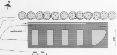
5.1 Establishing of experimental ponds, mesocosmsThe mesocosm facilities at NERI consist of four ponds with a bottom area of about 90 m2 and about 1 m's depth. The mesocosm facilities were established in November-December 1994. NERI is situated at the peninsula of Risø at Roskilde Fjord 8 km north of Roskilde, Sjælland, Denmark. The mesocosms are established in an area with heavy clay making it possible to retain water in the ponds without assistance of an artificial membrane. The excavation company Klingenberg in Roskilde carried out the excavation work. Consultant M.Sc. Lars Briggs, Amphiconsult, Fyn, gave advise on how to construct ponds and checked up on clay quality etc. The top soil was scraped into a bank 7 m south of the experimental area by the aid of a bulldozer revealing the clay. Excavators with caterpillar excavated 4 ponds and a larger reservoir. Size, cross section and mutual position of the ponds are shown in figures 5.1-5.2. A 1 m area along the four sides of each pond was left open. Outside this area the clay was piled to form banks around and between the ponds with an opening in the north bank for transport of equipment. Experimental ponds
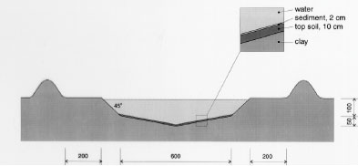
Figure 5.1 Oversigt over forsøgsarealet ved DMU, Roskilde, som viser de 4 vandhuller og reservoiret. Alle mål er i cm. Vandhullerne er nummereret fra 1 til 4 med vandhul 1 nærmest ved reservoiret. Skids were made in the short north sides of the embankments to facilitate transport of the sampling boat from one pond to another. A pipe from each pond leads to a ditch outside the bank. In case of surplus rainfall it is possible to adjust the water level in all ponds to 1.5 m by draining surplus water into the ditch. To initiate a sediment, the bottom of the ponds was carpeted with 10 cm of top soil. From a natural pond in a field near Svogerslev, in a landscape similar to Risø, natural sediment was sucked into a sludge tank and carried to the mesocosms. The sludge was uniformly sprayed unto the bottom of the ponds in a layer of about 2 cm. The natural sediment was introduced in order to initiate aquatic flora and fauna in the ponds.
Figure 5.2 Tværsnit af et vandhul, som viser udgravningsprofilen. Alle mål er i cm. During the winter precipitation filled the ponds and during the summer a good variety of plants, crustaceans and insects developed creating an ecosystem resembling the ecosystem of a natural pond. The banks and the walking area was sown with grass to prevent soil erosion. A grid system was indicated with numbered sticks every 2 m along the banks. A reservoir was excavated east of the ponds. Water from the reservoir can be used for additional supply of water to the ponds and for mixing of water from the different ponds in order to retain comparable initial conditions in the ponds. Water can be pumped from the ponds to the reservoir and back into the ponds. The first spraying with pesticides took place in September 1995 5.2 Spraying methodSpraying boom A special equipment has been constructed to make it possible to spray pesticides uniformly upon the water surface. The company OB Teknik in Dalmose, Denmark constructed a 8 m long spraying boom made of stainless steel. A steel pressure bottle contains the pesticide solution. Compressed air from another pressure bottle drives pesticide solution into the spraying boom from both sides, which reduces problems with drop of pressure along the boom. Nozzles 1553-08 from Hardi International were used to disperse the pesticides. Two-three persons carry the spraying boom and the steel bottles during spraying. The amount of pesticide sprayed pr. ha. is depending on the air pressure and walking speed. At a pressure of 2.5 bar the amount of spraying liquid was 5 L per 50 seconds. 5.3 Choice of pesticidesAt each spraying event, four different pesticides were sprayed simultaneously or within an hour on the pond surface. This procedure does not mimic a normal agricultural practice. However, the objective of the experiment is primarily to study the general fate of the pesticides and to generate data for calibration of the distribution model, not to study effects to aquatic life. In order to improve the distribution model four pyrethroids were selected with a range of physical chemical properties. Properties of the pyrethroids are given in table 5.1 and structure formulas are given in figure 5.3. Table 5.1 Fysisk kemiske egenskaber af de udvalgte pyrethroider. Data er indsamlet fra The Pesticide Manual 1991(tal til venstre) henholdsvis 1997(tal til højre). (Worthing and Hance 1991 and Tomlin 1997).
It is difficult to measure the physical chemical properties accurately, which is illustrated by the discrepancies between data from 1991 and 1997 in table 5.1. Deltamethrin
(S)-α-cyano-3-phenoxybenzyl (1R)-cis-3-(2,2-dibromovinyl)-2,2dimethylcyclopropanecarboxylate Esfenvalerate
(S)- α-cyano-3-phenoxybenzyl (S)-2-(4-chlorophenyl)-3-methylbutyrate Fenpropathrin
(RS)-α -cyano-3-phenoxybenzyl 2,2,3,3-tetramethylcyclopropanecarboxylate Permethrin
3-phenoxybenzyl (1RS)-cis-trans-3-(2,2-dichlorovinyl))-2,2-dimethylcyclopropanecarboxylate Figure 5.3 Strukturformler for de udvalgte pyrethroider: Deltamethrin, esfenvalerat, fenpropathrin og permethrin. (Worthing and Hance 1991) The spraying liquid was prepared from 3 formulated products. Active ingredients are given in brackets: Decis from Hoechst (deltamethrin), Sumirody 10 FW from Du Pont (fenpropathrin) and Sumi-Alpha 5 FW from Du Pont (esfenvalerate). A formulated product with permethrin was not available, so the active ingredient was dissolved in Decis prior to dilution of the product with water. Formulated products were preferred because additives like solvents and surfactants may influence the behaviour of the active ingredients in the aquatic system. 5.4 Sampling methodSampling took place from a small aluminium boat. The boat was moved from one site to another by pulling it with ropes in order not to stir the water unnecessarily. Surface microlayer Surface microlayer, SML, was collected by the method of Garrett and Duce (1980) with a steel screen 50 cm x 50 cm, mesh 1.25 mm The screen was lowered vertically into the water, turned 90°C and raised horizontally through the surface microlayer. The surface tension of the SML causes the SML to be caught in the mesh. The SML was collected in Duran bottles by tilting the screen. Water samples Water samples were collected at different depth. Two silicone tubes were fitted into the cap of a 1L Duran bottle and bent down with a ring. The bottle was lowered into the water and at the desired depth the ring was released, the tubes would then straighten and the water enter the bottle through one tube while the air from the bottle would escape through the other tube. This avoids turbulence at the inlet tube. Sediment samples Sediment samples were collected differently the two experimental years. The first year we used Kajak tubes consisting of a plexi glass pipe mounted on a stick. One end was closed with a one way valve allowing air and water to pass when the tube was lowered through the water and drilled into the sediment. The other end was open and the edge cut on the slant to facilitate the drilling. After the tube had been drilled into the sediment, the tube was lifted up, the valve would close and the sediment core was placed on a piston. The sediment core was pushed out of the tube with the piston and the upper 2 cm was cut off and collected in aluminium trays. The second year macrophytes had developed to have a more dense root web making it difficult to sample sediment with Kajak tubes. In stead a conventional half-sphere grab was used: Grab samples were placed in a box and the upper two cm collected into aluminium trays. 5.5 Semipermeable membrane devices (SPMDs)Passive integrative samplers were used to mimic the uptake of pesticide by aquatic organisms. We used semipermeable membrane devices (SPMDs) as described by Huckins et al., 1997. A standard SPMD consists of a LPDE (low density polyethylene) thin-walled, layflat tubing manufactured without additives. The membrane is sealed in both ends. A sequestration phase consisting of large molecular weight non polar liquids is placed as a thin film inside the tubing. Only the dissolved part of organic pollutants will diffuse into the membrane. Standard configuration is : 2.5 cm by 91.4 cm layflat LPDE-tubes (75-90 μm wall thickness) containing 1 ml (0.915 g) of triolein (sequestration phase) as a thin film. Standard semipermeable membranes (Huckins et al., 1997) were attached to two steel rods with metal clips. The rods with membranes were stuck in the pond bottom before spraying. The rods were placed so that the membranes were kept stretched between the rods. The lowest membrane was situated right above the sediment and the others in increasing distance from the bottom. After spraying of the ponds two membranes were attached to the rods above the water surface. The position of membranes in each pond is stated in the result chapter. 5.6 Experimental designEach year (1995 and 1996) two ponds were sprayed with pesticides and one pond served as a control. To obtain most information from the experiments (Liber et al., 1992) we wanted to spray two different concentrations of pesticides. However, in 1996 water snails had invaded one of the experimental ponds by thousands, causing a change in water conditions in that pond. In 1996 we therefore decided to spray the same concentration in both ponds and see if the different conditions would influence the fate of pesticides. Sampling time It was expected that changes in distribution and concentration would occur at a higher rate immediately after application. After spraying, samples were collected after 1, 2, 4, 6, 24 h and 2, 5, 8, 16 d. Samples of SML, water from20 cm's depth and sediment were collected from each quarter of a pond and pooled. Additional samples were collected from the middle of the pond, so called "gradient samples", from SML, 3 depth of water and sediment. Semipermeable mem-brane devices (SPMDs) For in situ measurement of bioavailable concentrations of pyrethroids were used semipermeable membrane devices (SPMDs) 5.7 Spraying schemeSampling schemes were intensive in the first week after spraying and it was logistically impossible to operate two simultaneously sprayed ponds. The spraying of the experimental ponds was therefore carried out with one weeks intervals. 1995 The first year pond 3 was sprayed 27 September. The pesticides were applied in two turns. Sumirody 10 FW (fenpropathrin) and Sumi-Alpha 5 FW (esfenvalerate) were applied at 11.30 a.m. and Decis (deltamethrin) with permethrin dissolved in it was applied at 12.00 a.m. Pressure was 2.5 bar, spraying time 50 s and 47 s. which corresponds to application of approximately 5 L of spraying liquid. Pond 4 was sprayed 4 October at 10.00 a.m. Fenvalerate, fenpropathrin, permethrin and deltamethrin were dissolved in Decis. All 4 pyrethroids were applied simultaneously. Pressure 2.5 bar, spraying time 49 s. corresponding to application of approximately 5 L of spraying liquid. 1996 The second year pond 3 and 4 were sprayed with the same dosage of pesticides and all four pyrethroids were sprayed simultaneously. Permethrin was dissolved in Decis, and this solution was mixed with Sumirody 10 FW and Sumi-Alpha 5 FW. Pond 4 was sprayed 12 June at 9.25 a.m. Pressure 2,5 bar. Spraying time 49s. corresponding to application of approximately 5 L of spraying liquid. Pond 3 was sprayed 19 June at 9.25 a.m. Pressure 2.5 bar. Spraying time 49s. corresponding to application of approximately 5 L of spraying liquid. Tables 5.2 and 5.3 show composition of the spraying liquid and the approximate application rate. Table 5.2 Koncentrationen af pyrethroider i sprøjtevæsken for hvert år og vandhul.
With a depth of about 75 cm, the size of the pond surface is about 7,5 times 17,5 m2, which is about 130 m2, and approximately 5 L of spraying liquid was applied. Table 5.3 Mængden af pyrethroid der er udsprøjtet på overfladen af vandhullerne, mg/m2
5.8 Handling and preservation of samplesIn the field Immediately after sampling the samples were placed in a thermo-box with freeze elements and stored there during fieldwork and transportation to the laboratory (2-4 hours). Preservation of samples in the laboratory After transfer of the samples to the laboratory they were all preserved according to the methods mentioned below. Sediment Sediment samples were frozen in the aluminium trays. SML and water samples SML and water samples for pesticide analysis: Recovery standard and isooctane were added to each bottle. The bottles were shaken and stored in a cold room at 4°C until time of analysis. Side parameters Samples for analysis of total-N and total-P were frozen. Samples for other side parameters were analysed the same day. SPMDs SPMDs were packed separately in aluminium foil and kept frozen until dialysis took place. 5.9 Analytical methods, pyrethroids5.9.1 ReagentsIsooctane p.a. (Merck, Germany), acetone glass distilled (Rathburn, UK), acetonitrile LiChrosolv 99.8% (Merck), dichloromethane HPLC glass distilled grade (Rathburn, UK), cyclohexane HPLC grade (Rathburn, UK), methanol LiChrosolv 99.9% (Merck), hydrochloric acid p.a. for activation of copper (Merck), carbon dioxide for supercritical extraction SFE/SFC grade (Air Products and Chemicals Inc.), copper granulate 0.2-0.6 mm 99.8% (Riedel de Haën, Germany), anhydrous sodium sulphate was cleaned by soxhlet extraction for 24 hours with dichloromethane, glass beads for the SFE cryo trap. Standards Lambda-cyhalothrin (ICI, UK), esfenvalerate (Pestanal, Riedel de Haën), cypermethrin (Pestanal, Riedel de Haën), fenpropathrin 97% (Riedel de Hahn), deltamethrin 99% (Pestanal, Riedel de Hahn), permethrin 97% (Pestanal, Riedel de Hahn). 5.9.2 ApparatusSupercritical fluid extraction (SFE) Suprex SFE Autoprep 44TM, Suprex, USA, equipped with a cryo trap, a modifier pump and an auto sampling system for collection of eluate from the trap. GC-system Gas chromatograph, HP 5890 (Hewlett Packard, USA) equipped with an electron capture detector and automatic sampler HP 7673A. HP Chemstation from Hewlett Packard was used for controlling the GC program, collection of data and data analysis. Column was 5% phenyl methyl fused silica capillary column from J & W Scientific. Length 60 m, diameter 0.25 mm, film thickness 0.1 μm. HPLC-system Waters pump model 510, Waters WISP 712 autosampler, HPLC gel permeation column Phenogel 10μ particle size, 100 Å pore size from Phenomenex, 300 x 21.2 mm, with a Phenogel pre column 10 μ, 50x7.8 mm. Column thermostat was produced in NERI's work shop. 5.9.3 Sample preparationSurface microlayer and water samples Surface microlayer and water samples were solvent extracted three times with approximately 120 ml/L isooctane each time. The extracts were dried by passing through sodium sulphate, concentrated by rotorevaporation and the volume adjusted to 1 ml after addition of lambda-cyhalothrin as an internal standard. Sediment Sediment samples were sieved at 2 mm, freeze-dried and extracted by super critical fluid extraction (SFE). 3 g of dry sediment was placed in an extraction cell, 100 μl 1000 ng/ml cypermethrin standard was spiked on top of the sediment as a recovery standard and 2 g of activated copper granules was added on top to desulphurize the extract. Extraction conditions were 10 min. static and 25 min. dynamic extraction, flow 1.5 ml/min, pressure 350atm., temperature 50°C, modifier 5% acetone. Trap material glass beads, trap temperature 50°C, restrictor temperature 50°C, eluting temperature 50°C, eluent acetonitrile 3.6 ml. The eluate was evaporated with a nitrogen flow and redissolved in isooctane after addition of internal standard. SPMDs Semipermeable membranes were dialysed twice in 200 ml cyclohexane. 200 μl of recovery standard cypermethrin, 1000 ng/ml, was added to the dialysates prior to evaporation to about 200 μl in a rotorvapor system. Possible residues of triolein, oleic acid or other were separated from the analytes by size exclusion HPLC. Injection volume 600 μl. Eluent 2% methanol in dichloromethane, 4 ml/min. Fraction collection from 13.5 to 21 minutes in 50 ml flask. The eluate was evaporated almost to dryness. The analytes were transferred to a 1 ml flask with isooctane, internal standard lambda cyhalothrin was added and the volume adjusted to 1 ml. 5.9.4 Detection by GC analysisGC-analysis All samples were detected by GC-analysis. GC conditions were: Splitless injection, purge time 3 min, injection volume 1 μl, carrier gas helium at flow rate 1-1.5 ml/min, injection temperature 325°C. Temperature program: Initial temperature 105°C increasing with 15°C/min to 250°C and then with 1°C/min to 280°C and 15°C/ min to 295°C. Detector temperature was 300°C. 5.9.5 Quality controlWater and surface micro layer Two pond water samples spiked with the four pyrethroids and one unspiked (blind) were analysed parallel to each batch of water and surface microlayer samples. Pond water was taken from an untreated pond. Sediment Sediment from an untreated pond was sieved and freeze dried and spiked with the four pyrethroids dissolved in isooctane. The sediment was carefully mixed by rotation in a rotorvapor system at atmospheric pressure. After this isooctane was evaporated. Two spiked sediment samples and one unspiked (blind) were analysed parallel to each batch of sediment samples. 5.10 Side parametersThe physical state of the ponds was controlled during the experiments by measuring a number of parameters parallel to the pesticide analyses. Chlorophyll A Content of Chlorophyll A in water is a measure of phytoplankton biomass. Chlorophyll A was measured by the Danish Standard DS 2201 (1986) method. Samples were filtered the day the were collected, and the filters were frozen and analysed within 14 days. Alkalinity Alkalinity was detected by the titrimetric method DS 253 (1977). Nitrogen and phosphorus Total nitrogen and phosphorus content was detected by the methods DS 221 and DS (1975) and DS 292 (1985). Samples were frozen the day of collection and stored at -20°C. The analyses were carried out in 1997 at the Department of Fresh Water Ecology in Silkeborg. Oxygen In 1995 temperature and oxygen saturation was measured in situ with a probe. During the experiment the oxygen electrode turned out to be unstable and some of the data are not reliable. Temperature In 1995 water temperature at various depth was measured together with oxygen. pH pH was detected in the laboratory the same day with a pH meter. Turbidity, conductivity, salinity, pH, oxygen, temperature In 1996 a new probe: HORIBA water quality checker U-10 (Horiba, Japan) was applied for determination of temperature, turbidity, conductivity, salinity, pH and oxygen concentration, corrected for salinity, in situ. Texture analysis The Danish Institute of Agricultural Sciences, Research Centre Foulum, carried out texture analysis of sediment. 6 Results and discussion, part I6.1 Pyrethroids in pond samples6.1.1 IsomerisationAll the pyrethroids have asymmetric carbon atoms (figure 5.3) and therefore the compounds have the possibility of a number of different stereo isomers. The insecticidal activity of the isomers varies and in modern formulations it is often only the most active isomer that is present. This is e.g. the case with deltamethrin in Decis and esfenvalerate in Sumi-alpha. Permethrin is a mixture of cis and trans compounds and the ratio of isomers should be stated for every product. (Worthing and Hance 1991). The ratio of isomers in standard solutions in isooctane of the different pyrethroids is stable at laboratory conditions. However, it was observed during analysis of samples from the first experimental year that the ratio in pond samples changed during time, but these observations were not quantified. The second year the different isomers were quantified. Two permethrin stereo isomers are present in the standard compound and each isomer is quantified separately. In esfenvalerate and deltamethrin standards only one stereo isomer is present. Assuming that the GC-ECD response factor is the same for different isomers of the same compound it is possible to calculate the concentration of the various isomers by aid of the ratio of peak areas and the standard curve. Once isooctane has been added to samples of water and SML it seems to stabilise the isomer ratio because the pyrethroids are extracted into the isooctane. The isomerisation in the ponds is discussed below for water phase. Figures 6.1 – 6.3 demonstrate the development of the isomer ratio of permethrin, fenvalerate and deltamethrin. Permethrin One hour after application the ratio of cis-permethrin to trans-permethrin was about 0.70. This ratio increases during the observation time. After 5 days the ratio was about 1.5 and after 8 days it was about 5.5. The last point of observation is more uncertain because the concentration of trans-permethrin was very low. It is not obvious from the figures if equilibrium will be obtained. Esfenvalerate Esfenvalerate is (S)--cyano-3-phenoxybenzyl (S)-2-(4-chlorphenyl)-3-methylbutyrate. Fenvalerate is a mixture of (R) and (S) isomers with unstated stereochemistry. In the gaschromatogram fenvalerate is detected as two peaks, the second peak with same retention time as esfenvalerate. In esfenvalerate there will often be small amounts of the first peak present as well. Equilibrium was not obtained but it seems that the isomer ratio is approaching a constant value indicating that the isomerisation process is reversible. Deltamethrin Isomerisation of deltamethrin is very similar to the isomerisation of esfenvalerate.
Figure 6.1 Tidsafhængig forhold mellem de to permethrin isomerer i vandhulsvand
Figure 6.2 Tidsafhængig forhold mellem de to fenvalerat isomerer i vandhulsvand
Figure 6.3 Tidsafhængig forhold mellem de to deltamethrin isomerer i vandhulsvand 6.1.2 Surface microlayerAt the interface between air and water is a surface microlayer (SML). The SML contains humic substances, fatty acids and alcohol's, polysaccharide-protein complexes and other substances that exhibit surfactive properties. The concentration of bacteria and abiotic particles is 102-104 times the concentration in the water (GESAMP 1995). Peter Fatum (1996) made his master thesis at NERI in connection to this pond study. The thesis includes a survey of literature on SML to which we refer. The SML is not well defined and the thickness of the microlayer is in this investigation defined by the sampling method. Sample collection with a Garrett screen mesh 1.25 mm and size 0.25 m2 gave 85 ml of SML corresponding to a surface microlayer thickness of 0.34 mm. Theoretical initial concentration 5 L of spraying liquid was applied to a surface of approximately 130 m2 corresponding to 0.04 mm of liquid which is a minor size (12%) compared to the thickness of the SML. For calculation of a theoretical initial concentration of pesticide in the SML after spraying, it is anticipated that all the pesticide is present in the SML, the SML being defined by the sampling thickness as mentioned above. Theoretical sample volume of the SML is 130 x 10,000 x 0.034 cm3 = 44.2 L. The theoretical concentrations are shown in table 6.1 Table 6.1 Teoretisk startkoncentration af pyretroider i overflade mikrolaget (øverste 0,34 mm).
These concentrations are much higher than the solubility of these pesticides in pure water (table 5.1), but the solubility is increased by the presence of surfactants in the formulated pesticide products. Figures 6.4 - 6.5 show the concentration of pesticides in surface microlayer from 1 hour after spraying to 8 days after spraying .
Figure 6.4 Koncentrationen af pyrethroider i overflademikrolaget fra 1 time til 8 dage efter udsprøjtning. Vandhul 3 1995
Figure 6.5 Koncentrationen af pyrethroider i overflademikrolaget fra 1 time til 8 dage efter udsprøjtning. Vandhul 4 1995 It is seen from the figures, that the concentration of pesticides decreases very rapidly. After two hours the concentration of pesticide has declined to about 0,3-7% of the initial concentration as shown in table 6.2. Table 6.2 Koncentration af pyretroider i overflade mikrolaget to timer efter udsprøjtningen. Procentdel af den teoretiske startkoncentration. I 1996 er det summen af isomerer.
After one hour most of the decline is caused by diffusion from the SML into the water column and turbulent mixing within the water. The decline is faster in 1996, maybe caused by different climatic conditions. 6.1.3 Water columnDistribution Figures 6.6 – 6.9 show the concentration of fenpropathrin in the water column at three depths. The diagrams show examples of the course of concentration distribution and are illustrative for the other pyrethroids too.
Figure 6.6 Koncentrationsfordeling af fenpropathrin i vandhul 3 1995 1 til 192 timer efter udsprøjtningen. Gradient 1-3 angiver prøvetagningsdybden (10 cm og 30 cm under overfladen og 30 cm over bunden).
Figure 6.7 Koncentrationsfordeling af fenpropathrin i vandhul 4 1995 1 til 192 timer efter udsprøjtningen. Gradient 1-3 angiver prøvetagningsdybden (10 cm og 30 cm under overfladen og 30 cm over bunden).
Figure 6.8 Koncentrationsfordeling af fenpropathrin i vandhul 3 1996 1 til 192 timer efter udsprøjtningen. Gradient 1-3 angiver prøvetagningsdybden (10 cm og 30 cm under overfladen og 30 cm over bunden).
Figure 6.9 Koncentrationsfordeling af fenpropathrin i vandhul 4 1996 1 til 192 timer efter udsprøjtningen. Gradient 1-3 angiver prøvetagningsdybden (10 cm og 30 cm under overfladen og 30 cm over bunden). One hour after spraying the pesticides have already been mixed into all of the water column. However, there is a distinct decrease in concentration from the upper 10 cm (gradient 1) to 30 cm above the bottom (gradient 3). After 6 hours the concentration is equal throughout the water body. The pesticides have been adsorbed to sediment and therefor the overall concentration has decreased. Pesticides remaining in the water phase are evenly distributed. Disappearance Figures 6.10 – 6.12 show the rate of disappearance of pyrethroids in the water column 20 cm below the surface. If the disappearance is ruled by first order processes then
Ct = concentration at time t
Figure 6.10 Forsvindingsrate for pyrethroider i vandhul 3 lav dosering 1995
Figure 6.11 Forsvindingsrate for pyrethroider i vandhul 4 høj dosering 1995
Figure 6.12 Forsvindingsrate for pyrethroider i vandhul 3 1996
Figure 6.13 Forsvindingsrate for pyrethroider i vandhul 3 1996 for summen af isomerer. pe=permethrin, fe=fenvalerate, de=deltamethrin
Figure 6.14 Forsvindingsrate for pyrethroider i vandhul 4 1996 for summen af isomerer. pe=permethrin, fe=fenvalerate, de=deltamethrin Figures 6.10 – 6.12 show disappearance of the single isomers while figures 6.13 – 6.14 show the sum of the isomers. For fenpropathrin the curves are identical, as fenpropathrin does not change into other isomers. In 1995 the disappearance rate was fast in the beginning and slowed down after about one day. This may partly be caused by a fast disappearance by mixing into the rest of the water column and adsorption into the sediment. After full mixing the decrease in concentration is mainly ruled by suction into the sediment. This is in agreement with the observation that full mixing was achieved after about one day (cf. figures 6.6 – 6.7) In 1996 there was mixing after a few hours (cf. figures 6.8 – 6.9) and therefore the change in disappearance rate is seen after two hours. The difference between 1995 and 1996 may be caused by differences in climatic conditions the two years (Experiments took place in October 1995 and in June 1996) or by differences in the amount of macrophytes. According to the model analysis (part II) disappearance of pesticides from the water phase does not follow first order relationship, so we cannot expect a linear log disappearance rate. By comparing figure 6.12 and figure 6.13 it is seen that part of the disappearance of permethrin, esfenvalerate and deltamethrin is caused by isomerisation. Figure 6.13 indicates that the disappearance rate in pond 3 of fenpropathrin, fenvalerate and deltamethrin is about the same if we look at the sum of isomers. The disappearance rate of permethrin is higher which may be due to a higher photosensitivity of this compound (Leahey 1985). Leahey (1985) also mentions photoisomerisation of permethrin and deltamethrin. This study demonstrates, that this is also the case for esfenvalerate. The disappearance rate in pond 4 is faster for permethrin, fenvalerate and deltamethrin. This observation is discussed in more detail in section 6.1.7 on SPMDs. 6.1.4 Enrichment in the SMLPyrethroid insecticides have very low solubility in water (see table 5.1) and are easily dissolved in organic solvents. So it is likely, that the pyrethroids will show higher affinity to the SML with its higher content of fatty compounds and surfactants than to the water phase. Enrichment factor The ratio of pesticide concentration in the SML compared to water phase is called the enrichment factor, EF. Figures 6.15 – 6.16 show the enrichment of pyrethroids in the SML compared to water in 1995.
Figure 6.15 Berigelse af pyrethoider i overflade mikrolaget i vandhul 3, lav dosering. EF=berigelsesfaktoren.
Figure 6.16 Berigelse af pyrethoider i overflade mikrolaget i vandhul 4, høj dosering. EF=berigelsesfaktoren. Right after application the enrichment factor is very high but it is not really an enrichment but rather a reflection of the pesticides not being mixed into the water phase yet. The rapid decline in EF is primarily a result of mixing. As demonstrated in section 6.1.3 the mixing within the water column is completed after about one day in 1995. After about one day the EF has also reached a constant value of 8-10 in pond 3 and 5-10 in pond 4 1995. This factor expresses the actual enrichment. Fatum (1996) also confirms this: In a laboratory experiment SML spiked with esfenvalerate was added to a water phase with pond water. The two phases were partly mixed, so after 2 hours the enrichment, EF, was 2.3. After 72 hours the EF was 11.7 which is in good agreement with the field results from the pond study. 6.1.5 SedimentResults of the sediment analysis 1996 are shown in figures 6.17 – 6.18. Results from 1995 are similar. Figure 6.17 Koncentrationen af pyrethroider i sediment tørstof fra vandhul 3, μg/kg Figure 6.18 Koncentrationen af pyrethroider i sediment tørstof fra vandhul 4, μg/kg The results of the sediment analysis are confusing. It was expected that sediment concentrations would increase at the beginning of the experiment caused by adsorption of the hydrophobic pyrethroids to sediment particles. After some days we expected to see a small decline caused by microbial degradation of the pesticides. The results do not contradict this hypothesis, but the uncertainty of the results seems to be too large. The uncertainty is a sum of uncertainties from sampling of sediment and analysis of sediment. Spiked sediment samples were used as reference material. Two reference samples were analysed with each batch of samples. The variance between these samples is the overall variance of the method of analysis. At each sampling time sediment samples were collected from each of the four quadrants of a pond. Most of the samples were pooled before they were sieved, dried and analysed. However, some of the samples were analysed without pooling. The variance between these samples also includes variance of the sampling procedure and variance caused by inhomogenity of pesticide distribution. However, the two contributions cannot be distinguished. Variance of analysis method sm2 is calculated from the spiked sediment samples. Total variance st2 including sampling, inhomogeneity of sediment and analysis is calculated as the mean variance of 4 series of analysis of sediment, one from each pond at day 16. It seems that the size of the variance is depending on the concentration level, which is different in the spiked samples compared to the day-16 samples. There is no reason to expect different variances for the four compounds. For that reason all variances have been converted to the variance of a 10 μg/kg sample. The variance of sampling is calculated as the difference between st2 and sm2. Table 6.3 shows the variances for each pyrethroid. Table 6.3 Usikkerhed på sedimentanalyser. st2 er total varians af prøvetagning og analyse. sm2 er varians af den analytiske metode and ss2 er varians af prøvetagning, inhomogenitet af sediment o.s.v. Alle varianser er blevet omregnet til koncentrationen 10 μg/kg tør sediment.
The variances for fenpropathrin, permethrin and esfenvalerate are about the same. For deltamethrin it is somewhat higher. Re-examination of data from the spiked samples showed that in some samples the recovery of especially deltamethrin was poor, 15% and 21%, compared to usually 45%. The low recovery may come from the SFE extraction procedure, as it has later been observed that occasionally the amount of eluent has been too small, which will influence especially deltamethrin, which is eluted latest from the trap. It seems that contribution to variance (uncertainty) from sampling is about 5-10 times the contribution from analysis. According to the model analysis (part II) the pyrethroids are mainly adsorbed in the upper 1-2 mm of the sediment. We sampled approximately the upper 2 cm of the sediment for analysis. This has introduced some uncertainty in how much the contaminated sediment was diluted with uncontaminated sediment during sampling: Future analysis of pesticides in sediment will need improvement of sampling technique as well as extraction procedure. 6.1.6 SPMDsResults from SPMD experiments are available from 1996. Membranes were placed in the ponds immediately prior to spraying, except the membranes above the water surface, which were mounted one hour after spraying. The SPMDs were left in the ponds for two month. Figures 6.19 and 6.20 show the concentration of pyrehtroids in the membranes. Each value is the average of duplicate observations.
Figure 6.19 Indhold af pyrethroider, sum af isomerer, i SPMDer i vandhul 4, μg/membran.
Figure 6.20 Indhold af pyrethroider i SPMDer, sum af isomerer, i vandhul 3, μg/membran. Pond 4 is the pond with clear water while the water in pond three contained more particulate matter caused by the activity of the snails. Concentration of pesticides in membranes above the water surface was low compared to SPMDs exposed to water, the amount being 50-200 ng/-membrane. This amount reflects the concentration of pyrethroids in the air above the water. It is either the result of evaporation of pyrethroids or it may come from small droplets of spraying liquid remaining in the air. For fenpropathrin, permethrin and fenvalerate, the amount of pesticide uptake in the membrane is largest close to the surface. In pond 4 the concentration in SPMDs decreases with distance from the surface. In pond 3 there seems to be a fall in concentration from the surface to 20 cm below the surface and a small increase closer to the sediment. The concentration of deltamethrin in SPMDs is lower than that of the other pyrethroids especially in the upper part of the water column. The uptake of pyrethroids in the SPMDs depends on the concentration of dissolved compound in the water. Pesticide adsorbed to particulate matter or dissolved organic matter will not pass the membrane (Huckins et al., 1997). The concentration of a compound in the SPMDs results from a simultaneous uptake and elimination but for very hydrophobic compounds like the pyrethroids the elimination rate is very low. When SPMDs are exposed to solutions of lipophilic compounds the initial uptake will be linear. In the ponds there is a concentration gradient after spraying and this gradient levels out within about 4 hours. Within that period the uptake will still be linear. That means that the concentration of pesticide in the membranes reflects the maximum concentration of dissolved pesticide that the membranes have experienced during the exposure time. To calculate the concentration of a compound in the water, it is necessary to know the uptake rate of the compound. This can be determined in laboratory experiments. This has not been done yet so the following interpretation of the data is only qualitative. The interpretation is supported by the model analysis in part II. The two ponds have received the same amount of pesticide and the same amount of each of them. If the two ponds were identical we would therefore expect the same concentration of pyrethroids in SPMDs from the two ponds. This is not the case. If the pyrethroids had the same physical chemical properties we would also expect the same concentration of each pesticide in the membranes. This is not the case either. The maximum concentration of pyrethroids in the SPMDs is much higher in pond 4. That may be explained by the presence of higher amounts of particulate matter in pond 3. Part of the pyrethroids will adsorb rapidly to the particulate matter and thereby the concentration of dissolved pyrethroid is lowered. The pyrethroids adsorb strongly to the sediment, which sucks dissolved pyrethroid from the water causing a decrease in concentration in the water column. This decrease is faster in pond 4 cf. figures 3.10 and 3.11, which may again be explained by the increased retention of pyrethroids caused by adsorption to organic matter. The faster decrease in pond 4 is reflected in a steeper gradient in SPMD concentration in that pond. According to the model analysis this adsorption is reversible. Because of the delayed transport into the sediment, the concentration of pyrethroid is higher in pond 3 after some time. This is reflected in the higher concentration of pyrethroids in SPMDs in pond 3 apart from the initial uptake in the SPMDs at the upper position (75 cm from the bottom). Deltamethrin shows a quite different uptake pattern compared to the other pyrethroids. More experiments are needed to explain the difference. 6.2 Side parameters6.2.1 Chlorophyll AConcentration of chlorophyll A in subsurface pond water (20 cm) is shown in figures 6.21 and 6.22. Chlorophyll A is an indicator of phytoplankton growth. 1995 In 1995 the concentration of chlorophyll does not change much during the experiment except on September 28, where the concentration rises significantly in pond 2 (control) and pond 3 (low dosage). The samples were collected at the same time of the day as the other days so the light intensity is probably the same. The phenomenon is probably not caused by the pesticides since it is observed in the control pond as well.
Figure 6.21 Koncentration af klorofyl A i vandhulsvand 20 cm under vandoverfladen. År 1995, prøvetagningsdatoer er angivet som måned, dag. 1996 In 1996 pond 3 was dominated by big fresh water snails, which had eaten almost all the macrophytes. This implied a totally different environment compared to pond 2 and 4. From figure 6.22 it is seen that chlorophyll concentration in pond 2 and 4 is at the same level of 2-4 μg/L throughout the experiment. However, in pond 3 the chlorophyll concentration increases up to 15 μg/L with the increase beginning at day 1 after spraying. The algae bloom that is reflected by the concentration of chlorophyll may be caused by the lack of macrophytes thereby giving less competition to the algae for light and nutrients. At the same time most grassers like daphnia have been killed by the pyrethroids.
Figure 6.22 Koncentration af klorofyl A i vandhulsvand 20 cm under vandoverfladen. År 1996, prøvetagningsdatoer er angivet som måned, dag. 6.2.2 Other side parametersAlkalinity and conductivity were very stable for each pond throughout the season but changed a little from year to year. Table 6.4 shows the average values. In 1996 before spraying of pond 4, water from the three ponds were mixed together with ground water and water from the reservoir and pumped back to the ponds. Table 6.4 Ledningsevne og alkalinitet af vandhulsvand, gennemsnitsværdier og standard afvigelse.
Mean alkalinity of Danish lakes (Jensen et al., 1997) is 2.08 meq/L with 1.25 meq/L as the 25% fractile and 2.85 as the 75% fractile. Alkalinity of the pond water seems to cover a broad range of Danish lakes. Figures 6.23 – 6.25 show variation of O2 concentration, temperature, pH and turbidity of the pond water in 1996. 1995 Figure 6.23 Målte værdier af opløst O2 koncentration, temperatur, pH og turbiditet i vandhul 4 fra 12 juni til 28 juni 1996. Figure 6.24 Målte værdier af opløst O2 koncentration, temperatur, pH og turbiditet i vandhul 3 fra 19 juni til 5 juli 1996. Figure 6.25 Målte værdier af opløst O2 koncentration, temperatur, pH og turbiditet i vandhul 3 fra 13 juni til 5 juli 1996. Pond 3 with the snails is a little more acidic than ponds 2 and 4. About 75% of Danish lakes have pH between 8 and 9 so pH of all three ponds is close to that range. Dissolved oxygen concentration is higher in pond 4 than in ponds 2 and 3. However oxygen concentration in these ponds is quite normal (Nørrevang og Meyer 1969) Oxygen concentration was highest in the upper part of the ponds but didn't vary much from top to bottom. Temperature was also highest in the top of the ponds but the difference in temperature between top and bottom was usually less than 1°C. 6.2.3 Total Phosphorus and total nitrogenTable 6.5 displays the concentration of Total phosphorus (TP) and nitrogen (TN). For Danish lakes the mean and median concentrations and the 25% fractile of TP and TN are 0.244, 0.152 and 0.076 mg P/L and 1.99, 1.82 and 1.17 mg N/L (Jensen et al 1997). It is seen that the concentration of nutrients in the experimental ponds is low. Table 6.5 Koncentrationen af Total fosfor og nitrogen i overflade mikrolag og vand. Gennemsnitskoncentrationer gennem forsøgsperioden og standard afvigelser.
6.2.4 Aquatic faunaSkjernov (1997) investigated the occurrence of aquatic fauna in 2 of the ponds. Figure 6.26 is a list of animals observed in ponds 2 and 4 in 1996.
Figure 6.26 ++ = observed frequently, + = a few observed, 0 = not observed. Liste over fauna grupper, der blev obseveret i vandhul 2 og 4 før pesticidsprøjtning (Skjernov 1997). A = Art, S = Slægt, F = Familie, O = Orden; Forekomst: +++ = mange, ++ = ofte observeret, + = enkelte observeret, 0 = ikke observeret. 6.2.5 TextureTexture of the sediment in the three experimental ponds is displayed in table 6.6. The texture shows some natural variation even though the ponds have been treated identically. Table 6.6 Tekstur af sedimentet i de tre forsøgsvandhuller.
7 References, part IDS 221 (1975): Water analysis, Determination of nitrogen after oxidation by peroxodisulphate, Dansk Standardiseringsråd 1975, 7 pp. DS 253 (1977): Water analysis, Determination of alkalinity, Dansk Standardiseringsråd 1977, 6 pp. DS 292 (1985): Water analysis, Total phosphorus, photometric method. Dansk Standardiseringsråd 1985, 12 pp. DS 2201 (1986): Water quality, Chlorophyll a, Spectrophotometric determination in ethanol extract. Dansk Standardiseringsråd 1986, 6 pp. Fatum, P. (1996): Accumulation of hydrophobic chemicals in the surface microlayer. A case study on the environmental fate of synthetic pyrethroid insecticides. Master thesis, Roskilde University, Institute of Life Sciences and Chemistry, 95 pp. Garrett and Duce (1980): Surface microlayer samplers. In Air-sea interac-tion, Instruments and methods. Dobson, F., Hasse, L. Davis, R. (ed.). pp.471-489. GESAMP (1995): The sea-surface microlayer and its role in global change. GESAMP Reports and studies no. 59. Joint Group of Experts on the Scientific Aspects of Marine Environmental Protection (GESAMP) Huckins, J. N., Petty, J.D., Lebo, J.A., Orazio, C.E., Clark, Rand, C. and Gibson, V.L. (1997): SPMD Technology - A Tutorial, Midwest Science Center, U.S. Geological Survey, Columbia, Mo., USA, 90 pp. Jensen, P.J., Søndergaard, M., Jeppesen, E., Lauridsen, T.L. and Sortkjær, L. (1997): Vandmiljøplanens Overvågningsprogram 1996, Ferske vandområder, Søer. Faglig rapport fra DMU, nr 211, 141 pp. Leahey, J.P. (1985): Metabolism and environmental degradation, pp. 263-342, in Leahey, J.P. (ed.) The pyrethroid insecticides, Taylor and Francis, ISBN 0-85066-283-4, 440 pp. Liber, Karsten; Kaushik, Narinder K.; Solomon, K.R.; Carey, John H.; Experimental designs for aquatic mesocosm studies: A comparison of the "ANOVA" and "Regression" design for assessing the impact of tetrachlorophenol on zooplankton populations in limnocorrals. Environmental Toxicology and Chemistry; Vol. 11; No. 1; pp. 61-77 (1992) Nørrevang, A. and Meyer, T.J. (ed.) (1969): Danmarks Natur, vol. 5, De Ferske Vande, Politikens Forlag, pp. 592. Skjernov, K. (1997): Skæbne og effekter af pyrethroider i mindre vandhuller og akutte og sublethale effekter samt akkumulering af esfenvalerat i larver af Chironomus riparius. Master thesis Københavns Universitet, Zoofysiologisk Laboratorium, 116 pp. Tomlin, C.D.S. (ed.) (1997): The Pesticide manual, 11th ed. British Crop Protection Council, ISBN 1 901396 11 8.1606 pp. Worthing, C.R. and Hance, R.J. (ed.) (1991): The pesticide manual, 9th ed. British Crop Protection Council, ISBN 0-948404-42-6. 1141 pp. PART II : Fate of pyrethroids in farmland ponds. Experimental data interpretation using mathematical models8 Introduction, part IIMany pesticides, especially insecticides, are very toxic to aquatic life. During application of pesticides they may accidentally reach streams and ponds e.g. by wind drift. To assess potential harm from pesticides to aquatic organisms in farmland ponds it is essential to know the fate of the pesticides in such ponds. Pyrethroid insecticides have been used widespread in Danish agriculture and they are very toxic to fish, crustacean and aquatic insects. For risk assessment it is therefore important to know how these compounds partition in an aquatic ecosystem and residence time in different parts of the system. The aim of this study is to investigate the fate of pyrethroid insecticides in small farmland ponds after the pesticides have been applied to the surface of the pond. This includes distribution in the pond, disappearance and bioavailability. An ecosystem is a complex system built up by biotic and non biotic elements. To model a system it is necessary to divide it into compartments. This distribution model should include all compartments that are important either because they contribute significantly to the mass balance and/or because they are important as residence for sensitive aquatic organisms. The investigation is reported in two parts. The first part includes field studies while the second part focuses on the distribution model. This part of the report concerns the distribution model in form of a mathematically fate model to interpretation of the experimental results using artificial farmland ponds. For a more detailed description of the experimental conditions part I should be consulted. The scope of this investigation is not to "develop a model", but to make an extended interpretation of the experimental results by using mathematical models. 9 Aim and solution strategy, part IIAim The experimental results (part I) yield some information about the system being investigated. Much of this information can be extracted by simple mapping and direct interpretation of the results using knowledge about the environmental chemistry and the possible processes taking place. However, further information may be hidden in the experimental results, and difficult to discover by simple interpretation. In addition it is often difficult to generalise from experimental results to other conditions, and to set up qualified suggestions for improvements in relation to similar future experiments. The following four interrelated tasks will be treated:
Possible models Realistic models The strategy is to suggest a series of "possible models" and then select one of them as the most appropriate. The process of suggesting possible models is subjective, as no general rules for model formulation exist. In this investigation it is attempted to include all "possible" processes and transport phenomena in the models. Each possible model in the model analysis will be investigated using the decision rules in Figure 2.1. The model is rejected if it is unable to describe the measurements even though the unknown model parameters values are optimized to obtain the best agreement. If the model can fit the measurements reasonably well, then the optimized parameter values are revised and if they seem realistic then the model is realistic, otherwise it is rejected. Most likely model The next problem is to identify the most likely model among the realistic models. A goodness of fit interpretation may be used in this selection. However, two models may turn out to have nearly the same goodness of fit. In this case additional rules has to be applied in order to identify only one model. The principle of simplicity In this investigation the most simple model will be selected if two or more models can describe the experimental results equally well. However, this principle may be broken if additional information about the system and the substance supports one of the models. E.g. in this case of hydrophobic pyrethroids, adsorption processes will be preferred instead of evaporation processes. The problem in selecting a simple model is that the term "simple" can be difficult to quantify when two models of different principles are compared. So in that case the criterion for the simplicity measure has to be carefully defined. The simplicity measure used in this investigation is the number of mechanisms involved. For example if two models equally well describes the experiment, where one of the models includes transport mechanisms only while the other one includes both transport and other mechanisms e.g. degradation then the first model (only transport) will be preferred.
Figure 9.1 Grundlæggende beslutningsregler til identifikation af realistiske modeller. 10 Physicochemical characteristics, part IIThe physicochemical characteristics are summarised in this chapter. The basic chemical properties are shown in Table 10.1 and the more environment related test parameters are shown in Table 10.2. Table 10.1 Grundlæggende stof parametre (Linders et al., 1995, Spliid and Mogensen 1995).
The low solubilities and high log Kow values indicate that all the substances are hydrophilic. However, some variations between the values are noted. Table 10.2 Miljø-parametre (Linders et al., 1995).
The values in Table 10.2 must be interpreted with caution, since only few data are available and they are subject to a very large uncertainties partly due to the variability in the environment. However, in general the adsorption to organic matter seems high and some photo and chemical/microbiological degradation may take place. 11 Experimental results, part IIThe main source of data comes from experiments using artificial ponds (mesocosmos) (part I). As a supplement, a data source from laboratory scale testing using 14°C marked fenvalerate in glass containers is included (Morgenroth, 1992a and b). 11.1 The Artificial PondsPond geometry The ponds were established in a clayey soil having a water surface area of about 130 m2 and a depth of about 75 cm. The slope of the side walls is 45° and the total water volume is about 86 m3. They were dug and supplied with sediment from a natural pond one year before the first experiment. Compartment measured Three different compartments were analysed: (1) surface micro layer; (2) water column; (3) sediment. The experimental uncertainty of the sediment data was so large, that these data will be excluded from the present analysis. Four ponds (in the following numbered 1, 2, 3 and 4) were used and the measurements took place during summer in the years 1995 and 1996. Pond 1 was a reservoir, pond 2 was control (no spraying) and the ponds 3 and 4 were sprayed. After spraying, samples were collected at specific time intervals during approximately 9 days. Sprayed substances Four different pyrethroids was sprayed in the ponds at every spraying event. Low and a high dosage levels were supplied in different ponds. The sprayed substances were: deltamethrin, permethrin, esfenvalerate and fenpropathrin. A non constant fraction of the esfenvalerate molecules change to an other isomeric form during the experimentation. The two isomers occur as different chromatographic peaks, however, they are close to each other indicating closely related adsorption properties and they will be treated as one substance in the following model investigation. The name fenvalerate will be used in this investigation as a united term for the two isomers. Similar problems of isomerization was observed for deltamethrin and permethrin, but the different isomeric forms are still closely related to each other and will be treated united. I was first in 1996 that the isomerization problem was identified in relation to the analytical work, so only data from 1996 are used for deltamethrin, permethrin and fenvalerate. Fenpropathrin do not make different isomers so both data from 1995 and 1996 are useful in this case. A more detailed discussion of the substances is given in part I. The dosages values and the substances from different ponds and years are shown in Table 11.1. Table 11.1 Værdier for dosering (mg/m2).
11.1.1 Surface micro layer (SML)Sampling method Surface micro layer (SML) samples were taken according to the method of (Garrett, 1965). The principle is to move a screen upward through the water surface. The surface tension will form a thin water film in the holes of the screen and the liquid trapped in the film is considered as the upper layer of water. The thickness of the sampled water film can be estimated as the total sample volume divided by the area of the screen. This measure is strongly related to the sampling devise and there are no reasons to believe that the thickness sampled is the equivalent to a real micro layer thickness. An estimate of sample thickness is 340 μm. Figure 11.1 shows the experimental results for fenpropathrin for low and high dosage respectively.
Figure 11.1 Forsvinden fra overflade micro laget (SML) indsamlet med anvendelse af en Garrett sigte. 11.1.2 Water columnSampling Concentration depth profile All water column samples were horizontally pooled from different locations in the pond. The samples were collected both as horizontal pooled samples, where samples from a depth of 20 cm below surface were pooled and as profile samples, where the different depths were kept separated. The profile measurements identify the vertical distribution of the substances as shown in Figure 11.2. for fenpropathrin. After about 4 hours no difference exists between the concentrations from different depths, apparently due to the turbulence in the water column.
Figure 11.2 Total koncentration af fenpropathrin (opløst og adsorberet til partikler) i vand søjler ved forskellige dybder. En fuldt opblandet situation kan ses efter ca. 4 timer. Horizontally pooled samples Results for the pooled samples are shown for all registered fenpropathrin measurements in Figure 11.3. The related dosage values can be seen in Table 11.1, where the high concentration series is 1995, pond 4. The other pond experiments seem to follow almost the same path although pond 3 at year 1995 is related to a slightly lover dose than the ponds 3 and 4 at year 1996. In the high dosage case the concentration increases for a short period after application, and this could be a result of a concentration profile as displayed in the initial period in Figure 14.2. Such a profile may introduce an error in the estimation of the mean water column concentration value.
Figure 11.3 Den totale vand koncentration (opløst og frasuspenderede partikler) prøverne er podede vertikalt (dybde integreret). 11.2 Additional experiment for fenvalerateTest system Analytical technique 14C marked fenvalerate (C) and fenvalerate (P) were investigated using one liter round glass containers (Morgenroth, 1992a and b) having a diameter of 10.6 cm. 250 g wet sediment (145.5 g dry weight) were supplied forming a sediment depth of 2 cm in the containers and 550 ml of water was filled on top of the sediment. The system was aerated continuously under dark conditions in order to ensure aerobic degradation and to eliminate photo degradation. One river water/sediment and one pond water/sediment system is analyzed for each type (C and P) but, only the result from the pond system is used in this investigation. Two parallel experiments were made (A and B) and water and sediment sampled from each experiment gave two time series of concentration development in both water and sediment. The total mass of substance in the glass containers are calculated from the concentration measurements and shown in Figure 11.4. The analytical technique was based on Thin-Layer Chromatography (TLC) combined with 14C radio active counting. The TLC technique was used to separate the parent component from degradation products.
Figure 11.4 Resultater fra eksperimenter med glasbeholdere (Morgenroth, 1992a and b). Massen af fenvalerat type C og P er målt i både vandsøjlen og i sedimentet, hvor A og B er to parallelle beholdere. Indekset A, C betyder glas A og fenvalerat type C. 12 System description, part IIIn this chapter the system is outlined based on possible factors of importance in the exposure models, see Figure 12.1. Obviously, the suggested system ends up in a rather simplified analogy with the complex and heterogeneous reality. The simplifications are needed because all elements in the system have to be quantified by mathematical expressions and they need to be conceptually simple. The model assumptions develop as a consequence of the system simplifications in relation to reality, so, the mathematical modelling results must be interpreted in relation to the assumptions discussed in this chapter.
Figure 12.1 Systempræsentation af et vandhul, hvor mekanismer med mulig relevans er anført. 12.1 Relevant transport mechanisms and processesTransport mechanisms Possible transport mechanisms are volatilisation, molecular diffusion, turbulent dispersion and adjective transport caused by sedimentation of suspended solids from the water column to the sediment. The molecular diffusion will primarily take place through the surface micro layer, through the film of stagnant water at the sediment/water interface and within the sediment pore water. Turbulent dispersion, also named eddy dispersion, is the dominating transport mechanism in the water column and much more effective than the molecular diffusion. Biological activity (bioturbation) may also take place in the sediment and may cause a dramatic increase in the transport rates in the sediment compared to transport by molecular diffusion alone. Processes Relevant processes are adsorption and degradation. Adsorption in the case of hydrophobic substances like pyrethroids is mainly governed by partitioning to organic matter, so all organic surfaces will be subject to adsorption. Three different degradation processes can be relevant: (1) hydrolysis; (2) photo degradation; (3) biological degradation. 12.2 Governing assumptionsThe assumptions in all investigated models will be described in this paragraph. The following model analysis is purely a result of these assumptions and it is important to note that mathematical models just quantifies the assumptions or in other words they determine the consequence of the assumptions by calculating the concentration developments. 12.2.1 Transport descriptionMolecular diffusion Molecular diffusion is assumed to be the only transport mechanism in: 1. dimensional approximation The transport in the surface micro layer and in the sediment is assumed to be a 1. dimensional (vertical) diffusion. The ponds are established in virtually pure clay so the vertical transport by advection in the sediment is neglected. The 1. dimensional approximation may be problematic in the sediment in cases where the length scale for the depth of substance contamination (L1 and L2 in the exemplified concentration profiles of Figure 12.2) is in the same magnitude as the length scale for heterogeneity in the sediment (Lh in Figure 12.2). In Figure 12.2 to the right, two hypothetical concentration profiles are shown for two substances (S1 and S2).The values of S1 and S2 can be interpreted as the horizontal mean value in the 1. dimensional vertical profile description. The substance S2 is transported deeper into the sediment than substance S1. In Figure 12.2 the 1. dimensional approximation is problematic for substance S1, because, Lh ≈ L1, but less problematic for S2, because, Lh<<L2. Hydrophobic substances like pyrethroids will have a high affinity for adsorption to the sediment and the diffusion depth will therefore be relatively small. Thus the 1. dimensional approximation may be problematic. Nevertheless, a 1. dimensional description may still give valid predictions if the heterogeneity is included in the diffusion coefficient as an effective diffusion coefficient. The value of such an effective diffusion coefficient dependents both on the sediment characteristics and molecular diffusion coefficient. The value of an effective diffusion coefficient can easily be much larger than the molecular diffusion coefficient, because the true surface area between the water column and the sediment is increased due to the heterogeneity. If, in Figure 12.2, the length L1 is in the same magnitude as the length Lh then the substance can be transported to the depth L1 much quicker than predicted by the molecular diffusion coefficient. This is true because the area of the sediment water interface is increased. Contrary the tortuous pore structure in the sediment may reduce the value of the effective diffusion coefficient.
Figure 12.2 Definition af nogle nøgle længder i forhold til den 1. dimensionale forudsætning anvendt for sediment beskrivelsen. Lh: Længdeskala for heterogenitet i sedimentet, L1 hhv. L2 er den dybde der til et givent tidspunkt indeholder hhv. stof S1 og stof S2. Volatilisation The volatilisation rate from the water surface is assumed to be of 1. order in relation to the water column concentration. This seems reasonable if: (1) the substance content in the air is negligible in relation to the transportation mechanism, which means that the transfer is dominated by the water boundary layer (Schwarzenbach, 1993, pp. 220); (2) the influence of substance enrichment in the surface micro layer is negligible. Statement No.1 does not seem problematic while No. 2 is critical due to the fact that high substance concentrations are measured in the surface micro layers. In the very beginning after spraying, where the substance in the surface micro layer is emptied into the bulk water column, there may also be an increased volatilisation into the air. However, later and if the enrichment is governed by adsorption equilibrium between the bulk water column and the surface micro layer it is not necessarily true that the volatilisation is influenced by the enrichment at the surface. In the latter case the substance activity in the surface micro layer will be equal to the activity in the bulk water column and the volatilisation will tend to be proportional to this activity and thus proportional to the substance concentration in the bulk water column. 12.2.2 ProcessesTwo types of processes are involved: (1) adsorption; (2) degradation. Both of them can be a result of a series of completely different mechanisms, e.g. the adsorption can be controlled by either surface charge in ion bindings, organic matter partitioning, or just by trapping molecules in the structure of the adsorption medium. Adsorption The adsorption is assumed to be linear, reversible and instantaneous. The assumption of linearity is valid in general for "low" concentration levels, so the most critical situation in relation to this assumption may be at the surface micro layer in the beginning after spraying, where the concentration level is extremely high. On the other hand in the bulk water column the concentration is relatively low at a few μg/l and the linearity seems to be more reasonable. The reversibility is most critical for longer time periods of adsorption and the experimental period for the artificial ponds is rather short (192 hours). The last assumption of instantaneous adsorption may be most problematic in the sediment, where local aggregate diffusion can take place. Other reasons for non instantaneous (kinetic) adsorption could be formation of concentration clusters in the water column having higher concentration than the average concentration in the bulk water. Degradation The degradation is assumed to be of 1. order and only the dissolved part of the substance is subject to degradation. The 1. order approximation is typically valid for relatively low concentration levels. Toräng et al., (1998), have investigated the 1. order approximation for 2,4 D and concludes that the 1. order approximation is valid for concentration levels below 2-10 μg/l in case of river water. The concentration range may not necessarily be the same in case of pyrethroids. However, it may indicates that the concentration levels in the artificial ponds are low enough to assume a 1. order approximation. In case of the laboratory experiment the 1. order approximation seems more problematic due to a relatively high initial water concentration of 33 μg/l. In the discussion of concentrations the degradation is assumed be related to microbiological degradation. Nevertheless, there are other possible degradation pathways in form of photochemical degradation and hydrolysis and all degradation processes are assumed to be included in one effective 1. order degradation. The model for the surface micro layer will not include degradation, because, the time period used in the calculations is relatively short (48 hours). 13 Model formulations, part II
The assumptions listed in the previous chapter will form the platform for the mathematical model formulation. Each sub-model will first be presented and subsequently they will be combined to form a series of possible mathematical models. 13.1 Formulation of sub-modelsThe models for the processes will first be described followed by the models for transport. The reason for this order is the fact that the transport models need the local process modelling in order to be complete. 13.1.1 Process modellingAdsorption The substance is assumed to be sorbed to different kinds of sorption medium in form of sediment solids, suspended solids in the water column or biota (macro phytes) or by other molecules in the surface micro layer. The sorption is assumed linear, reversible and instantaneous yielding an expression as (13.1)
where cs is the concentration (in relation to the dry mass of sorption medium) of sorbed substance (μg/kg), cd is dissolved substance concentration (μg/l) and Kd is the sorption coefficient (l/kg). A mass balance for the substance (13.2)
where ctot is the total concentration (μg/l), θ is the volume fraction of water, r is the dry bulk density of the sorption medium (kg/l). A combination of (13.3)
where R is defined as a retention factor. Degradation First order degradation is defined by the equation (13.4)
where Dgr is the rate of degradation (μg/(l h)) and k is the first order degradation coefficient (1/h). 13.1.2 Transport modellingVolatilisation Volatilisation is assumed to follow a first order relationship with respect to the dissolved water column concentration (13.5)
where vola is the volatilisation rate per surface area (μg/(m2 h)), kvol is the 1. order rate constant for volatilisation (l/(m2h)) and cd,wc is the concentration of dissolved substance in the water column (μg/l). Sedimentation The sedimentation rate of suspended solids in the water column to the bottom (sediment) is assumed constant and the adsorption to the solids is assumed linear, reversible and instantaneous, yielding (13.6)
where sed is the rate of removed substance per water column cross section area (μg/(m2 h), kdsus is the adsorption coefficient between the dissolved phase and the phase adsorbed to suspended solids in the water column (kg/l) and vsed is the sedimentation flux of suspended solids (kg/(m2h)) Diffusion The one dimensional equation for diffusion is derived using a mass balance for an infinitesimal control volume. The detailed derivation is done in a series of text books (f.ex. Crank, 1975) and is not repeated here. The diffusion equation combined with the equation for degradation (Eq. 13.4) (13.7)
where ctot and cd is the total and dissolved substance concentration (μg/m3) respectively at the actual place (e.g. in the sediment), D is the diffusion coefficient (m2/h), k is the degradation constant (1/h). Note: when the diffusion equation is used the volume unit for the concentration values is based on m3 instead of l in order to keep a fundamental unit for D (m2/h). This equation can be expressed in terms of only one concentration parameter using Eq. 13.3 to eliminate ctot (13.8)
where R is the retention factor. The values for D, R and k are assumed constant in time and space according to the assumption listed in chapter 12.2. The initial and boundary conditions will be presented at the specific model presentations. 13.2 Combining the sub modelsThree main compartments The pond system consists of three main compartments of interest: (1) surface micro layer; (2) water column; (3) sediment. The main part of substances will typically be present in only one of these three places at a specific time. In the very beginning after spraying the main part of the substance is in the surface micro layer. In the next period the main part of the substance will typically be in the water column and finally the sediment may be the sink for the major part of the substance. The importance of the surface micro layer As seen in Figure 11.1, the highest concentration measured in the surface micro layer for low dosage (SML) is approximately 500 μg/l (fenpropathrin) and the thickness of the layer sampled is approximately 340 μm. If the total dosage in this case (5 mg/m2) is mixed into a 340 μm deepness, as sampled, the concentration will be 15000 μg/l. Thus, most of the substances (more than 95 %) is transported though the sampled layer already before the time for the first sampling. Even though the SML does not seem to be the place for the main fraction of the substance after 1 hour, the SML may still be important from an ecotoxicological view point. The SML will be presented separately from the water column and sediment models. The water column and sediment, on the other hand, have to be described together. Surface micro layer characteristics 13.2.1 Surface micro layer (SML)The substance is sprayed at the top of the surface as a layer of uniform thickness. After spraying the substance will diffuse though the SML by molecular diffusion and be released to the water column below the SML. Adsorption is assumed to take place to an immobile phase which could be any kind of organic macro molecules, which may adsorb the substance and which moves "much slower" by diffusion than the substance or it could be a surfactant attracted to the surface. The adsorption is assumed to be uniform in the SML and no degradation is assumed to take place. The surface micro layer model Based on the above the following equation develops from Eq 13.8 (13.9)
where cSMLd is the dissolved substance concentration ( μg/m3) in the SML, DSML and RSML are the diffusion coefficient (m2/h) and retention factor (-) respectively in the SML. The initial conditions are (13.10a)
where Ldosage is the thickness of the layer sprayed at the top of the SML during the application, t is the time since spraying (h) and x is the downward distance from the surface (m). The boundary conditions are (13.11a)
(13.11b)
where LSML is the thickness of the SML (m), and cd,wc is the dissolved substance concentration in the water column (μg/l). The volatilisation of the substances from the surface into the air is assumed to be of first order in relation to the concentration at the water/air interface. 13.2.2 Water column and sedimentPossible models A series of possible models are presented in this chapter and these models will be discussed relative to each other in the following model analysis. Each model has an identification number and the simulated mechanisms, in the following denoted elements, are summarised in Table 13.1. Table 13.1 Et overblik over de mekanismer, der indgår i de forskellige modeller.
Simulated mechanisms In Table 13.1 degradation, volatilisation and removal by sedimenting solids relate to the same element for the water column, because, it is not possible to separate them as long as they are described as a 1. order removal. The arguments for the chosen combination of elements are: (1) no more than two elements in each model in order not to make the models too complex; (2) a water column degradation or sediment transport element has to be included in order to assure a concentration decrease with time; (3) in the sediment, adsorption has to be included because of the hydrophobic nature of all the substances. The reason why there is no model solely for degradation in the water column is that the measured values are total values including suspended solids and dissolved phases and therefore it is impossible to distinguish between adsorption and no adsorption (a more detailed argumentation follows in the presentation of model 1). Model 1, Degradation and adsorption to suspended solids in the water column The following removal processes are considered: (1) degradation (Eq. 13.4), (2) volatilisation (Eq. 13.5) and (3) sedimentation of solids (Eq.13.6), combining all the equations in a mass balance yields (13.12)
where ctot,wc is the total concentration in the water column (μg/l) including both dissolved and adsorbed substance. Combining Eq. 13.12 and 13.3 gives (13.13)
where Rsus,wc is the retention factor for adsorption to suspended solids and keff is the effective removal constant for the total concentration. Rsus,wc is defined by Eq 13.3, where the volume fraction of water (θ) is close to unity and the dry bulk density (ρ) is the concentration of the adsorption medium. Eq. 13.13 shows how different processes can be combined to form a simple 1. order removal model. Assuming completely mixed conditions the initial conditions for Eq. (13.13) is (13.14)
where Lwc is the water depth. Model 2, 1. order removal in the water column including adsorption to the macrophytes This model is closely related to model 1 the only difference being the relationship to the measurements. The substance sampling includes both the dissolved phase and the phase adsorbed to suspended solids, while adsorption to macrophytes or other kind of macroscopic adsorption are not included. Therefore, in case of sorption to macrophytes the concentration measured is only the dissolved concentration and the model has to be derived in relation to the latter. Combining Eq. 13.12 and Eq. 13.3 gives (13.15)
where Rmacro,wc is the retention factor for macrophyte adsorption. Similar to Rsus,wc the Rmacro,wc parameter is defined by Eq. 13.3 the only difference to Rsus,wc being the dry bulk density (ρ), which in case of Rmacro,wc is related to larger, non dispeRsed media, e.g. macrophytes. Eq. 13.15 has the same form as Eq. 13.12, but the model is different because of different initial conditions. The initial condition for model 2 is (13.16)
Model 3, Transport and adsorption within the sediment In this model only transport (diffusion) and adsorption mechanisms in the sediment are considered neglecting degradation, which results in a reduced form of Eq. 13.8 as (13.17)
where cd,sed is the dissolved concentration in the sediment pore water, Dsed is the effective diffusion coefficient through the sediment pores (m2/h), Rsed is the retention factor in the sediment and x is the downward distance from sediment surface (m). The sediment concentration cd,sed is dependent on both time and space yielding a concentration profile at a given time, while the concentration in model 1 and model 2 depends only on the time progress. The initial condition for the sediment concentration is (13.18)
The boundary conditions at the sediment surface is derived using a mass balance for the water column assuming no adsorption and degradation in the water column ending up in the equations as (13.19a)
(13.19b)
(13.19c)
The diffusion term in Eq. 13.19a reflects the "suction" of substance from the water column into the sediment by diffusion. The pore water concentration value at the top of the sediment ( The downward boundary condition deep in the sediment is assumed to be an open boundary where the substance can be transported to an infinite depth (13.20)
This equation may becomes problematic if the model calculations predict a significant amount of the substance to be transported deep into the sediment. Because in that case the sediment properties may change dramatically and the assumption of homogenous sediment conditions will become invalid. Model 4, Adsorption to suspended solids in the water column and transport and adsorption within the sediment This model is equivalent to model 3 with regard to the sediment equations the only difference being the boundary conditions for the relationship between the water column and sediment. Only dissolved substance is transported into the sediment, so, the existence of adsorption to solids in the water column will affect the transport rate into the sediment. The effect of filtering fauna at the sediment surface is assumed to be negligible in this context. The set of equations in Eqs. 13.19a-c has to be reformulated to take into account the adsorption of substance in the water column. The mass balance for the water column needs to be expressed in terms of the total concentration (ctot,wc) including the mass of adsorbed substance. Taken this into account, Eqs. 13.19a-b are reformulated as (13.21a)
(13.21b)
(13.21C)
The model calculations relates to the measurements by comparing the values of ctot,cw because the sampling includes the substance adsorbed to the suspended solids. Model 5, Adsorption to macrophytes in the water column and transport into the sediment This model is similar to model 4 in all the calculations the only difference being the relationship between model simulations and measurements. Model 4 compare the values for ctot,cw to the measurements while model 5 compare cd,cw to the measurements because the substance adsorbed to the macrophytes are not included in the measurements. The retention factor in the water column is in relation to the macrophytes (Rmacro,wc) and not in relation to the suspended solids (Rsus,wc) as in model 4. Model 6, Degradation in the water column and transport and adsorption within the sediment The transportation in the sediment is calculated by neglecting the degradation in Eq. 13.8 (see, Eq. 13.17). The initial conditions for the sediment is given as in Eq. 13.18. The upper boundary conditions at the sediment surface is derived using a mass balance for the water column assuming no adsorption and 1. order degradation in the water column (13.22a)
(13.22b)
(13.22c)
where keff is the effective degradation constant (1/h) which can involve more than just degradation as illustrated by Eq. 13.13. Model 7, Transport and adsorption within the sediment though a laminar boundary layer at the sediment/water column interface In this model a laminar layer of stagnant water is assumed to exist between the sediment and the water column. This layer is well established as a consequence of friction between the
bottom and the free water above. The transport through this layer which is diffusion controlled may be rate limiting if the sediment uptake is rapid. The only difference between model 7
and model 3 is the relationship between the dissolved concentration in the water column (cd,wc) and the dissolved sediment pore concentration at the sediment surface ( (13.23)
where Rate is the rate of transport per unit sediment area (μg/(m2h)), Dlayer is the diffusion coefficient in the layer (m2/h), and Llayer is the layer thickness (m). The concentrations cd,wc and cd,sed above and under the layer respectively are illustrated in Figure 13.1. The transport rate for passing the sediment surface by diffusion is given by (13.24)
An equation for the concentration at the sediment surface is derived by combining Eqs. 13.23 and 13.24 (13.25)
where Klayer is the effective layer transport resistance (m). If the diffusion coefficient is equivalent for the boundary layer and the sediment pore water, Klayer will simply be the layer thickness (Eq. 13.25). However, the actual values for the diffusion coefficient can easily deviate due to the different conditions in the boundary layer and the sediment pores.
Figure 13.1 Princippet for det laminare lag mellem sediment og vandsøjle. Model 8, Degradation and transport in the sediment The degradation is assumed to take place in the sediment pore water, so Eq. 13.8 is used directly and combined with the initial and boundary conditions as described in Eqs. 13.18, 13.19a-c and 13.20, (model 3). 13.3 The relative complexity of the modelsThe relative complexity measure is used in order to find the most simple model if more than one model can describe the experimental data equally well. The most simple model is defined to be the least complex. The complexity level is defined as the number of model parameters necessary to calibrate. Thus, the complexity increases as the number of parameters increases. Examples of parameters could be the effective degradation coefficient (keff) and the diffusion coefficient (D). The models have different complexity levels and they are ranked in relation to each other in Figure 13.2. Figure 13.2 Modellerne rangordnet i relation til niveauet for kompleksitet. En parameter er en specifik koefficient i en ligning, f.eks. den effektive nedbrydningskoefficienten keff. 13.4 Solution and calibration methodology13.4.1 Solution methodologyThe models number 1 and 2 are solved by simple integration forming exponential functions. The more complicated models involving partial differential equations (SML and sediment transport) are solved numerically by an implicit finite difference solution (Crank, 1975) for the sediment and by explicit finite difference solution for the SML (Crank, 1975). All the partial differential equations in this investigation are linear so analytical solutions are possible, but they are complicated due to complicated boundary conditions. 13.4.2 Calibration methodologyStandard least square is doubtful Often in the model analysis the needed calibration is performed using two concentration series of different magnitude and different number of replicates, see Figure 11.3. In this case a standard least square method will tend to yield wrong weightings of the single data points in relation to each other. Consider the principal plot on Figure 13.3, which is of the same type as Figure 11.3, having two time series, one of single values and an other one of triple replicates. The high level concentration series represent single values, while the low level concentration series consist of triple values formed by three nearly equal values of dosage. Therefore, the low level series has a higher statistical power compared to the high level series and the low level series should have more weight in the model calibration than the higher level series. Furthermore, the variation (uncertainty) related to each data point may vary during time and between the two time series.
Figure 13.3 Principperne for den heterogene modelfitning, hvor tidsserien for de lave koncentrationsværdier er gentaget tre gange, mens tidsserien for de høje værdier er enkeltbestemmelser. It is critical to assure the right weighting for each data point in the model calibration algorithm in order to disclose the best model. The principle of improved calibration function The data points are interpreted as stochastic variables for every time step as illustrated in Figure 13.4. The uncertainty related to each data point is a result of both a "true" variability of the data and a lack of knowledge because of a limited number of measurements (here: one and three) at each time step and each concentration level. The data point weighting needs to split-up the uncertainty in these two different sources in order to include the difference between single values (less knowledge) and three replicates (more know-ledge).
Figure 13.4 Datapunkterne fortolket som stokastisk variable, der beskrevet ved tætheds-funktioner. Density functions The variability of a data point for a known parameter vector is denoted f and defined as follows (13.26)
The f function consist of a parameter vector ( (13.27)
where The vector function The probability measure for c to be included in the distribution function at a specific value of General density function including parameter (13.28)
Where the argumentation is: The resulting probability for an event is equal the sum of all the probabilities yielding the event. In other words the probability for c to be included in the distribution function is the sum of all the probability values formed by all possible pi value combinations ending up in this integral equation. The form of Eq. 13.28 is general and the functional form of f and z has to be determined before Eq. 13.28 is useful. Selection of a normal distribution The function f is assumed to be normally distributed ( N(c,μ,σ) ). Thus, the parameter vector Estimation of standard deviation The estimation of s is done at different time steps using the low concentration series only, see Figure 13.5 for fenpropathrin. The first four values lies around 0.14, while the last two values decrease to about 0.07 and the decrease is expected from this type of decreasing concentration experiments. The standard deviation is a result of various uncertainty sources from the spraying, sampling and analysis activities so the standard variations at different time steps are partly correlated to each other. In this investigation the standard deviation is assumed to be a fixed value for the time below 50 h (0.14) and an other fixed value (0.07) for the time later than 50 h. Unfortunately, it is not possible to estimate the standard deviation for the high level concentration series because they only consist of single numbers. Information about the standard deviation for the low concentration series has to be used in order to estimate the standard deviation at high concentration levels. The standard deviation at high concentration level can be estimated from the low level series as: (1) equal to the low level standard deviation at same time step; (2) proportional to the concentration level by a factor calculated using the low level standard deviation. The choice of (1) or (2) must depend on the uncertainty source. If the uncertainty primarily arises from the analytic work in the laboratory, then the type (1) method is best, while if the uncertainty comes from the spraying and sampling activities and from heterogeneity between the two ponds the type (2) is preferable.
Figure 13.5 Standard afvigelserne til forskellige tider for tidsserien med fenpropathrin med de lave koncentrations værdier. If the heterogeneity between the ponds and dosage levels (spraying) were the dominating factor there should be a systematic difference between the three time series, see Figure 13.6. There seems to be some systematic difference between the time series indicating that the heterogeneity between the ponds and dosage levels are important for the standard deviation. The standard deviation for the high concentration level will therefore be estimated as proportional to the concentration level using the stand deviation at the low concentration level at the same time step.
Figure 13.6 Tidsserien for de lave koncentrationsværdier for fenpropathrin. The dosage level will be used as a measure for the concentration level yielding the following relationship between the standard deviation at the two concentration levels (13.29)
where σhigh and σlow are the standard deviations at high and low concen-tration levels, respectively, at the same time step. Combining Eq. 13.28 and the assumptions taken above yields the final density function as (13.30)
Final objective function The total accordance between a model calculation at the two concentration time series is given as (13.31)
where O is the finale objective function which needs to be optimized in order to find the best agreement between the model estimates and the measurements. M is the total number of comparisons between calculations and measurements, ccal,i is the calculated concentration at the i' the comparison. The h(ccal,i) value is the single comparison probability for a calculated concentration value to be included in one of the time series at a specific time step. The total probability for a model calculation to be "realistic" in relation to the total time series measurements must then be the product of all the single comparison probabilities yielding Eq. 16.31. 14 Sediment/water system analysis, part II
The time series of water concentration measurements are analyzed in this chapter using the models No. 1 to 8 (chapter 13.2.2). The model calibrations are performed only in relation to the concentration measurements from24 hours after application and later. Samples taken before 24 hours after application are excluded because, (1) in the early stage there are rapid time changes in the concentration values which, introduce a higher uncertainty for the data paints in the beginning of the experiment compared to later measurements. The calibration assumes the time registration to be without uncertainty and there may be some degree of uncertainty, which will be critical in the beginning of experimentation because of the initially large rate of change of the concentration values during time. The early stage can instead be used to give an overall hint of modelling performance because a backward extrapolation of the models from24 hours and back to 8, 6 and 4 hours is useful for identifying the model goodness. The realistic models will be identified using the principle in chapter 9, 14.1 Same substance, same pondEsfenvalerate, Data from pond 4 (1996 spraying) spraying for fenvalerate, permethrin and deltamethrin are used in this analysis. These three substances follow the same path and are therefore considered to be similar in the analysis. The eight possible models identified in chapter 13.2.2 are tested in relation to the experimental results. Only water column mechanisms involved The results of the analysis using model 1 and 2 are shown in Figure 14.1. Model 1 seems inappropriate to mimic the measurements because the steep drop from the initially high concentration value to the value of first data points used in the calibration (24 hours) is missing and the model 1 under estimates the concentration values at 48 hours after spraying and later.
Figure 14.1 Kalibrering af model 1 og 2 i relation til vandsøjle koncentrationen for fenvalerat og permethrin. Model 2 obviously can simulate the data rather well in the time interval of calibration but fails in the simulation of the early concentration levels by a systematic under prediction of all the measurements. Therefore, water column processes alone as described by the models 1 and 2 seems not to be able to describe the data and these models are consequently rejected. Including both water The models number 3 to 8 include both water column and sediment mechanisms and the calibration results are shown in Figure 14.2.
Figure 14.2 Kalibrering af modellerne 3 til 8 (alle med optag til sedimentet) til koncentrationsværdier i vandsøjlen af fenvalerat, permethrin og deltamethrin. Obviously, model 7 has some problems to simulate the concentration level decrease after 50 hours until the end of the experiments. Both the models 3, 4 and 5 fail in the very beginning of the experiment. The models which include degradation (models 6 and 8) seem to be more in accordance with the measurements. As indicated in Table 10.2., there can easily be some photo degradation in the water column or at the surface of the sediment. However, the fact that model 8, which only has degradation in the sediment, can simulate the experiments very closely makes it difficult to identify degradation in the water column. Especially model 8 can satisfy all the data points, including the data in the very beginning of the experiments. Therefore, model 8 seems to be most likely although goodness of model 8 is close to the goodness of model 6 and 7. 14.2 Same substance, different ponds14.2.1 General model testing for fenpropathrinFenpropathrin The same substance (fenpropathrin) is used in four different pond experiments as shown in Table 11.1. Only water column mechanisms involved The results of the analysis using model 1 and 2 are shown in Figure 14.3. It is impossible for model 1 on the one hand to have a large drop in the concentration value in the beginning from the spraying to the first data points used in the calibration (24 hours) and on the other hand to have relatively high concentration values after several days.
Figure 14.3 Det bedste fit for hhv. modellerne 1 og 2. Modellerne er kun kalibrerede i relation til datapunkter fra 24 timer efter udsprøjtning og senere. Model 2 can simulate the data points rather well in the interval of calibration but fails in the simulation of the early concentration levels by a systematic underestimation of all the measurements. Therefore, water column processes alone as described by the models 1 and 2 are not able to describe the data and these models are thus rejected. Including both water The models number 3 to 8 do all have sediment uptake. The calibration results are shown in Figure 14.4.
Figure 14.4 Kalibrering af modellerne 3-8 (med optag til sedimentet) til koncentrationer i vandsøjlen af fenpropathrin. In general the models including both the water column and the sediment (Figure 14.4) seem more realistic than the models only including the water column (Figure 14.3). The models 3, 4 and 5 give results so close to each other that they can be shown on the same curve. The models 4 and 5 are more complex than model 3, see Figure 13.2, so they will be rejected. Furthermore, the calibration of model 4 and 5 predict the values for both Rsus,wc and Rmacro,wc to be zero. The models 6 and 8 are also close to being similar only having small deviations. Model 7 is different from all the other models and fails in relation to the early low dosage concentration data and is not better than the other models anywhere, so model 7 is rejected. The difference between models 6 and 8 is too small to differentiate them so the question is about the difference between model 3 on one side and the models 6 and 8 on the other. In the calibration time interval above 24 hours the models 6 and 8 are slightly better than model 3 to follow the continuous decrease in concentration values. Contrary to this, in the initial period before 24 hours model 3 is best in describing the low concentration values. The influence from the degradation processes as included in models 6 and 8, will typically increase during time. Immediately after spraying the concentration gradients in the system (here at the sediment surface) are so large that they dominate the concentration change. Therefore, the degradation in this case will be small compared to the transport rate into the sediment in a period after spraying. As the time progress and the concentration gradients smooth out the transport rate decreases rapidly and the degradation may become dominating. Using this concept the following question can be asked: Have the measurements been performed over a time period long enough to assure that degradation processes become obvious. A cautious answer to this question is 'no' because relatively small differences only are observed between the models in relation to the last data points and because of the fact that model 3 is best in relation to the early low concentration series. Thus, there are no reasons for selecting the models 6 or 8 instead of model 3, which is the most simple one, see Figure 13.2, so model 3 is selected as the final model in this analysis. 14.2.2 The difference between the ponds 3 and 4 (1996 spraying)The concentration time series for ponds 3 and 4 are shown in the Figures 14.5 and 14.6 respectively.
Figure 14.5 Total koncentration i vandsøjlen i vandhul 3 (1996 sprøjtning) for alle stofferne.
Figure 14.6 Total koncentration i vandsøjlen i vandhul 4 (1996 sprøjtning) for alle stofferne. Related concentration values (same substance and time) for the two ponds are mapped in Figure 14.7. The concentration levels in pond 3 seem higher than in pond 4 for the same substance at the same time after spraying. This tendency is most marked for deltamethrin while only a weak tendency is observed for fenpropathrin. Fenvalerate and permethrin values are found in between deltamethrin and fenpropathrin having a clear tendency of difference but not as marked as for deltamethrin.
Figure 14.7 Sammenligning mellem vandhul 3 (Figur 14.5) og vandhul 4 (Figur 14.6). Koncentrationsniveauerne i vandhul 3 synes at være højere end i vandhul 4, specielt for deltamethrin. Inversion of submeRsed snails During the test period an inversion of submersed snails (Lymnaeidae) was observed in pond 3 while pond 4 was nearly without snails. The snails in pond 3 caused the water to be
unclear and dominated the ecosystem completely. Based on the hypothesis that the snails are the reason for the difference, a mechanism has to be identified which at the same time can
be a result of the snails and also explain the difference in observed concentration levels. The snail may influence the system in a series of ways: (1) the body of the snail itself can adsorb
substance and contribute to a kind of macroscopic adsorption, (2) the snail's digestion and mechanical activity will increase the concentration of suspended fine solids and organic
material and thereby increasing the suspension adsorption in the water column, The concentration in pond 3 (with snails) is higher than the concentration in pond 4 (without snails) which basically excludes the numbers (1), (3) and (5). Number 4 could give the highest concentration in pond 3 if the aerobic zones in the sediment was reduced due to an increase of organic matter digestion, because the anaerobic degradation normally is slower than the aerobic digestion. The number 2 hypothesis will always result in the highest concentration in pond 3 because part of the substance will be trapped in the suspension and the uptake rate to the sediment therefore reduced. The experiment was performed in June so the heavy occurrence of snails had to be relatively new, thus hypothesis number 2 seems more realistic than number 4, because some time progress is needed before sediment properties will change dramatically. Hypothesis No. 2, will therefore be further investigated and the sediment properties are assumed similar for the ponds 3 and 4 in the following modelling analysis. Fenpropathrin is not analysed in the following, because the observed difference between pond 3 and pond 4 is relatively small in that case. The substances fenvalerate and permethrin seem to follow the same path in pond 3 (Figure 14.5) and the substances deltamethrin, fenvalerate and permethrin follows the same path in pond 4 (Figure 14.6). The sediment properties (model 8) are calibrated using the concentration in pond 4 (without snails) and only the suspension adsorption may need to be added to explain pond 3 (with snails). If it is possible to make satisfactory predictions of the concentration development in pond 3 it will support a suggestion of mechanism 2. Modelling of water column adsorption The results from chapter 14.1 are used, where experimental results for deltamethrin, esfenvalerate and permethrin from pond 4 are calibrated in relation to the sediment diffusion, adsorption and degradation mechanisms (model 8). Using these sediment specific parameters, data from pond 3 are compared to model calculations by only adjusting a retention factor for adsorption to suspended solids (Rsus,wc) (models 4 and 8 combined), see Figure 14.8. The substances fenvalerate and permethrin are treated as identical because the concentration developments are following the same path in both pond 3 and pond 4, while deltamethrin is treated separately. The model can simulate most of the concentration development in Figure 14.8. The plot of related concentration values for pond 3 and pond 4 as shown in Figure 14.7 are compared with the modelling results, see Figure 14.9.
Figure 14.8 Den totale vandsøjlekoncentration i vandhul 3 sammenlignet med modelleringsresultater, i hvilke sedimentforholdene er kalibrerede til data fra vandhul 4, så den eneste forskel for modelberegningerne i forhold til vandhul 4 er indførelsen af adsorption til suspenderet stof i vandsøjlen.
Figure 14.9 Sammenligning mellem vandhul 3 og 4 (svarende til Figur 17.7) og de tilsvarende modelsimuleringer (Figur 17.8) Based on this analysis a realistic explanation for the difference between pond 3 and pond 4 can be the adsorption to the suspended solids (or macro molecules). 14.3 Different substances, same pondFenpropathrin different from the other substance Pond 4 (1996 spraying) is analysed by comparing all four substances, see Figure 17.10. The substances fenvalerate, deltamethrin and permethrin are following the same path and the model calibration result from chapter 14.1 is used (model 8) to fit the data. There is a small but systematic deviation between fenpropathrin and the other substances. In the beginning of the experiment the fenpropathrin disappears more rapidly than the other substances although the dosage was higher (3.1 mg/m2) than the others (2.7-2.9 mg/m2). In the later stage of the experiment, on the other hand, the fenpropathrin concentration level is above those of the other substances. One explanation for this could be that fenpropathrin has a high adsorption to the sediment's solids. Different Rsed values The only difference between fenpropathrin and the other substances in Figure 14.10 is that the retention factor for fenpropathrin is higher (Rsed=1300) than for the other substances (Rsed=400). This result indicate that fenpropathrin has higher adsorption affinity to the sediment than the other substances. Same Dsed values In Figure 14.10 the values for diffusion coefficient and degradation constant in the sediment pore water are kept equal for all four substances. The argument for having the same diffusion coefficient for all substances is that the molecular weights are rather close. The difference between the substances can be estimated using the non ionic substance diffusion relationship (Swarzenbach et al., 1993, pp. 198) as (14.1)
where Dsed, 1 and Dsed, 2 are diffusion coefficients (m2/h) for substance 1 and 2 respectively, and MW1 and MW2 are the molecular weights (g/mol) for substance 1 and 2
respectively. The largest difference in molecular weight is the difference between deltamethrin (505.2 g/mol) and fenpropathrin
Figure 14.10 Vandsøjle koncentrationen for vandhul 4 (1996 sprøjtning), hvor model 8 er brugt til simulering. Den eneste forskel mellem de to modelsimuleringer er værdier for retentionsfaktoren (R), som er højere ved simulering af fenpropathrin sammenlignet med de andre stoffer. 14.4 Lab scale sediment/water experimentWell defined conditions In the laboratory scale experiment, done by (Morgenroth, 1992a and b), sediment and water column are sampled and measured for fenvalerate under well defined conditions (chapter 11.2), which makes it possible to deliver a complete mass balance for the water sediment system. Degradation in the sediment can be observed directly as a decrease in sediment content as a function of time after the major part has been transported from the water column into the sediment. Thus, good evidence for using model 8 (sediment diffusion/adsorption and degradation) prevails and this model is calibrated in relation to the measurements, see Figure 14.11.
Figure 14.11 Modellering og måling af lab. skaleksperimenter for to typer af fenvalerate (type C og type P) (Mogenroth, 1992a og b) Model 8 calibration The dynamic seems reasonably described by model 8, where the parameter values are: Rsed=400, Dsed= 2.7 •10-6 m2/h and ksed=0.72 1/h. The values for Rsed and Dsed show rather close correlation so other Dsed and Rsed value combinations can fit the measurements as discussed in chapter 17.5, and therefore, the value of the retention factor (Rsed) is kept fixed at 400, equal to the values used in the ponds for fenvalerate, deltamethrin and permethrin. The organic carbon content of the sediment in the laboratory experiment were about 3.5g/100g and the total organic fraction in the ponds were around 5g/100g. So by taking the different organic matter measure into account (organic carbon veRsus total organic matter) the sediments are quite similar in relation to organic matter content. Similar R values for the laboratory and pond experiments seem therefore reasonable. 14.5 Discussion of calibrated parameter valuesDifficult to identify unrealistic parameter values The parameter values for the sediment/water system are discussed in this chapter. According to the principles lined out in chapter 9, if any of the parameter values are 'unrealistic' then the associated models are rejected as unrealistic. However, the a priori knowledge regarding the substances is limited, so, the parameter values have to be rather extreme before they can truly be judged unrealistic. The molecular diffusion coefficient of the substances depends primarily on the molecular mass (Schwarzenbach et al., 1993, pp. 198). Thus since the molecular masses of the substances are quite similar, see Table 10.1, the diffusion coefficients obviously are close. It is difficult to separate the value of the diffusion coefficient from the value of the retention factor in the sediment solely by calibrating the model in relation to water column concentrations. This is shown in Figure 14.12, where different combinations of Dsed and Rsed values are used in model 3. The product between Dsed and Rsed is the same for all the combinations and the curves are quite similar event though the actual Dsed and Rsed values have been changed dramatically. The related sediment concentration profiles (total concentration: dissolved and adsorbed) are shown in Figure 14.13. Although the profiles have different shapes, the area under the curves are nearly similar, indicating that the total amount of substance transported into the sediment from the water column is close to be equivalent, yielding nearly the same concentration in the water column. This conclusion seems to be in conflict with Eq. 13.17, where Dsed and Rsed are related to each other as a ratio and not a product as shown in Figure 14.12. Therefore, an investigation of Eq. 13.17 is performed in order to identify how Dsed and Rsed are related to each other. In this analysis, the water column concentration is assumed constant, which keeps the analytical solution of the differential equation simple, but, this constant value concentration is in conflict with the observed concentration vs. time relationships. However, the influence from the Rsed and Dsed values on the sediment uptake will be quite similar for this situation compared to the situation having decreasing water concentration values, especially, after the first rapid concentration drop. The derived equation in Appendix A (Eq. A9) predicts the flux of substance into the sediment to be a function of the product between Dsed and Rsed in accordance with Figure 14.12. Therefore, it is impossible to make a unique determination of the sediment specific parameters only based on water concentration measurements, as only the product between Dsed and Rsed comes out of the parameter calibration.
Figure 14.12 Vandsøjle koncentrationen som funktion af tiden, hvor hver kurve er beregnet med brug af forskellige værdier for diffusionskoefficient (D) og retentionsfaktor (Rsed). Produktet af de to parametre er holdt konstant og de tilsvarende beregnede koncentrations profiler i sedimentet er vist på Figur 17.13, svarende til tiden lig med 100 timer.
Figure 14.13 Sediment koncentrationen (total koncentration: opløst og adsorberet) profiler 100 timer efter udsprøjtning for Dsed og Rsed værdier, der vist på Figur 17.12. Profilerne er meget forskellige, men arealet under kurverne er tæt på at være ens. Calibrated parameter values The calibration results in Table 14.5 are the final parameter values from the water/sediment modelling analysis. The actual parameter values for Dsed and Rsed have to be considered with caution due to the close correlation described above. The value of the retention parameter in the laboratory test analysis is assumed fixed to the same value as the ponds, in order to be able to compare the results more easily to the pond experiments and because the sediment organic matter contents seems rather similar. The conclusion from Table 14.5 is: (1) in the pond experiment fenpropathrin showed a higher affinity to the sediment than the other three pyrethroids, (2). the laboratory test ends up with much smaller values for diffusion(Dsed) and degradation (k) than the pond experiments, which may be a result of the 1. dimensional approximation as discussed in chapter 12.2.1, (3) fenpropathrin degradation in the sediment has not been observed during the period of experimentation, which may be a result of the high adsorption to the sediment compared to the other substances and (4) in pond 3 (1996 spraying) there seems to be a retention of substances in the water column to suspended solids (and/or macro molecules) except for fenpropathrin, exhibiting a higher affinity to the sediment. The calibrated degradation values observed in the pond experiments show a rather high degradation rate compared to literature values (Table 10.2). Table 14.5 Kalibrerede Parameterværdier. De aktuelle værdier for Dsed og Rsed skal betragtes med forbehold, på grund af deres indbyrdes stærke korrelation, jvf. Figur 17.12. 14.6 Generalised time-concentration curveFenpropathrin Concentration proportional to dose The modelling results for fenpropathrin are used in this chapter since fenpropathrin is well investigated under different dosages. The experimental results can be generalised using model 3 where the Dsed and Rsed values used are taken from Table 14.5 (fenpropathrin). The numerical solution of the Eqs. 13.17 to 13.20 has been used to calculate concentration time series for different spraying dosages and the conclusion is that the water column concentration at a fixed time is proportional to the initial dose level. It may be possible to identify this proportionality directly in the parameter combinations in analytical solutions of the differential equations. However, in this investigation no analytical solution is performed because due to the boundary conditions, they are highly complicated. The proportionality between dose and concentration levels is fully demonstrated and accepted using the numerical solution method. Concentration independent on water depth The relationship between water concentration and water depth is analysed in Figure 14.14, where the water concentration is calculated as a function of water depth for some specific time values (4, 8, 16 and hours since spraying) having a dosage of 5.25 mg/m2. The influence on the concentration in the water column due to a change in water depth seems weak and after 4 to 8 hours there are nearly no influence.
Figure 14.14 Sammenhængen mellem vanddybde og vandsøjlekoncentration ved brug af model 3, der er kalibreret i relation til fenpropathrin og hvor talbenævnelsen for de enkelte kurver svarer til antallet af timer efter udsprøjtning. Koncentrationsniveauet i vandsøjlen synes nærmest uafhængig af vanddybden ca. 8 timer efter udsprøjtning. Generalised concentration/time relationship Assuming the concentration levels independent of water depth and combined with the observed proportionality between dose and concentration levels it is possible to make one curve for the specific substance covering all combinations of dosage and water depth. Such a curve is shown in Figure 14.15 for fenpropathrin together whit the measured values, where y-axis is the concentration (μg/l) divided by the dosage (μg/m2). The actual concentration value at a specific time can be calculated just by multiplying the dosage by the reading on the y-axis.
Figure 14.15 Den beregnede generaliserede (transformerede) kurve for vandsøjlekoncentrationen af fenpropathrin sammenlignet de transformerede målinger. 15 Surface micro layer, part IISimulation conditions The experimental data for the surface micro layer (SML) concentration as a function of time, see Figure 11.1, are used in this analysis. The equations number 13.9 to 13.11 are solved using an explicit finite difference method and compared to the experimental data. The concentration in the water column below the SML is estimated as the registered concentration 10 cm below the surface. The SML thickness was estimated as 340 μm equal to the estimated thickness for the measurements using the Garrett screen. The value for the retention factor (RSML) is adjusted so there is equilibrium between SML and the bulk water after several days, which gives an RSML factor value of 10. Calibration of the diffusion coefficient (DSML) and the 1. order volatilization coefficient (kvol) is done manually, and the result is shown in Figure 15.1.
Figure 15.1 De målte overflade micro lag koncentrationen som funktion af tiden for fenpropathrin med to forskellige doseringer. Målingerne er sammenholdt med model beregningen. Missing coincidence In was not possible to obtain an acceptable coincidence between model and experiment also if the thickness of the SML layer was adjusted in the interval 0,1 - 1 mm, which is far above the accepted thickness (Schwarzenbach et al., 1993, pp. 251). It was impossible for the model to simulate the dramatic decrease in concentration initially after spraying and have some left over of substance which is slowly released during time. A series of reasons could be responsible for the missing coincidence between measurements and model calculations: (1) the bulk water concentration at the boundary between the water column and the SML is approximated as the measurements taken 10 cm below the surface, where the first measurement is taken one hour after spraying. This is problematic because the concentration 10 cm below the surface it not necessarily the same as the concentration immediately below the SML. Furthermore, the first measurement is taken one hour after spraying, where there easily could have been much higher concentration in the period from spraying to one hour after spraying. To overcome this problem the SML model should be coupled to a vertical dispersion model for the water column, but the available data are insufficient for such a complex model. (2) The sorption characteristics within the layer is too complicated to be simulated as a single retention factor being constant within the SML. There may be an important stratification of sorbent material in the layer, e.g. surfactants from the pesticide emulsion placed at the very top of the SML. (3) The measurement using the Garrett screen assumes that the water in the meniscus trapped by the screen mesh is equal to the SML, which may be a rough approximation. There must be a hydrodynamic movement of water close to the mesh and that can easily disturb the SML just before the screen breaks the surface. More information needed It requires more detailed investigation of the transport mechanisms and the sampling technique before deterministic models are plausible for modelling the SML contamination. 16 Conclusion, part IISuggested model formulations It has not been possible to suggest any model for the surface micro layer. The data material is too limited and the knowledge about the 'real' layer thickness is lacking. However, some negative conclusions can be drawn. Thus, a diffusion type model including the diffusion through the micro layer, linear adsorption and 1. order volatilisation from the surface seems to predict the release of the substances from the micro layer to take place too quickly. The measurement of surface micro layer concentration may be very uncertain so the missing coincidence between model and experiment can be a result of either uncertainty in model assumptions or the uncertainty in the experimental result. For the sediment water column system the model including sediment pore water diffusion, linear adsorption to sediment solids and degradation in the sediment seem most promising. Both experiments in the artificial ponds and in the laboratory support this type of model. Information gained from the experimental results For deltamethrin, permethrin and fenvalerate there was a distinct difference between pond 3 and pond 4, which were replicates. The most probable explanation is the difference in biomass due to a snail invasion in pond 3, which increased the adsorption mechanisms in pond 3, mainly due to the increased turbidity in water column caused by snail activity. Some of the substances behaved similar in the ponds 3 and 4 and the grouping is lined out in Table 16.1. Fenpropathrin seems to have higher sediments adsorption than the other substances although all substances demonstrate high sediment adsorption. Table 16.1 Opdelingen af stofferne i forhold til ens opførsel.
Laboratory experiment for fenvalerate including sediment measurements show a transport into the sediment as predicted by the pond investigation for the other pyrethroids. Furthermore, sediment degradation is observed in the laboratory experiments from sediment contamination measurements. The sediment pore diffusion coefficient in the lab scale experiment is much smaller (60 fold) than the diffusion coefficient in the pond sediment. This indicates that the diffusion into the sediment in the pond is increased due to heterogeneity, which may be caused by bioturbation. Generalisation of the results to other conditions A generalised curve is constructed for fenpropathrin based on the suggested sediment/water column model. The model predicts the concentration to be proportional to the dosage and nearly independent on pond depth. This makes is possible to perform a generalised concentration time series for the water column which is independent on both dosage and depth. The tendency of independence between depth and concentration levels seems to be a result of the quick disappearance from the water column. Thus, all hydrophobic substances will tend to have this type of independence when the initial concentration is formed as a surface area specific (atmospheric) deposition. Suggestions to improvements in relation to future experimentation design The experimental result given in this analysis was not sufficient to make a clear distinction between the diffusion coefficient and the adsorption in the sediment. Only the product between the diffusion coefficient and the retention factor are revealed by the model calibrations. Therefore, additional adsorption tests using the sediment material will be beneficial in further experiments. The sediment water column model can be used in experimental design. Such an optimisation is outside the scope of this work, but it should be included in future experiments. The knowledge needed is the experimental error, the cost for sampling, analysing and spraying and the constrains in form of the number of ponds and the overall time schedule. Different experimental strategies can be tested to determinate the uncertainty of the process related parameters (degradation, adsorption, diffusion). The cost and the associated uncertainty can be estimated and the optimal combination identified. Relevance of existing models There exist one sediment diffusion type model available in form of the Dutch model Toxswa (Adriaanse, 1996). This investigation support the use of such models where the sediment is detailed described. 17 Symbols, part II
18 References, part IIAdriaanse, P. I., (1996), Fate of pesticides in field ditches: the TOXSWA simulation model, Report 90, Agriculture Research Department, Winand Staring Center for Integrated Land, Soil and Water research, Wageningen, the Netherlands. Crank, J., (1975), The mathematics of diffusion, Clarendon Press, Oxford. Garett, W. D., (1965), Collection of slick-forming materials from the sea surface., Limnol. Oceanogr., vol. 10, pp. 602-605. Linders J. B. H. J., J. W. Jansma, B. J. W. G. Mensink, K. Otermann, (1995), Pesticides: Benefication or Pandora's box? A synopsis of the environmental aspects of 243 pesticides, National Institute of Public Health and Environmental protection, Bilthoven, The Netherlands, Report no. 679101014. Morgenroth, U., (1992a), 14°C - Fenvalerate (C): Degradation and Metabolism in Aquatic Systems, RCC Project 305897, RCC Umweltchemie AG, P. O. Box, CH - 4452, Switzerland. Morgenroth, U., (1992b), 14°C - Fenvalerate (P): Degradation and Metabolism in Aquatic Systems, RCC Project 305886, RCC Umweltchemie AG, P. O. Box, CH - 4452, Switzerland. Schwarzenbach, R. P., P. M. Gschwend and D. M. Imboden, (1993), Environmental Organic Chemistry., John Wiley & Son, New York , ISBN 0-471-83941-8 Spliid, N. H. and B. B. Mogensen, (1995); Udvaskning af pesticider fra landbrugsjord, Bekæmpelsesmiddelforskning fra Miljøstyrelsen, Nr. 11 (Danish), Danish EPA. Toräng, L., F. Ingerslev and N. Nyholm, (1998), Biodegradation of 2,4, D in groundwater and surface water at ppt-ppb range concentrations, Presentation 6A/004 at the 8th Annual Meeting of SETAC -Europe 14 - 18 April 1998, Bordeaux, France Appendix A Investigation of the interrelationship between the Rsed and Dsed valuesThe water column concentration is assumed constant in order to keep the analytical solution of the differential equation simple. This gives the following initial and boundary conditions cd,sed=co, for x=0, t>0 (A.1) cd,sed=0, for x>0, t=0 (A.2) where co is a constant value concentration in the water column and cd,sed is the dissolved concentration in the sediment pores. The constant value for co is in conflict with the observed concentration vs. time relationships. However, the influence from the Rsed and Dsed values on the sediment uptake will be quite similar for this situation compared to the situation having non constant co values. Eq. 6.17, combined with the Eqs. A.1 and A.2 can be solved using a Laplace transformation (Crank, 1975, pp. 20) as (A.3)
where erfc is a standard function called the complementary error function, which is defined as (A.4)
It is only possible to solve this integral equation numerically, but the equation can be rewritten to the following series (A.5)
For small positive values of z (z<<1) the higher order terms in Eq. A.5 will vanish and an approximately equation turns out as (A.6)
Infinitely close to the surface ( x → 0 ) the z value in Eq. A.5 is small, thus, Eq. A.6 can replace A.5. Therefore, close to the surface, Eq. A.3 becomes (A.7)
The flux (μg/(m2h)) into the sediment by diffusion is described as (A.8)
differentiation of A.7 with respect to x and insertion of the solution into A.8 yields equation A.9 (A.9)
From Eq. A.9 it can be seen that the flux into the sediment depends on the product between Rsed and Dsed.
|
||||||||||||||||||||||||||||||||||||||||||||||||||||||||||||||||||||||||||||||||||||||||||||||||||||||||||||||||||||||||||||||||||||||||||||||||||||||||||||||||||||||||||||||||||||||||||||||||||||||||||||||||||||||||||||||||||||||||||||||||||||||||||||||||||||||||||||||||||||||||||||||||||||||||||||||||||||||||||||||||||||||||||||||||||||||||||||||||||||||||||||||||||||||||||||||||||||||||||||||||||||||||||||||||||||||||||||||||||||||||||||||||||||||||||||||||||||||||||||||||||||||||||||||||||||||||||||||||||||||||||||||||||||||||||||||||||||||||||||||||||||||||||||||||||||||||||||||||||||||||||||||||||||||||||||||||||||||||||||||||||||||||||||||||||||||||||||||||||||||||||||||||||||||||||||||||||||||||||||||||||||||||||||||||||||||||||||||||||||||||||||||||||||||||||||||||||||||||||||||||||||||||||||||||||||||||||||||||||||||||||||||||||||||||