|
Background for spatial differentiation in LCA impact assessment - The EDIP2003 methodology 7 Human toxicity7.1 Introduction Authors: José Potting (editor) [47] Alfred Trukenmüller [48]Frans Møller Christensen [49] 7.1 IntroductionSeveral sets of human toxicity factors are presently in use in life cycle assessment, most notably those of Guinée et al. (1996), as updated by Huijbregts (1999), the factors of Hauschild and Wenzel (1998) and of Hertwich et al. (2001). All these sets of human toxicity factors follow a framework similar to the one as described in the technical guidance documents on risk assessment released by the European Commission (EC 1994, 1996). These documents are written in close parallel with the enactment of European legislation on management of risks from pesticides, and from society's use of chemicals.
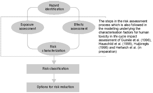
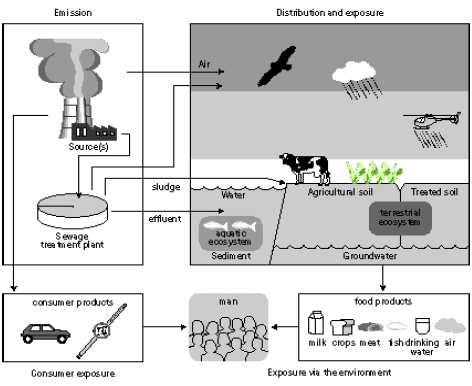
Figure 7.1. Steps in the risk management process (modified from Van Leeuwen and Hermens 1995) Figure 7.1 gives a general scheme for the steps in the risk management as described in the technical guidance documents of the European Commission (EC 1994, 1996). The human toxicity factors of Guinée et al. (1996), Hauschild et al. (1998), Huijbregts (1999) and Hertwich et al (2001) take their basis in those steps encircled in Figure 7.1. First, the increase of environmental exposure or concentration is predicted for one unit of emission of a given substance (exposure assessment), and in parallel the no-effect-concentration or safe dose is predicted (effect assessment). Next, the predicted environmental concentration or exposure (PEC) is divided by the predicted no-effect-level (PNEC) or safe dose. In this way, characterisation factors are obtained following a framework (PEC/PNEC) similar to the one for risk characterisation (PEC/PNEC). The exposure assessment underlying the characterisation factors for use in life cycle assessment calculates similar exposure increases for all releases of the same quantity and substance. Disregarded are the circumstances under which these emissions take place. This contradicts what we intuitively would expect. An example for atmospheric emissions may illustrate this: Exposure increases from an emission released at moderate height will close to the source be considerably higher than those from an elevated release, but lower than those from an emission released at ground level or indoors. The traditional characterisation factors also do not take into account spatial differences in for example atmospheric conditions and population densities between areas. Section 7.2 evaluates the need for spatial differentiation in characterisation factors for human toxicity, and continues by exploring the feasibility of a framework [52] based upon Potting et al. (1999) to establish site-dependent factors that assesses the increases of human exposure from air emissions. The framework takes into account variation in release height, atmospheric conditions, and population densities in the receiving areas. The framework is used to calculate site-dependent factors that quantify the increase of accumulated human exposure from an emission at a given location. Those factors can be used as an exposure factor in combination with the existing characterisation factors for human toxicity from Wenzel et al. (1997). The Guidance Document of Hauschild and Potting (2003) to this Technical Report describes in its entirety how to apply the developed methodology. In contrast to a risk characterisation as described in the technical guidance documents of the European Commission (EC 1994, 1996), the characterisation factors used in life cycle assessment do usually not account for background exposures. They are based on exposure increases rather than actual exposures (sum of the background exposure and the exposure increase). As a consequence, exceedance of the no-effect-levels is not taken into account in these characterisation factors. The predicted exposure increases (PEC) are only weighted with the relevant no-effect-concentration (NEC) for the given substances (PEC/NEC). This weighting is needed to aggregate exposures to different substances. A lively debate is going on whether or not life cycle assessment should perform an evaluation of threshold exceedance. This issue is closer examined in Section 7.3 in which information is also provided for a selection of substances that may facilitate a qualitative threshold evaluation. 7.2 Exposure assessment [53]7.2.1 IntroductionHuman toxicity is a complex impact category. This complexity arises, amongst others, from the numerous possible routes through which an emission can lead to human exposure. Figure 7.2 gives a simplified overview. There are three main routes of human exposure to environmental pollutants: Inhalation of air (part of the exposures via the environment in Figure 7.2), Ingestion of food, water and sometimes even soil (all part of the exposures via the environment in Figure 7.2), and Penetration of the skin after contact with polluted surfaces, air, and sometimes also soil or water (part of consumer exposures in Figure 7.2).
Figure 7.2. Overview of the main routes of human exposure to toxic substances (Van Leeuwen and Hermens 1996). The exposure of humans to environmental pollutants usually takes place via more than one route at the same time (multi-route exposure), but one exposure route is often dominating over the other exposure routes. A typical life cycle assessment focuses on inhalation and ingestion, though skin exposure may be of major relevance within the product system some products (like cloths or cosmetics). Hauschild and Wenzel (1998) provide characterisation factors for over 100 substances to characterise the toxic impact from emissions to air, water and soil. An emission can have a direct effect through exposure to the medium to which it is initially released. However, emissions have often also indirect effects through re-distribution of the substance to another medium than the one to which the substance was initially emitted. The factors of Hauschild and Wenzel (1998) distinguish therefore further between inhalation of air, and ingestion of water and soil. Table 7.1 gives an overview of the resulting nine different characterisation factors, while Annex 7.1, 7.2 and 7.3 list the factors per substance. Hauschild and Wenzel (1998) can be consulted for an extensive description of the backgrounds for these human toxicity factors. Table 7.1: Overview of the characterisation factors provided by Hauschild and Wenzel (1998).
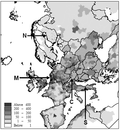
The factors of Hauschild and Wenzel (1998) are based on similar exposure increases for all releases of the same quantity and substance. As clarified in the introduction, this contradicts with what we intuitively expect. Section 7.2.2 evaluates the need for spatial differentiation in the several sub-categories. Section 7.2.3 up to and including Section 7.2.7 explore the feasibility of a framework based upon Potting et al. (1999) to establish site-dependent factors that assess the increases of human exposure from air emissions. 7.2.2 The need for spatial differentiationThe degree to which a source contributes to exposure depends to a large degree on the properties of the substances, the characteristics of the source and the characteristics of the receptor (see also Potting and Hauschild 1997). The characterisation factors of Hauschild and Wenzel (1998) account fully for substance information, but address only to a limited extent information about source and receptor. In addition, Hauschild and Wenzel (1998) do not cover variation in characteristics of sources and receptors. Guinée et al. (1996) allow for some spatial differentiation by distinguishing between exposures resulting from emissions to agricultural soil, industrial soil and to other soils. Huijbregts (1999) continues with this differentiation into soil types, and adds a differentiation into emissions to fresh water and seawater. Differentiation between emissions to different water and soil types may be a useful supplement to the characterisation factors of Hauschild and Wenzel (1998). However, the characterisation factors of both Guinée et al. (1996) and Huijbregts (1999) integrate all types of exposure resulting from emission to the given medium into one characterisation factor. This makes them incompatible to use in combination with the dis-aggregated factors from Hauschild and Wenzel (1998). In the discussions about priority setting for the research underlying Section 7.2, we estimated direct exposures through ingestion of both fresh water and seawater to be small compared to indirect exposures after redistribution (most of the industrialised countries after all purify their water before supplying it as drinking water). Further, we estimated indirect exposure through ingestion of food from agricultural soils by far dominant compared to indirect exposure through ingestion of food from other soils. Differentiation between different water and soil types was therefore not prioritised and is not further addressed in this chapter. Better foundation for refraining from further differentiation in soil and water types is recommended for future research. [54] Distinction between geographic locations of emission is another type of differentiation discussed in priority setting for the research underlying this chapter. We considered this differentiation of major importance for exposures from atmospheric emissions (see Section 7.2.3 up to Section 7.2.7), but of less relevant for exposures from emissions to water and soil. The present state-of-the-art does moreover not allow spatial resolved modelling of direct exposures from emissions to water and soil, and indirect exposures form emissions to all media. Deliberating the importance of the possible and/or relevant spatial differentiation in the several exposure routes, we decided to focus the research underlying Section 7.2 on spatial differentiation in direct human exposure from emissions to air. The results of this research are reported in Section 7.2.3 up to 7.2.7. However, better foundation for refraining from spatial differentiation of exposures from emissions to soil and water is recommended for future research. 7.2.3 Human exposure from air emissions [55]Among the different exposure routes, inhalatory exposures have as a unique feature that they are ubiquitous and can thus not be avoided once a substance is present in air (Williams sine dato). Inhalatory exposures also result in most cases directly from emissions to air rather than being the result of re-distribution between the different environmental media. This chapter focuses only on inhalatory exposures from atmospheric releases. Dispersion and dilution in air are quick processes and the concentration increases at ground level are close to the source very much influenced by wind speeds and source characteristics like height and dynamics of the release (see Figure 7.3). The effective- release height is decisive for the concentration increase at ground level. A moderately high release (25m) has its peak concentration increase within 0.5km from the source, while the peak concentration from a high release (>150m) is a hundred times lower and occurs within 5km. The concentration increase from an emission at ground level (<1m) has its peak within a few metres from the source and is here a thousand times higher than for a similar emission released at a height of 25 metres. Close to the source, the concentration is governed by dilution and the concentration increases are here for all substances almost equal when released at similar release height. The release height becomes less important at increasing distance, however, and removal processes start to take over as is illustrated in Figure 7.4 for the short-lived substance hydrogen chloride and the long-lived substance benzene. Removal processes are largely substance dependent. They are the combined result of deposition and chemical transformations. The emissions of substances with different removal characteristics begin to show their own concentration pattern, and concentration patterns for the emissions of the same substance released at different heights start to converge. At large distances, the height of release becomes negligible and removal processes finally take fully over (see Figure 7.5). Figure 7.3. Concentration increase at ground level versus distance local to the source (from 0 to 5km) from an emission of one gram per second in the Netherlands. Concentration increases have been calculated with the OPS model (Van Jaarsveld 1990, Van Jaarsveld en de Leeuw 1993). The numbers on the y-axis have to be multiplied with the factor for the given release height in the legends to obtain the proper order of magnitude. Figure 7.4. Concentration increase at ground level versus distance semi-local to the source (from 5 to 50km) from an emission of one gram per second in the Netherlands. Concentration increases have been calculated with the OPS model (Van Jaarsveld 1990, Van Jaarsveld en de Leeuw 1993). Figure 7.5. Concentration increase at ground level versus distance local to the source (from 50km to several hundred to thousand kilometres) from an emission of one gram per second in the Netherlands. Concentration increases have been calculated with the OPS model (Van Jaarsveld 1990, Van Jaarsveld en de Leeuw 1993). Atmospheric conditions also influence concentration increases. Wind velocity is of major importance close to the source, whereas precipitation (important for wet deposition) and hours of sunshine (important for photo-chemical transformation) become more important at larger distances. Annual mean atmospheric conditions differ from region to region. Notably wind speeds and precipitation tend to be high in maritime and low in continental climates. The population densities in the area with increased concentrations are the last factor determining the increase of human exposure. Population densities vary considerably over Europe (see Figure 7.6). Western Europe is far more densely populated than North-East and Northern Europe. Neighbouring regions differ less dramatically. Population densities near to the source are of special interest since concentration increases are highest here. Built-up areas show large differences in population densities. (Tobler et al. 1995, Stanners and Bourdeau 1995, EEA1998)
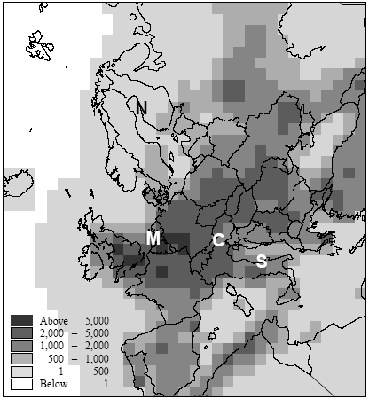
Figure 7.6. Estimate of population densities for 1994 from Tobler et al. (1995). Locations of the Northern, Central, Southern European and maritime sites are indicated with capital letters. Potting et al. (1999) presented a framework to establish site-dependent factors to be used in life cycle assessment that assess the accumulated human exposure increase from outdoor emissions by taking into account all factors described above. This framework could not be applied in its initial form and has therefore been adapted slightly for the research reported here. It consist of 5 steps:
Consecutively, for each source type:
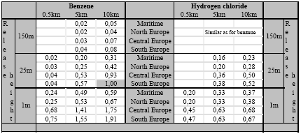
Section 7.2 focuses fully on assessment of exposure increase (Step 1 to 3), but refrains from evaluating whether the exposure situation is above or below a threshold value (step 4). The site-dependent factors that are established in step 5, therefore quantify accumulated exposure increase rather than human toxicity. The site-dependent exposure factors are used in combination with the old characterisation factors in Annex 7.1-7.3 7.2.4 Identification of source types, and classification of processesNear to a source, the release height is decisive for the concentration increases at ground level. The release height for transport will typically be near to ground level (<1m). The information about the release height of industrial processes is usually not available in life-cycle assessment and can vary considerably between sources. The types of industrial processes are on the other hand typically known in life cycle assessment since this is one of its basic informations. An interesting question is therefore whether it is possible to identify source types (or classes of release height) to which industrial processes can be allocated. The Dutch Emission Registration (DER) maintains a rather unique database that contains detailed information about the water and air emissions from over 700 major industrial sources in the Netherlands. Amongst others, the data cover release height, emission type (substance, quantity, flow, temperature), process type and industrial sector. The information is provided mainly by industry itself on a voluntary basis, and to a limited extent also by authoritative bodies like those for water management. All relevant data are recorded for the individual emission points and the individual equipment within each company. (Berdowski et al. 1995) Data from 1994 have been used to analyse whether a relation exists between the height of release points and their connected processes. The median and mean height of release have been determined for records belonging to each industrial sector and for all industrial sectors together. The Statistical Analysis System (SAS Software Release 6.11) was used to analyse the data. The results are presented in Table 7.2. Though these results are expected to give a good indication of release heights, they should only be taken as indicative due to data problems [56] and because they represent data from Dutch industry only. Particularly for countries outside Europe, North America and Japan, the release heights may be considerably lower. Table 7.2: The median, mean and range of release height for each industrial sector in a database containing detailed information about the air emissions from over 700 major industrial sources in the Netherlands based on analyses of data from the Dutch Emission Registration. The overall mean height is 31m with a standard deviation of nearly the same size. However, the median counts only 20 metres due to the majority of individual sectors that have considerably lower means. The mean is pulled up by a few sectors with very high emission points: "Cokes and crude oil refinery/processes", "centralised electricity production & district heating", and "waste processing" (mainly incineration). Excluding these sectors gives a mean [57] height of release for the remaining observations of 25m. The median, mean and range of release height for each industrial sector have been calculated including as well as excluding the own production of energy (steam and/or electricity). The influence of own energy production on the median and mean is for most sectors minor. For a few sectors, the high release heights disappear from the observations without dramatically changing the median and mean when own energy production is excluded. Only the mean height of release for the wood & furniture industry falls considerably (from 20m to 11m). However, we have to take into account the very small number of observations for this sector. The agreement between the mean and the median is for most sectors reasonably good. Also the standard deviations for most sectors are relatively small when the number of observations is reasonable. Most sectors have a relatively low mean height of release: The "extraction of gas, minerals, otherwise" (15m), "textile industry" (17m), "leather preparation" (19m), "wood & furniture industry" (20m), "paper industry " (22m), "printing houses" (15m), "plastic and rubber processing" (15m), metal processing (13m) and the group of "remaining industrial sectors" (17m). The release heights of the percentiles in the higher end are usually also relatively low. Some sectors contain also a few observations of relative high releases, but these observations are in most cases related to own energy production. The "leather preparation" contains only three observations from which two were very low (6 and 7m) and one higher (45m). The "food and tobacco industry" (25m), "chemical industry" (30m) and "glass, pottery, stone and cement industry" (31m) have moderate mean heights of release that are not much influenced by excluding own energy production. The production of sugar, fish flour & glue etc., grass and pulp drying and coffee roasting somewhat pull up the mean height for the "food and tobacco industry". The maximum release height of 100m relates to sugar production. The "chemical industry" contains production of many different chemicals. Most sub-sectors have moderate release heights, but those for the production of inorganic basic chemical and petrochemical products are somewhat higher, while the medians are higher and maximums even very high. The high to very high sources are in most cases related to processes involving some kind of combustion process. The mean release height is relatively high for the "crude oil refinery and processing" (91m), but surprisingly enough rather modest for "electricity production and heating" and "waste processing (mainly incineration)". The mean for "electricity production and heating" increases considerably, however, when the release heights are weighted with the annual production of electricity (133m). Something similar is the case for the "crude oil refinery and processing" and "waste processing". Since these two sectors cover output of several different products, however, it was impossible to calculate a weighted mean. The release heights of "waste processing" are high for processes related to waste incineration (93m). The above results show that the majority of Dutch industry has relatively moderate release heights. This is further underlined by the fact that these results relate to the 700 main industrial sources while the less important ones are not covered. There are only few industries with high sources. The results refer to height of release rather than to "effective release height". The effective release height also includes the plume rise as a result of its heat content. It is actually the effective release height that is relevant for dispersion and dilution calculations. Based on this, three release heights have been chosen for which accumulated exposure increases will be calculated: 1m for traffic, 25m representing the majority of industry, and 150m being a reasonable estimate for high sources. All results here refer to Dutch industry that may not appropriately reflect industry in other countries due to differences in legislation and production capacities and technologies. But the three classes of release heights are expected to be relevant for Europe. 7.2.5 Accumulated human exposure increase local to the source (from 0 to 10km)An atmospheric emission leaves its source in a concentrated form that is sometimes visible as a plume. The plume usually mixes with the surrounding air before it results in concentration increases at ground level. Wind speeds largely determine how fast the plume dilutes, whereas the release height also influences how fast the plume reaches ground level. This is typically modelled with a Gaussian plume approach (Harssema 1995). Atmospheric conditions differ from region to region. Wind speeds tend to be high in maritime and low in continental climates. Van Jaarsveld follows a Gaussian plume approach that applies region-dependent atmospheric conditions (1990 annual statistics mean) in his EUTREND model (Van Jaarsveld 1995, Van Jaarsveld and De Leeuw 1993, Van Jaarsveld et al. 1997). This model is used here to estimate concentration increases at short distances from the source (from 0 to 10km) for different release heights and for sources located in different climates:
The accumulated exposure increase has been calculated for a long-lived substance (benzene; residence time of seven days) and a short-lived substance (hydrogen chloride; residence time of seven hours). These two substances have been selected because the residence time and therewith the accumulated exposure increase from substances will in general be in between those of hydrogen chloride and benzene. The source strength is kept at one gram per second continuous, but the consequence of the release heights as identified in Section 7.2.4 has been analysed (1m, 25m, and 150m). The accumulated human exposure increase from a release on location (i) at each distance is the product of concentration increase times population density integrated over the whole surface: The population density is assumed to be constant (one person·km-2) in the areas local to the source. The result of the calculations is the increase of human exposure (in person·µg·m-3) accumulated over the area from 0 to 10 km from the source. The courses of the accumulated human exposure increase versus distance are depicted in Figures 7.7 to 7.11, and abstracted in Table 7.3. Clear differences exist between the accumulated increase at varying release heights on the one hand, and climate regions on the other hand, as well as between the two substances hydrogen chloride and benzene. Figure 7.7. The increase of accumulated exposure versus distance local to the source (from 0 to 10 km) from one gram benzene released at 1m in four different climatological regions in Europe (population density is one person·km-2). Figure 7.8. The increase of accumulated exposure versus distance local to the source (from 0 to 10 km) from one gram benzene released at 25m in four different climatological regions in Europe (population density is one person·km-2). Figure 7.9. The increase of accumulated exposure versus distance local to the source (from 0 to 10 km) from one gram benzene and hydrogen chloride released at 150m in four different climatological regions in Europe (population density is one person·km-2). Figure 7.10. The increase of accumulated exposure versus distance local to the source (from 0 to 10 km) from one gram hydrogen chloride released at 1m in four different climatological regions in Europe (population density is one person·km-2). Figure 7.11.The increase of accumulated exposure versus distance local to the source (from 0 to 10 km) from one gram hydrogen chloride released at 25m in four different climatological regions in Europe (population density is one person·km-2). Figure 7.11.The increase of accumulated exposure versus distance local to the source (from 0 to 10 km) from one gram hydrogen chloride released at 25m in four different climatological regions in Europe (population density is one person·km-2). Table 7.3. The increase of accumulated exposure from one gram of benzene and hydrogen chloride at different distances from the source (0.5km, 5km and 10km), and released at different heights (1m, 25m and 150m) and in different climate regions in Europe. The accumulated exposures are expressed as the proportion from the accumulated benzene exposure at a height of 25m at 10km distance (20·20km2) in South Europe (69.7 person·µg·m-3). The population density is in all cases one person·km-2.
There is a notable difference in accumulated exposure between the maritime and North European climate regions on the one hand, and the South and Central European climates on the other hand. The climate region becomes more important with lower release heights. This is caused by the considerable difference in wind velocities between the regions. Low wind velocities give slower dilution and subsequently higher concentrations than high wind speeds (direct effect). In addition, low wind velocities go together in a stable and neutral atmosphere with low mixing heights (indirect effect). Decreasing mixing height has an increasing effect on the concentration increase for low sources, but a decreasing effect on the concentration increases for high sources (since they release above mixing height). Wind velocities in the south and central climate regions are on average lower than those are in the maritime and northern climate regions. The direct and indirect effects of wind velocity therefore result in diverging concentrations for low sources, but in converging concentrations for high sources between climate regions. Atmospheric conditions also show variation within regions themselves, as well as over the seasons. However, the subsequent variation in accumulated exposure increase remains within 10% (based on calculations with a similar model that is not further reported here: Van Jaarsveld and De Leeuw 1993). Though benzene and hydrogen chloride have similar accumulated increases at very short distances (< 0.5km), they already show a clear divergence within the first 10km for low release heights. This is mainly due to dry deposition which is considerably higher for hydrogen chloride than for benzene. Emission at 150m will often be above the mixing height and therefore result in increases of accumulated exposures that are nearly the same for both substances. Removal by dry deposition is still very small here since the concentrations at ground levels are small. All accumulated exposures in Table 7.3 and Figure 7.7 to 7.11 relate to a population density of one person·km-2. Tobler et al. (1995) give detailed data about population densities in the European grid. As can be seen from Figure 7.6, which represents this data at regional resolution, population densities vary considerably between European regions (from one to more than five hundred persons km-2). Tobler et al. (1995), EEA (1998) and Stanners and Bourdeau (1995) show that large variation also exists within built-up areas. The population of big cities for instance is distributed rather unequally over the city-area, though generally concentrated in the city-centre. City-centres are mostly limited to an area of at maximum 10 10km (exceptions may be Berlin, London and Moscow). Typical population densities have been defined on the basis of data from Tobler et al. (1995) about Paris:
Hence, the total population of 2.2 million persons in Paris-city (roughly 10 10km2) exceeds by far the total population in most cities and smaller communities. This would even be the case if Paris-city had a population density of 900 person ;km-2 (which would correspond to a total population of 90.000 persons). One thus has to be careful in choosing the population density within the first 10km (or 20 20km2) from the source. While the population density in Figure 7.6 reflects the urbanisation in the relevant region, often no information is available in life cycle assessment about the exact location of a source in relation to built-up areas. We therefore suggest to take the mean population density within the relevant region in Figure 7.6 as the one for those within the first 10km. 7.2.6 Accumulated human exposure increase regional to the source (from 10km to several hundreds to thousand kilometres)At longer distances, the plume from a source in vertical direction is distributed equally in the mixing layer of the atmosphere. Trajectory or one-dimensional Lagrangian modelling is an often-used way to trace concentration increases resulting from substance transport and removal at long ranges (Seinfeld and Pandis 1998). Atmospheric conditions differ from region to region, and notably precipitation and wind speeds tend to be high in maritime and low in continental climates. The Wind rose Model Interpreter (WMI) of the integrated assessment model EcoSense (Krewitt et al. 1997) follows trajectory modelling based on region dependent atmospheric conditions (1990 annual statistics mean). The WMI-module is used here to assess long-range accumulated exposures (see Annex 7.4 for model specifications and adaptations). Similar to the modelling of exposure local to the source, calculations have been performed for hydrogen chloride and for benzene at an emission rate of one gram per second continuous. At the regional scale, release height only has minor importance for a long-lived substance as benzene. However, it will considerably influence the removal by deposition and consequently the amount of a short-lived substance going into long range transport. The calculations for hydrogen chloride have therefore been performed for the release heights 1m, 25m and 150m by correcting for deposition in the source grid-square of respectively 38%, 30%, and 9% of the emissions (see Annex 7.4). Since atmospheric conditions are region-dependent, the patterns of concentration increase will depend on the geographical location of sources. Also population density is region-dependent. The concentration increase in each 150 150km grid-square is multiplied with the total population in that grid-square (derived from the same data as used for Figure 7.6). Next, the products of concentration increase times population in each grid-square are accumulated over the grid (see Formula 7.1). The result is the accumulated exposure increase (in person µg m-3) over a distance of several hundreds to thousands kilometres from a source located in the specified grid-square in the European grid. The procedure is repeated for every grid-square as the source grid-square. The results for hydrogen chloride are represented in Figure 7.12 and the results for benzene in Figure 7.13.
Figure 7.12. The increase of exposure accumulated (in person µg m-3) over the total receiving area (from 10km to several hundred to thousand kilometres) posed by a release of one gram emission hydrogen chloride at 25m in the source grid-square. The mean is 2,460 person µg m-3, the standard deviation is 1600 person µg m-3 (both weighted for population density). The accumulated exposure is attributed to the respective source grid-square. The increase in accumulated exposure from a release at 150m can be obtained by multiplying with a factor 1.30 (s.d. 0.02). The accumulated exposure increase from a release at 1m can be obtained by multiplying with a factor 0.89 (s.d. 0.04).
Figure 7.13. The increase of exposure accumulated (in person µg m-3) over the total receiving area (from 10km to several hundred to thousand kilometres) posed by a release of one gram benzene at 25m in the source grid-square. The mean is 50,000 person µg m-3, and the standard deviation is 33,000 person µg m-3 (both weighted for population density). The exposure increase is extrapolated to transport distances where all benzene is removed from the atmosphere (see Annex). The accumulated exposure is attributed to the respective source grid-square. The patterns of accumulated exposure increase for hydrogen chloride in Figure 7.12 roughly reflect the pattern of population densities in Figure 7.6. The pattern in Figure 7.13 of accumulated exposure increase for benzene is much smoother. Also the variation of exposure increases over the grid is smaller for benzene than for hydrogen chloride. There is a difference of less than a factor 20 for benzene, but almost a factor 100 for hydrogen chloride between highest rating source grid (South-Eastern Netherlands) and the very low rating source grids (in some very sparse populated areas in the far North) of accumulated exposure increase. Accumulated increases are rather close between neighbouring grid-squares. However, the spatial differences are expected to become sharper when exceedance of threshold values would be taken into account (see also Section 7.3). To closer examine the importance of spatial variation in atmospheric conditions and population density, accumulated human exposure increase has been plotted versus distance for seven sites. Four of these sites are similar to the ones selected in Section 7.2.5. The other three sites are the neighbouring grid-squares of the Dutch site. The four Dutch sites experience rather similar atmospheric conditions, but their populations vary considerably (largely explained by the land-water ratio in those grid-squares). The results are represented in Figure 7.14 and 7.15. Figure 7.14. Increase of accumulated exposure for one gram hydrogen chloride released at 25 m at the North, Central, South European and maritime site. To compare dependence of the increase of accumulated exposure increase on climate with dependence on local population, three Dutch sites with similar climate as the maritime site but different population densities have been included. Figure 7.15. Increase of accumulated exposure versus distance for one gram benzene released at 25m at the North, Central, South European and maritime site as a function of distance from the source. To compare dependence of the increase of accumulated human exposure on climate with dependence on local population, three Dutch sites with similar climate as the maritime site but different population densities have been included. Though the residence time of benzene corresponds to a source distance of about 3500km we present model results only up to the distance where the trajectories hit the nearest edge of the model domain. The curves in Figure 7.14 and 7.15 are linearly interpolated due to the accumulated grid-squares each representing a discrete value (being the product of concentration increase and population). The marked sections in the hydrogen chloride diagram illustrate that grid-squares of 150 150km are rather coarse for exposure assessment of a short-lived substance. The model domain as a whole is on the other hand too small to trace a long-lived substance as benzene over its full atmospheric residence time. The residence time of benzene corresponds to a source distance of about 3500km, but the source distance of the nearest edge of the model domain is between 1600km (South and North Europe) and 2400km (Northern Netherlands) for the sites considered here. Due to the longer lifetime, accumulated exposure increase of benzene is less dependent on the population in the source grid-square and more on the regional population than for hydrogen chloride. The curves for the short-lived hydrogen chloride in Figure 7.14 are dominated by the influence of population in the source grid-square (within 80 km from the source), and in the four nearest neighbour grids (step at 150km). The grid-square in the South-Eastern Netherlands extends into Belgium and Germany. It is one of the most densely populated grid-squares with almost 11 million persons. In spite of the high wind speeds that dilute concentrations, the accumulated human exposure increase for emissions in this grid is therefore larger than for the sites in other climate regions. The south-western (maritime) and north-eastern sites in the Netherlands are also densely populated (respectively 6.4 and 4.5 million persons). The next group of curves includes the grid-squares with smaller populations in the North-Western Netherlands and Austria (both 1.5 million persons) and Italy (0.9 million persons). The exposure increase in the North-West Netherlands and Italy source grid squares is almost equal due to high wind speeds in the Netherlands (7 m s-1) that reduce, and low wind speeds in Italy (4 m s-1) that enhance concentration increase. Austria shows a larger exposure increase than Italy, because wind speeds in Austria (5 m s-1) are slightly higher and the population is considerable higher than in Italy. The discussion in the previous section already has shown that atmospheric conditions at the North European site lead to low concentrations. However, in this diagram it is the very low population with 0,2 million persons in the source grid-square and 0.1-0.3 million persons in the adjacent grid-squares that leads to an extraordinarily low human exposure. Accumulated exposure increase of benzene (Figure 7.15) shows to be much less related to the population in the source grid-square but more to regional population than the short-lived hydrogen chloride. Again, the highest accumulated exposure is caused by emissions from the South-Eastern Netherlands. The curve for emissions from the Central Europe grid-square (Austria) is almost catching up though, whereas the population in the source grid-square is by a factor of seven smaller. That is because the Central European site is situated between highly populated areas in the United Kingdom, the Benelux countries, France, Germany, Italy, Hungary, and Poland. The South-Eastern Netherlands has a rather peripheral location on the other hand. Even the South European site is ranking before the North-Western Dutch grid-square. The course of accumulated exposure increase from the four Dutch sites with similar regional populations but different populations in the source grid-square is comparable after several hundred kilometres. Atmospheric conditions have a smaller influence on the pattern of accumulated human exposure increase than expected (not plotted). Even for the short-lived hydrogen chloride, which is rapidly scavenged by precipitation, the wind speed and precipitation show to be of minor importance for human exposure increase accumulated over long distances compared to population. This finding is stronger still for benzene whose small scavenging ratio renders wet deposition negligible and whose atmospheric fate is far less determined by local wind speeds, due to its long transport distances. 7.2.7 Total increase of accumulated exposure from air emissionsTotal exposure increase from an emission is the sum of the accumulated human exposure increase local to the source (from 0 to 10km) and the exposure increase regional to the source (from 10km to several hundreds or thousands kilometres).
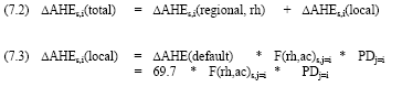
Where: ΔAHEs,i(......) = The factor that relates one gram of substance (s) released at a height (rh) by a source located in grid-square (i), to the increase in accumulated human exposure (in person µg m-3). Local refers to increase within 0 to 10km from the source (20 20km), and regional refers to an increase over a distance of several hundreds to thousands of kilometres from the source. ΔAHE(default) = The factor that relates one gram of substance (s) released at default height (25m) and under default atmospheric circumstances (South Europe), to the increase in accumulated human exposure (in person µg ;m-3) within short distances from the source (<10km) (based on a population density of one person per km2). F(rh,ac)s,j=i = The factor modifying the default increase of accumulated human exposure according to the actual height of release (rh) and the actual atmospheric circumstances (ac) in the receiving area (j=i) local to the source, and the substance released (s) PDj=i = The factor modifying the default increase of accumulated human exposure according to the population density in the receiving area (j=i) The accumulated human exposure increase over long distances from the source can be taken from Figure 7.12 for hydrogen chloride and from Figure 7.13 for benzene. The exposure increase of benzene is hardly influenced by release height and thus for all heights similar. For hydrogen chloride, the data have to be adjusted according to the factors for the relevant release heights that are mentioned in the caption to Figure 7.12. The accumulated human exposure increase local to the source can be calculated from the default of 69.7 person µg m-3 for a population density of one person km-2 multiplied by the population density in the grid-square where the source is located. The default of 69.7 person µg m-3 relates to the exposure increase from benzene and from a release height of 25m in the area of 0 to 10km from the source (20 20km). Table 7.3 provides factors to modify this exposure increase according to the substance being emitted (benzene or hydrogen chloride), the height of release (1m, 25m, 150m), and the climate region in which the source is located. The results of applying Formula 7.2 and 7.3 to an emission of one gram hydrogen chloride and benzene are illustrated in Table 7.4. The table shows basically the same trends as discussed in the previous sections, though the dominance of the accumulated human exposure increase local to the source becomes very strong now for hydrogen chloride. Short-lived substances as hydrogen chloride have a large share of their impact within the first 10km from the source and this is obviously intensified for low heights of release and high population densities. The sensitivity for source height and population density local to the source makes the exposure increase from short-lived substances far more uncertain than the exposure increase from long-lived substances. As Table 7.4 illustrates, long-lived substances as benzene usually will have most of their impact regional to the source. Table 7.4: The sum of the local and regional increase of exposure for one gram of benzene and hydrogen chloride release at 25m at seven sites in Europe.
The analysis of release height for different industrial processes as reported in Section 7.2.4 indicates that a release height of 25m can be taken as default for most processes (the majority of sources have a release height around 25m). It is suggested not to deviate from this default release height of 25m unless a deviating release height is strongly probable. Only release heights for energy production and few other industries (see Table 7.2) typically will be relative high compared to the overall mean. A release height of 1m is relevant for emissions from transport. Population densities will usually be higher in build-up areas (900 person km-2) and city-centres (21,500 person km-2). This will especially have large influence on exposure increase when the source is located in the vicinity of a relatively large city and the peak of the concentration increase occurs in the middle of this city. However, the location of a source in relation to a built-up area will in general not be known in life cycle assessment. In addition, a population density of 900 person km-2 over 10km2 corresponds to a population of 90,000 persons. While a city of that size is as such not unusual, this will often already be reflected in the population density of the region where this city is located (see Figure 7.6). The proposed framework in this chapter therefore suggests taking the population density in the relevant region (see Figure 7.6) to quantify the exposure increase local to the source. The number of toxic substances in a typical life-cycle inventory can be considerable. However, the spatial differentiated exposure factors in this chapter relate to two substances only: Hydrogen chloride and benzene. These two substances have been selected on the basis of their lifetimes. Hydrogen chloride represents substances with a very short lifetime, while benzene represents rather long-lived substances. The exposure increase from other substances will thus in general be in between the increase from hydrogen chloride and benzene. The results for these two substances can therefore with reasonable confidence be used to evaluate spatial variation in source locations. Exposure increase within short distance from the source and over long distances has been quantified with two different models. The models have been calibrated to the extent possible such that input and model data were comparable. Nevertheless, both models are based on different mathematics. The results have been added together without extensively checking how fluently the exposure increase from the local model runs over into the one of the regional model. A rough comparison, which is not further reported here, has been made with results from the OPS-model (Van Jaarsveld 1990, Van Jaarsveld and De Leeuw 1993). This model is limited to source grid-squares in the Netherlands, but fluently integrates modelling of local and regional concentration increases. The comparison suggests that it is reasonable to sum local and regional exposure increases as done here. A better calibration is recommended, however, in combination with quantification of uncertainties related to each model as such and from putting them together. The presented site-dependent factors cover accumulated exposure increase from a release, and disregard whether threshold values are exceeded as a result of the exposure. The spatial differences between the factors are expected to become more pronounced if exceedance of threshold values would be taken into account. 7.3 Effect assessment (evalution of threshold exceedance)7.3.1 IntroductionThe impact assessment phase in life cycle assessment initially emerged from the wish to aggregate the large amount of data from inventory analysis to a manageable amount of impact data. For most impact categories and also for human toxicity, rather simple modelling was used at first to establish characterisation factors. Those characterisation factors were all based on equivalency assessment on the basis of intrinsic substance characteristics. For human toxicity, the emission data from inventory were usually converted in dilution volumes by means of dividing emission data by some kind of threshold value. (Potting et al. 1999, Potting 2000) No assessment of threshold exceedance was performed in this simple modelling since the available data did not allow such evaluation. Threshold information was used in toxicity assessment only to express the emission quantity of a given substance in the volume needed in the amount of receiving environment needed to dilute the emission until the threshold value was reached. The so calculated dilution volumes provided the possibility to aggregate substances with different toxic effects. (Potting et al. 1999, Potting 2000) The basis of equivalency in this simple modelling was taken in the toxicity potential of each substance [58]. The impact from an emission quantity equal to the threshold value was put on one, and the impact from any deviating quantity was assessed as the ratio of that quantity divided by the threshold value for that substance. The underlying assumption was that the toxicity impact from an emission quantity at the threshold value for a substance has the same importance as the toxicity impact from the quantity at the threshold value of another substance. To put it more clearly: If the quantities of both substances are at their threshold value, the impacts from a neuro-toxic substance and an irritating substance are regarded as equally important [59] (Potting et al. 1999). The initial human toxicity factors have later been replaced by factors based on more sophisticated modelling. Present typical toxicity factors as from Guinée et al. (1996), Hauschild and Wenzel (1998), Huijbregts (1999) and Hertwich et al. (2001) now also cover modelling of fate and exposure increase. Aggregation of calculated exposure increases from different substances is still based on threshold values. Where initially occupational standards were often used, however, it is now common practice to use no-effect-concentrations or safe doses. As mentioned in Section 7.2, the presently typical methods for the assessment of human toxicity impact in life cycle assessment do still not take into account background exposures, since they calculate exposure increases rather than actual exposures (sum of background exposure and exposure increase). This section discusses the need for threshold evaluation, and provides information for a selection of substances to implement a qualitative evaluation in life cycle assessment. 7.3.2 Need for evaluation of threshold exceedanceThere is ongoing discussion about whether and how to perform an evaluation of threshold exceedance in life cycle assessment. The discussion is relevant in particular with regard to human toxicity. Human toxicity assessment initially focused on quantifying the probability of surpassing threshold values (like no-effect-concentrations or regulatory standards) in the direct vicinity of emission sources. This focus was directly related to the perceived local character of human toxic impact. Contrary to the present situation, increased pollution levels could in general be traced back to a neighbouring single source (usually large point sources like industry of waste processing). The severity of human toxic and eco-toxic impact local to some sources moved environmental regulation to curb the most pressing situations and prevent similar ones in future. Since then, a large body of policy instruments has been implemented (like licenses, levies and subsidies, and anti-pollution taxes). Risky situations local to sources have in this way been prevented by keeping the emissions from the point source under control. Risk was interpreted as exposure levels above a given threshold. (Potting et al. 1999) Meanwhile, the effective implementation of environmental policies in most of the industrialised countries has led to a situation where the emissions of toxic substances from large point sources in general have been reduced considerably. Large reductions have been achieved by add-on emission reducing technologies or by structural technological improvements in production processes. Risk from a single source to its local environment is nowadays prevented in most cases, and the total emissions from all large point sources together have been reduced substantially for many substances over the last decades. (Potting and Hauschild 1997, Wenzel et al. 1997, Hulskotte et al. 1997, EEA 1998) In spite of the remarkable successes in emission reduction, management of risk from toxic substances is more topical than ever. As mentioned above, individual sources rarely by themselves cause an exceedance of threshold values in their local environment. However, the intricate net of sources and the dispersion of many substances over large distances have led to a widespread presence of a broad variety of different substances that result from many sources together (rather than from a single source). Even though the exposure to an individual substance may remain below its no-effect-concentration, the accumulated exposure to a cocktail of substances may pose a risk. The toxic impact of exposure to a mixture of different substances is unknown, but can be additive or even synergistic. In addition, whereas initially no-effect-concentrations were supposed to exist, there is nowadays growing evidence that a substance may have effects below its assumed no-effect-concentration. This concern is raised by a number of observations of effects on human beings and animals that are highly suspected to relate to such combined exposures. Examples of this are the reduced sperm quality in mens, the increase in testicle cancer and the relative increase in the frequency of female trout in some water bodies (Toppari et al. 1995) and the increase in asthma and allergy among humans in Western European countries. In the present environmental situation, it has become relevant to consider exposure situations both above and below relevant threshold values, but still to evaluate exposures above threshold as being more severe compared to the ones below threshold. This was the main incentive to explore the possibilities for a qualitative evaluation of threshold exceedance in life cycle impact assessment as part of the Danish LCA-methodology development and consensus creation project. 7.3.3 Possibilities for including evaluation of threshold exceedance [60]As demonstrated in Section 7.2.3, the concentration increase from an outdoor source may have a considerable contribution local to that source (from 0 to 10km), but it rapidly becomes smaller at longer distances. Neither close to the source nor at longer distances, however, will outdoor emissions nowadays be expected to cause increases that by themselves lift the ambient concentration from below to above threshold values (see also Section 7.2.3). The ambient concentration at a given location, the concentration that one inhales, is the sum of the existing background concentration and the concentration increase from the given source. Information about the background concentration is thus indispensable to perform an adequate threshold evaluation. The background concentration at a given location is often the result of contributions from more sources together, while these sources can each be close to, or more distant from that location. Obviously, background concentrations in densely populated areas will in general be higher than in sparsely populated areas due to differences in societal and economic activity (i.e., source density). The risk for threshold value exceedance by a concentration increase will therefore also be higher in densely populated areas. At the same time, the accumulated exposure increases are obviously also higher for sources located in densely populated areas (exposure being the product of concentration times population). If exceedance of threshold values had been taken into account, the combined effect of this would probably have resulted in more pronounced spatial differences in the site-dependent factors as established in Section 7.2. Integrated assessment models like the RAINS model described and used in Chapters 3, 4 and 6 are an obvious way to combine the estimation of background concentrations from multiple sources and the concentration increases from an individual source, with population densities and with threshold evaluation. Whereas such models already exist for other impact categories, however, they are only of limited availability for the assessment of human toxicity. Important reasons are the infinite number of potential human toxic substances, their considerable differences in fate, and the differences in number and type of their possible sources. Also for human toxicity assessment, integrated assessment models are expected to become more important. At present, developments take place in that direction for several groups of substances. However, the present state-of-the-art in modelling and data availability regarding toxic substances does not yet allow making such threshold evaluation at more than a qualitative level. One solution is to refrain from inclusion of threshold information in the quantification of human toxicity impact. This assumes that similar exposure increases are equally important, regardless whether the background concentration (together with the concentration increase) is below or above the relevant no-effect-concentration. An intermediate approach could be to consider background concentrations as default being below threshold values, unless they are with high probability close to, or above these values. Such intermediate approach is presented in the next sections. This part of the developed framework also covers indoor situations. 7.3.4 Chosen type of threshold valuesOne threshold figure for exposure, above which effects occur and below which no effects are seen, is a crude simplification of reality. Humans differ in terms of age, size, sex, race and other physiological factors, and consequently they react differently upon chemical exposure. Established "threshold" levels are often based on results obtained from animal experiments at relatively high exposure levels. This implies respectively extrapolation from animal-to-human and from high-to-low dose levels when establishing the threshold levels. In some situations it is further necessary to extrapolate from short-to-long term exposure durations. Threshold levels for the external environment are developed to protect even the more sensitive population groups. Therefore, exposure above the threshold levels will not necessarily result in massive toxicological effects. On the other hand, caution should be taken as definitions of threshold levels for regulatory purposes are sometimes not only based on a toxicological/scientific background but also take on technological feasibility, costs of compliance, prevailing exposure levels, social, economic and cultural conditions (WHO, 1998). WHO stresses that a distinction should be made between WHO guidelines - derived from purely epidemiological/toxicological data - and other "quality standards" (like regulatory thresholds) where the above societal factors may have influenced the levels (WHO, 1998). The same principle is applied by the EU, which operates with both EU Guidelines and EU limit values. The guidelines are based on evaluation of scientific data only and are the levels below which only insignificant effects may be expected, whereas the legally binding limit values may be the result of cost-benefit analyses (EEA, 1997). The developed framework will - where possible – compare actual exposure levels with guidance values; i.e. the guidance values will be considered "threshold". These "threshold levels" include air concentration levels and acceptable/tolerable daily intakes (ADI/TDI's) which are assumed to cause no significant acute and also no chronic effects after life-long exposure/intake. The existence of a threshold - meaning that an exposure level exists below which no toxic effect is seen - is controversial. Some scientists argue that no substances have thresholds, whereas others argue that all substances have. However, the more general assumption is that some substances act via a non-threshold mechanism; especially genotoxic substances. Therefore, acceptable exposure levels for these substances are often expressed as a level, which implies a life long risk of 10-5 or 10-6 of obtaining cancer. 7.3.5 Chosen emission/exposure situations and substancesAs argued in Section 7.3.2, single sources in themselves do usually not evoke exceedance of threshold values for human toxicity anymore. It was after all local problems that initiated the extensive body of process oriented environmental policy. For the purpose of impact assessment in LCA, it seems therefore fair to assume that environmental concentration levels resulting from one single source generally remains below the no-effect-level due to the process oriented policy measures. At least this is expected to be the case for the most developed countries. However, there are exceptions from this assumption. The first exception concerns the zone very closely surrounding the discharge point where exceedance of the no-effect-level may still occur. In environmental regulation, the exceeding of the no-effect-level is accepted within a certain defined dilution zone. This zone is in general situated at, or immediately surrounding the domain of the releasing industry, and might thus be considered a part of the technosphere rather than the ecosphere. It can therefore be argued that LCA can disregard this exception from the marginality assumption in characterisation modelling. (Potting and Hauschild 1997) The second exception concerns occupational exposures and exposures resembling occupational exposures. This type of exposure situations are subject of another part of the Danish LCA-methodology development and consensus creation project. (Schmidt et al. 2000) and not further addressed here. Other human exposure situations, which typically might be near or above thresholds are listed below. The list is a further development of a list prepared at the first workshop of the Danish LCA-methodology development and consensus creation project carried out 15 May 1998.
Inhalation will be the primary exposure route for many of the described exposure situations, but also indirect exposure via drinking water and foodstuffs can be relevant as well as direct skin contact (mainly allergic reactions in the consumer phase). Table 7.5 Overview of situations where guidance values may be exceeded regularly.
¤ To be used with caution. Has been derived from the TDI assuming: 64 kg body weight, inspiration of 22 m³ per day and the same bioavailability/uptake via oral and inhalation exposure. Especially the latter assumption may be questioned. * `bw': Abbreviation for `body weight'. # In relation to LCA, attention must be paid to substances with non-threshold mechanisms, e.g. benzene and particles. For these substances, any elevation in exposure will result in an elevated risk. The recommended threshold levels are therefore less relevant in relation to site characterisation. & For industrialised countries, regulation of point sources will often aim at protecting the surrounding area from above threshold exposure situations. This assumption may often be interpreted as default, but exceptions may occur. It is beyond the scope of this methodology development and consensus project to outline all substance specific exposure situations that may be "near or above threshold". A number of substances have therefore been selected. These substances are those contributing significantly to the EDIP97 normalisation factor for human toxicity (Hauschild and Wenzel, 1998). They are supplemented by a number of other typical and well-known environmental pollutants known as potentially harmful to human health, including particles and some aromatic and/or halogenated substances. The prevailing exposure levels will be outlined and where possible, they will be quantified and compared to threshold levels. An extensive description for each substance is given in Annex 7.6, but the results are summarised in Table 7.5. Background concentrations in the outdoor environment have high probability to be close to or above threshold values on a regional scale in industrialised regions with a highly intricate net of sources emitting the given substance. Maps of regional exposure levels over Europe have been found for mercury (Ryabonshapko et al. 1998), lead and cadmium (Pekar et al. 1998a), lindane, polychlorinated biphenyls and benzo(a)pyrene (Pekar et al. 1998b), photochemical oxidants (Simpson et al. 1997), and nitrogen and sulphur (EMEP/MSC-W 1998). Berdowski et al. (1997) give emission projections over the European grid for a number of persistent organic pollutants and heavy metals. Annex 7.5 gives an overview of addresses where the several reports can be obtained. Annex 7.6 gives a more qualitative description or regional exposure levels together with the exposure levels in those other situations as identified above. It is difficult to give general recommendations on whether or not a specific exposure situation encountered in LCA can be assessed to be near or above "threshold". However, table 7.5 presents a crude summary of the findings of the present paper. The table should not be regarded as bare facts, but as a best attempt to summarise the previous paragraphs, which are again based on the level and extent of the consulted literature. Furthermore, it should be observed that many of the data of the consulted references originate from the beginning of the 1990'ies, since when the situation has been rapidly changing due to for instance new abatement technology and changes in the traffic load. 7.4 ConclusionsThis chapter explores the influence of spatial differences in atmospheric conditions and source characteristics (location, release height, location in relation to built-up area) on the accumulated human exposure increase and subsequent effect from atmospheric emissions. The spatial differences in exposure increase are thoroughly quantified for two substances, the effects of possible exceedance of threshold values are covered in a more qualitative way. Some remarks about the established site-dependent exposure factors and about threshold exceedance have already been made in the previous section. Here, some main conclusions are drawn. There is a difference of less than a factor 20 for benzene, but almost a factor 100 for hydrogen chloride between highest rating (South-Eastern Netherlands) and low ratings (in very sparse populated areas in the far North) of the (regional) accumulated exposure increase. The spatial differences are expected to become sharper when exceedance of threshold values would be taken into account. The population density shows to have the largest influence on the differences in regional exposure increase from sources at different locations. The importance of population density becomes stronger for a short-lived substance like hydrogen chloride that has its increase of exposure predominantly within the first hundred km from the source. Also variation in atmospheric conditions (region-dependent) and source height have an influence on the regional exposure increase. However, their impact is smaller compared to population density. Accumulated exposure increase local to the source is very dominant for short-lived substances as hydrogen chloride. Their impact occurs largely within the first 10km from the source. The sensitivity for source height and population density local to the source makes the (total) exposure increase from these substances far more uncertain than the exposure increase from long-lived substances that have most of their impact regional to the source. The majority of industrial sources appear to have a release height around 25m and it is therefore suggested to take this as default unless a deviating release height is strongly probable. Only release heights for energy production and few other industries will typically be higher (see Table 7.2), and those for transport will be typically lower compared to the overall mean. It is suggested to take the population density in the relevant region (see Figure 5.4) to quantify the exposure increase local to the source (from 0 to 10km). Population densities will usually be higher in build-up areas (900 person km-2) and city-centres (21000 person km-2). However, the location of a source in relation to built-up area is in general not known in LCA. The number of toxic substances in a typical life cycle inventory can be considerable, while the spatially differentiated exposure factors in this chapter relate to two substances only. The exposure increase from other substances will thus in general be in between the increase from hydrogen chloride and benzene. These two substances can therefore with reasonable confidence be used to evaluate the effect on accumulated human exposure increase from spatial variation in source locations. It is difficult to give general recommendations on whether or not a specific exposure situation encountered in LCA can be assessed to be near or above "threshold". Table 7.5 presents a crude summary of the findings of the present paper, however, that can be used for a qualitative evaluation of possible exceedance of threshold values. This chapter does unfortunately not result in a set of factors integrating exposure and subsequent effect (from threshold exceedance), that can be used to characterise the contributions of various substances and emission situations to human toxicity in life cycle assessment. The state-of-the-art in modelling human toxicity does not allow such integrated factors, however. The material produced in this chapter can merely be used for sensitivity analysis in life cycle assessment. Hauschild and Potting (2003) describe in detail how this can be done. The work in this chapter focuses on direct exposure and effect from atmospheric emissions. Spatial differences with regard to other exposure routes were regarded less important and not addressed (see Section 7.2.2). Huijbregts et al. (2003) assessed in a recent study the effect of using different generic environmental conditions (typical conditions in Australia, Western Europe, and the United States of America). It was found that the uncertainty in fate and exposure factors for ecosystems and humans due to choices of different sets of environmental conditions is between a factor 2 and 10. Particularly, fate and exposure factors of emissions causing effects in fresh water ecosystems and effects on human health have relatively high uncertainty. This uncertainty is mainly caused by the continental difference in the average soil erosion rate, the dimensions of the fresh water and agricultural soil compartment, and the fraction of drinking water coming from ground water. These results encourage to closer look into spatial issues of these exposure routes as well. 7.4.1 AcknowledgementThe authors like to express their gratitude to Burkhard Wickert (IER, University of Stuttgart) for processing of the population data on the Geographical Information System. The work for this chapter was also supported by a Training & Mobility grant from the European Commission, by means of the European Commission under the JOULE Program, and under the EUREKA project LCAGAPS by means of the Danish Agency for Industry and Trade. 7.5 ReferencesATSDR (1997a). Toxicological Profile for Benzene (Update). Agency for Toxic Substances and Disease Registry, Public Health Service, U.S. Department of Health and Human Services. ATSDR (1997b). Toxicological Profile for Chlorinated dibenzo-p-dioxins. (Draft for Public comment). Agency for Toxic Substances and Disease Registry, Public Health Service, U.S. Department of Health and Human Services. ATSDR (1997c). Toxicological Profile for Lead (Draft for Public comment). Agency for Toxic Substances and Disease Registry, Public Health Service, U.S. Department of Health and Human Services. ATSDR (1997d). Toxicological Profile for Cadmium (Draft for Public comment). Agency for Toxic Substances and Disease Registry, Public Health Service, U.S. Department of Health and Human Services. ATSDR (1997e) Toxicological Profile for Mercury (Draft for Public comment). Agency for Toxic Substances and Disease Registry, Public Health Service, U.S. Department of Health and Human Services. ATSDR (1998). Toxicological Profile for Sulfur dioxide (Draft for Public comment). Agency for Toxic Substances and Disease Registry, Public Health Service, U.S. Department of Health and Human Services. Berdowski, J.J.M., W.J. Jonker, P. Verhoeve. Emissions in the Netherlands. Industrial sectors and regions in 1993 and estimates for 1994. No. 27 in publication series emission registration (In Dutch). The Hague (the Netherlands), Dutch Ministry of Housing, Spatial planning and the Environment, 1995. Berdowski, J.J.M., J. Baas, JP.J. Bloos, A.J.H. Visschedijk and P.Y.J. Zandveld. The European Atmospheric Emission Inventory of Heavy Metals and Persistent Organic Compounds. Forchungsbericht 104 02 672/03. Umweltbundesamtes and TNO Institute of Environmental Sciences, Energy Research and Process Innovation, 1997. Berge, E. Six-hourly data in the EMEP 150 km grid. Written communication and data on magnetic tape. Oslo (Norway), EMEP Meteorological Synthesising Centre – West, 1994. Derwent, R.G., and K. Nodop. Long-range transport and deposition of acidic nitrogen species in north-west Europe. Nature, Vol. 324 (1986), November Issue, pp. 356-358, 1986 EC. Risk assessment of existing substances. Technical guidance document in support of the commission regulation (EC) no. 1488/94 on risk assessment for existing substances in accordance with council regulation (EEC) no. 793/93 (XI/919/94-EN). Brussels (Belgium), Directorate General Environment, Nuclear Safety and Civil Protection from the European Commission, 1994. EC. Technical guidance document in support of the commission directive 93/67/EEC on risk assessment for new notified substances and the commission regulation (EC) no. 1488/94 on risk assessment for existing substances. Ispra (Italy), European Bureau of Chemicals, 1996. EEA. Europe's environment. Statistical compendium for the second assessment. Copenhagen (Denmark), European Environment Agency, 1998. EEA (1997). European Environmental Agency. Air pollution in Europe 1997. EEA Environmental Monograph No. 4. Copenhagen. ISBN 92-9167-059-6. ETCAE (1997). Corinair 94. Summary report. Final Version. Report to the European Environment Agency from the European Topic Centre on Air Emissions. European Council (1998). Common position (EU) No. 40/98 outlined by the council 16 June 1998 regarding limitation of the emission of volatile organic compounds from the application of organic solvent in certain activities and facilities. Guinée, J., R. Heijungs, L. van Oers, D. van de Meent, T. Vermeire and M. Rikken. LCA impact assessment of toxic releases. Generic modelling of fate, exposure and effect for ecosystems and human beings with data for about 100 chemicals (series of publication concerning product policy, no. 1996/21). The Hague (the Netherlands), Dutch Ministry of Housing, Spatial planning and the Environment, 1996. Harssema, H. Calculating and measuring air quality (H100-204). Wageningen (the Netherlands), Wageningen Agricultural University, 1995. Hauschild, M.Z. and H. Wenzel: Environmental assessment of products. Vol. 2 - Scientific background, 565 pp. Chapman & Hall, United Kingdom, 1998, Kluwer Academic Publishers, Hingham, MA. USA. ISBN 0412 80810 2 Hauschild, M. and J. Potting. Spatial differentiation in life cycle impact assessment – the EDIP2003 methodology. Guideline from the Danish Environmental Protection Agency, Copenhagen, 2003. Hertwich E.G., S.F. Mateles, W.S. Pease, T.E. McKone. Human toxicity potentials for life-cycle assessment and toxics release inventory risk screening. Environmental Toxicology and Chemistry, 20:928-939, 2001. Huijbregts, M.A.J. Priority assessment of toxic substances in the frame of LCA. Development and application of the multi-media fate, exposure and effect model USES-LCA. Amsterdam (the Netherlands), Interfaculty dept. of Environmental Science, 1999. Huijbregts, M.A.J., S. Lundi, T.E. McKone and D. van de Meent. Geographical scenario uncertainty in generic fate and exposure factors of toxic pollutants for life-cycle impact assessment. Chemosphere, Vol. 51, issue 6, pp. 501–508. Hulskotte, J.H.J., G.P.J. Draaijers, J.J.M. Berdowski, W.L.M. Smeets and C.S.M. Olsthoorn. Recalculations of emissions to air for the period 1990-1996 (in Dutch). Publication series Emission Registration no. 41. The Hague (the Netherlands), Dutch Ministry of Housing, Spatial planning and the Environment, 1997. Jensen B, Wolkoff P (1996). VOCBASE - odour and mocous membrane irritation thresholds and other physico-chemical properties. 2.1. National Institute of Occupational Health, Copenhagen. Jensen B, Wolkoff P (1997). VOCBASE – a database of odour thresholds, irritation of mucous membranes and chemical parameters for volatile organic compounds (in Danish). Dansk Kemi; 5: 16-17, 20-26. Krewitt, W., P. Mayerhofer, R. Friedrich, A. Trukenmüller, T. Heck, A. Greßmann, F. Raptis, F. Kaspar, J. Sachau, K. Rennings, J. Diekmann, B. Praetorius. ExternE – Externalities of energy. National implementation in Germany (EUR 18271). Directorate-General XII for Science, Research and Development of the European Commission, 1997. Krüger, O., J.P. Tuovinen. The effect of variable sub-grid deposition factors on the results of the Lagrangian long-range transport model of EMEP. Atmospheric Environment, Vol. 31 (1997), Issue 24, pp.4199-4209. Metcalfe, S.E., J.D. Whyatt, R.G. Derwent. A comparison of model and observed network estimates of sulphur deposition across Great Britain for 1990 and its likely source attribution. Quarterly Journal of the Royal Meteorological Society, Vol. 121 (1995), Issue 526 (July), Part B, pp.1387-1411. NYSDEC (1995). Ambient air monitoring report for volatile organic compounds. Division of air resources - Bureau of Air Quality Surveillance. Summary of Toxic Monitoring Data from 1990 to 1993. New York State Department of Environmental Conservation. Reports can be obtained from: Bureau Director - BAQS, 50 Wolf Road, Albany, NY 12233-3256. Information in this paper has been retrieved from the Internet: http://www.dec.ny.us/website/pollution/voc_rpt.html. Potting J, Hauschild M (1997). Predicted environmental impact and expected occurrence of actual environmental impact. Part II: Spatial differentiation in life-cycle assessment via the site-dependent characterisation of environmental impact from emissions. Int. J. LCA, 4: 209-16. Potting, J., M. Hauschild, and H. Wenzel. "Less is better"and "only above threshold"; Two incompatible paradigms for human toxicity in life-cycle assessment? International Journal of Life Cycle Assessment, Vol. 4 (1999), Issue 1, pp.16-24. Potting, J. A. Trukenmüller, H. van Jaarsveld and M. Hauschild. Human exposure from air emissions. In: Potting, J. Spatial differentiation in life cycle impact assessment. Ph.D. thesis. Utrecht (the Netherlands), 2000. Potting, J. Spatial differentiation in life cycle impact assessment. Ph.D. thesis. Utrecht (the Netherlands), 2000. Schmidt, A., Rasmussen, P. B., Andreasen, J., Fløe, T. and K. E. Poulsen. Integration of the working environmennt in life cycle assessments (LCA) – a new methodology. Guidelines from the Danish Environmental Protection Agency No. xxx 2000, Copenhagen (2000) Seinfeld, J.H. and S.N. Pandis. Atmospheric chemistry and physics: From air pollution to climate change. New York (United States of America), John Wiley & Sons, 1998. Stanners, D. and P. Bourdeau. Europe's environment. The dobris assessment. Copenhagen (Denmark), European Environment Agency, 1995. Tobler, W., U. Deichmann, J. Gottsegen and K. Maloy. The Global Demography Project (technical Report TR-95-6 [online]). Santa Barbara (United States of America), dept. of Geography, University of California of the National Centre for Geographic Information and Analysis, 1995 [cited 11 August 1999]. Available from Internet http://www.ciesin.org/datasets/gpw/globldem.doc.html. Toppari, J., J.C.Larsen, P. Christiansen, A. Giwercman, P. Grandjean, L.J. Guillette, B. Jégou, T.K. Jensen, P. Jouannet, N. Keiding, H. Leffers, J.A. McLachlan, O. Meyer, J. Müller, E. Rajpert-DeMeyts, T. Scheike, R. Shapre, J. Sumpter and N.E. Skakkebæk. Male reproductive health and environmental chemicals with estrogenic effects (Miljøprojekt no. 290). Danish Environmental Protection Agency, Copenhagen, 1995. Trukenmüller, A. Using WMI: Implementing atmospheric trajectory models with the Wind rose Model Interpreter. Stuttgart (Germany), IER of the University of Stuttgart, 1998. van der Ven B (1995). Default values. A discussion paper for the meeting of the SETAC workgroup "Data handling" on Sep. 4th 1995 at Gothenborg. Van Jaarsveld, H. An operational atmospheric transport model for priority substances; specification and instructions for use. Report number 222501002. Bilthoven (the Netherlands), RIVM, 1990. Van Jaarsveld, J.A. Modelling the long-term atmospheric behaviour of pollutants on various spatial scales. Utrecht (the Netherlands), PhD thesis, Utrecht University, 1995. Van Jaarsveld J. A., W. A. J. van Pul and F. A. A. M de Leeuw. Modelling transport and deposition of persistent organic pollutants in the European region. Atmospheric Environment Vol. 1997, Issue 31, pp. 1011-1024 Van Jaarsveld, J.A. and F.A.A.M de Leeuw. OPS: An operational atmospheric transport model for priority substances. Environmental Software, Vol. 1993, Issue 8, pp. 91-100. Van Leeuwen and J.L.M. Hermens. Risk assessment of chemicals: An introduction (ISBN 0-7923-3740-9). Dordrecht (the Netherlands), Kluwer Academic Publishers, 1995/1996. Wenzel, H., Hauschild M.Z. and Alting, L.: Environmental assessment of products. Vol. 1 - Methodology, tools, techniques and case studies, 544 pp. Chapman & Hall, United Kingdom, ISBN 0 412 80800 5, Kluwer Academic Publishers, Hingham, MA. USA., 1997. Wolkoff P, Clausen P A, Nielsen G D (1998). Volatile organic compounds (VOCS) in the indoor environment. State-of-the-science report. AMI Dokumentation 2. Arbejdsmiljøinstituttet, Copenhagen. In Danish. Wolkoff P, Nielsen P A (1993). Statens Byggeforskningsinstitut. Indeklimamærkning af byggevarer. Del 2: Faglig og teknisk dokumentation af en prototypeordning. SBI-rapport 233. Statens Byggeforskningsinstitut. In Danish. WHO/UNEP (1992). Urban air pollution in Megacities of the World. World Health Organisation, United Nation Environment Programme, Blackwell, Oxford. WHO (1992). Environmental Health Criteria 134. Cadmium. International Programme on Chemical Safety (IPCS), World Health Organisation, Geneva. WHO (1993). Environmental Health Criteria 150. Benzene. International Programme on Chemical Safety (IPCS), World Health Organisation, Geneva. WHO (1994a). Environmental Health Criteria 163. Chloroform. International Programme on Chemical Safety (IPCS), World Health Organisation, Geneva. WHO (1994b). Environmental Health Criteria 170. Assessing human health risks of chemicals: Derivation of guidance values for health-based exposure limits. International Programme on Chemical Safety (IPCS), World Health Organisation, Geneva. WHO (1995). Environmental Health Criteria 165. Lead. International Programme on Chemical Safety (IPCS), World Health Organisation, Geneva. WHO (1997a). Environmental Health Criteria 188. Nitrogen Oxides (second edition). International programme on chemical safety (IPCS), World Health Organisation, Geneva. WHO (1997b). Environmental Health Criteria 195. Hexachlorbenzene. International Programme on Chemical Safety (IPCS), World Health Organisation, Geneva. WHO (1998). Air Quality Guidelines for Europe, World Health Organisation, Regional Office for Europe, Copenhagen, WHO Regional Publications, European Series. (NB! Information for this paper has been retrieved via the Internet addresses: http://www.who.dk and http://www.who.org/peh/specprg.htm.) Williams, M. (ed.). Exposure assessment. Report number 1. Cost 613/2 Report series on air pollution epidemiology. Directorate-General XII for Science, Research and Development of the Commission of the European Communities. Annex 7.1 Characterisation factors for human toxicity assessment from emissions to air
Annex 7.2 Characterisation factors for human toxicity assessment from emissions to water
Annex 7.3 Characterisation factors for human toxicity assessment from emissions to soil
Annex 7.4 Specifications for the Wind rose Model InterpreterDerwent and Nodop (1986) introduced a climatological concept to trace concentration increases resulting from substance transport and removal in the long range. This concept has been used since then in several acid deposition models (e.g. Metcalfe et al. 1995). This concept is also the basis of the Wind rose Model Interpreter (WMI) of the EcoSense integrated assessment model (Krewitt et al. 1997). The modelling approach is receptor oriented and differentiates between twenty-four sectors of the wind rose, such that from each sector a straight-line trajectory arrives at the receptor point. Concentrations at that point are obtained by averaging over the results from these trajectories, suitably weighted by the frequencies of winds in each 15º sector. WMI provides a chemical kinetics interpreter that supports stationary trajectory modelling with arbitrary mass balance and following straight lines on a variety of model grids (Trukenmüller 1998). For the present study WMI has been employed to set up a single layer model with a horizontal resolution of 150 150 km2 on the EMEP [63] grid. Input data of our model have been taken from the EcoSense data-base and include 1990 annual amounts of precipitation and 945 hPa wind roses at each grid-square. These data are aggregated values of six-hourly output of the LAM50E (Limited Area Model, 50 km, Europe) numerical weather prediction model at the Norwegian Meteorological Institute (Berge 1994). Our model uses a constant mean mixing height, which is derived from meteorological statistics for long-distant transport. Those statistics, and parameterisation of removal by dry and wet deposition and chemical conversion of hydrogen chloride and benzene have been taken from Van Jaarsveld (1990): Table A: Parameter-values used to model dry and wet deposition, chemical conversion and vertical mixing in the single layer trajectory model employed for the assessment of regional accumulated human exposure.
The assumption of instantaneous vertical mixing in the single layer model leads to an underestimation of near surface concentrations at distances less than some 10 km from the source. The underestimation of near source concentrations has no direct influence on the assessment of this local human exposure in this study where we use EUTREND results at short distances. However, it entails an underestimation of dry deposition in the source grid-square and therewith an overestimation of the transport to other grid-squares and thus accumulated exposure (Krüger and Tuovinen 1997). The `local dry deposition' has significant influence on the mass balance for hydrogen chloride. We have evaluated local deposition of hydrogen chloride by comparing dry deposition of the trajectory model in the source grid-square with deposition estimates obtained from the Gaussian OPS model (Van Jaarsveld 1990) for the various release heights. Based on this comparison, release height and wind speed dependent local deposition factors have been derived, assuming that a corresponding fraction of emissions is deposited directly to the source grid-square. High wind speeds dilute concentrations and thus decrease human exposure close to the source, but increase the distances over which a substance is transported. Transport over larger distance results in more people being exposed to the (albeit lower) concentration. The direct net effect of high wind speed on accumulated exposure is therefore usually small. There are also indirect effects of wind speed, which tend to decrease concentration and thus accumulated exposure. Wind speed influences mixing height (as discussed in the section 7.2.5), as well as the aerodynamic resistance and the pseudo-laminar layer resistance, which are relevant for removal by dry deposition. These indirect effects, unlike the direct ones, do not cancel out each other, but they are small (second order) and not taken into account in the simple trajectory model here. Dutch mixing height and dry deposition statistics from Van Jaarsveld (1990) are assumed valid for the whole of Europe. Spatial variability of precipitation is considered in the trajectory model here. While wet deposition is of minor importance for benzene, hydrogen chloride is removed from the atmosphere with every shower due to its great scavenging ratio (see Table A). Mean annual removal rates by wet deposition in the Netherlands have been derived for both substances from the empirical relation and statistics of probability, amount and duration of rainfall presented in Van Jaarsveld (1990). Those Dutch removal rates are extrapolated to the whole model domain by linear scaling with the amount of annual precipitation in each grid-square. The implicit assumption behind this scaling exercise is that the number of precipitation events per year is proportional to the amount of annual precipitation, or that the long-term mean of rainfall amount per shower is approximately the same in each grid-square. Precipitation varies largely over the grid. Annual rainfall amounts to 2000–3200 mm a-1 in grid-squares at the Norwegian coast around Bergen. Between 1500-2000 mm a-1 are found at the Western Irish and Scottish coast, in North-West Spain and some alpine grid-squares in Switzerland and Austria. However, precipitation is less than 200 mm a-1 in the Sahara Desert, parts of Turkey, South-East Russia and Kazakhstan. As a consequence, the assessment of annual wet deposition equals that of dry deposition of hydrogen chloride in the Bergen grid-square, while wet deposition is negligible in the low precipitation regions. The calculated minimum atmospheric residence time of hydrogen chloride is 4.4 h for emissions in the Bergen grid, while the maximum is 8.5 h in the Sahara Desert and Kazakhstan. For 80% of the model domain the residence time is almost constant at 6.9 h with a standard deviation of only 14%. These numbers apply to high sources (150 m) and do not include the increased dry deposition (and thereby further reduced importance of wet deposition) local to the source from low releases. Thus, even though precipitation varies largely, its impact on lifetime and accumulated exposure shows little variation and that is therefore not visible in Figure 7.13, because the grey scale in that map only resolves differences greater than a factor 2. Due to the longer lifetime of benzene, accumulated exposure to that substance is less dependent on local and more on regional population density. The model domain is too small to trace benzene concentrations over their full residence time. Approximately 40% of the benzene emitted at the Central European site and almost 60% of the benzene emitted at the North European site is subject to atmospheric transport beyond the edges of the model grid. Those figures have been calculated from the difference of the emitted and the removed substance in the WMI report concerning removal by both deposition and chemical conversion. Similar mass balances have been derived for emissions from each grid-square and used to extrapolate accumulated exposure until all emitted substance is removed. This extrapolation roughly doubles the `raw' exposure assessment of the model. It gives an overestimate by assuming European population density also for the adjacent areas of the Atlantic, the polar sea, Siberia, and the Sahara Desert. So the actual accumulated exposure is expected to be in the range of 50–100% of Figure 7.13, provided model estimates within the grid are accurate. Annex 7.5 Addresses of reports about regional emissions and exposuresFurther information on regional emissions, deposition patterns and/or background concentrations for several of the substances treated may be found in the following literature/references: "Transboundary acidifying air pollution in Europe. Part 1: Estimated dispersion of acidifying and eutrophying compounds and comparison with observations". EMEP/MSC-W. Report 1/98. July 1998. "Transboundary acidifying air pollution in Europe. Part 2: Numerical Addendum". EMEP/MSC-W. Report 1/98. July 1998. "Photochemical oxidant modelling in Europe: multi-annual modelling and source-receptor relationships." EMEP/MSC-W. Report 3/97. July 1997. "Atmospheric supply of nitrogen, lead, cadmium, mercury and lindane to the Baltic Sea." EMEP/MSC-W. Note 3/98. July 1998. "Long-range transport of selected persistent organic pollutants" Part I (EMEP/MSC-E 2/98) "Mercury in the atmosphere of Europe: concentrations, deposition patterns, transboundary fluxes" (EMEP/MSC-E 7/98) "Modelling of long-range transport of lead and cadmium from European sources in 1996." (EMEP/MSC-E 5/98) Berdowski, J J M et. al (1997). "The European atmospheric emission inventory of heavy metals and persistent organic pollutants for 1990". Forshungsbericht 104 02 672/03. EEA (1997), se general reference list. ftp://info.rivm.nl/pub/lae/edgarv20/ For future information retrieval on background levels, the following contacts are valuable: EMEP Meteorological Synthesizing Centres West (MSC-W) Det norske meteorologiske institutt (DNMI) EMEP Meteorological Synthesizing Centres East (MSC-E) Sergey Dutchak Meteorological Synthesizing Centre- East Keldrova U1. 8-1 117 321 Moscow (msce@sovam.com) TNO - Department for Ecological Risk Studies 7.6 Annex 7.6 Exposure situations "near or above threshold"Author: Frans Møller Christensen 1 Introduction The aim of this annex paper is to describe typical "near to, or above threshold human exposure situations" in terms of typical/rule-of thumb magnitude and duration, as an input to the development of a site factor framework for assessment of human toxicity in LCA. Exposure situations covered by this annex paper: Human exposure in or via the external environment (mainly inhalation of ambient air and intake of foodstuffs and water) Indoor exposure (excluded are occupational exposure, and exposure situations resembling occupational exposure, for instance painting) Consumer exposure (excluded are exposure situations resembling occupational exposure, for instance painting) 2 Threshold One threshold figure for exposure, above which effects occur and below which no effects are seen, is a crude simplification of reality. Humans differ in terms of age, size, sex, race and other physiological factors, and consequently they react differently upon chemical exposure. Further, established "threshold" levels are often based on results obtained from animal experiments at relatively high exposure levels, which implies respectively extrapolation from animal-to-human and from high-to-low dose levels when establishing the threshold levels. In some situations it is further necessary to extrapolate from short-to-long term exposure periods. Threshold levels for the external environment are developed to protect even the more sensitive population groups. Therefore, exposure above the threshold levels will not necessarily result in massive toxicological effects. On the other hand, caution should be taken as definitions of threshold levels for regulatory purposes are sometimes not only based on a toxicological/scientific background but also take on technological feasibility, costs of compliance, prevailing exposure levels, social, economic and cultural conditions (WHO, 1998). WHO stresses that a distinction should be made between WHO guidelines - derived from purely epidemiological/toxicological data - and other "quality standards" (like regulatory thresholds) where the above societal factors may have influenced the levels (WHO, 1998). The same principle is applied by the EU, which operates with both EU Guidelines and EU limit values. The guidelines are based on evaluation of scientific data only and are the levels below which only insignificant effects may be expected, whereas the legally binding limit values may be the result of cost-benefit analyses (EEA, 1997). Throughout this paper, actual exposure levels will - where possible - be compared with guidance values; i.e. the guidance values will be considered "threshold". These "threshold levels" include air concentration levels and acceptable/tolerable daily intakes (ADI/TDI's) which are assumed to cause neither significant acute nor chronic effects after life-long exposure/intake. The existence of a threshold - meaning that an exposure level exists below which no toxic effect is seen - is controversial. Some scientists argue that no substances have thresholds, whereas others argue that all substances have. However, the more general assumption is that some substances act via a non-threshold mechanism; especially genotoxic substances. Therefore, acceptable exposure levels for these substances are often expressed as a level, which implies a life long risk of 10-5 or 10-6 of obtaining cancer. 3 Typical high concentration exposure situations Human exposure (except occupational) situations, which are believed to be typically near or above thresholds are listed below. The list is a further development of a list prepared at the first workshop in sub-project V of the LCA-methodology project carried out 15 May 1998. Urban areas, especially with high traffic intensity [64] Long range transport of some air pollutants which may elevate regional background concentrations considerably Areas around point sources [65] Accidents (accidental risk is usually considered separately in LCA) Indoors Direct consumer exposure to products; for instance cosmetics (containing heavy metals, preservatives, perfumes and oxidised tensides which may all cause allergic reactions), textiles (containing for instance azo dyes, some of which may provoke allergic reactions), toys (which have appeared to contain potentially carcinogenic and endocrine acting substances) and a variety of products containing chromium and/or nickel (both being allergens) Inhalation will be the primary exposure route for many of the described exposure situations, but also indirect exposure via drinking water and foodstuffs can be relevant as well as direct skin contact (mainly allergic reactions in the consumer phase). 4 Typical substances involved in high exposure situations It is beyond the scope of this paper to outline all substance specific exposure situations which may be "near or above threshold". A number of substances have been selected for a narrower study. The substances selected are those contributing significantly to the 1990 EDIP normalisation factor for human toxicity (Hauschild and Wenzel, 1998). They are supplied with a number of other typical and well-known environmental pollutants known as potentially harmful to human health, including particles and some aromatic and/or halogenated substances. The prevailing exposure levels will be outlined and where possible, they will be quantified and compared to threshold levels. References in this paragraph will mainly be WHO/IPCS (World Health Organisation/ International Programme on Chemical Safety) and ATSDR (Agency for Toxic Substances and Disease Registry) criteria documents. Further information and original references can be found in these documents. 4.1 NO2/NOx NOx covers both NO and NO2 with NO2 being the more toxic. Often just NOx is measured and/or given in tables. In the present EDIP methodology, NOx is considered to be NO2. This assumption is also used here and is partly justified by the fact that NO often will be oxidised to NO2 by ozone (EEA, 1997). The main outdoor NOx sources are combustion processes. According to Corinair94 (ETCAE, 1997), about 50% of the European emission comes from "Road transport" [66] , a little less than 20% from "Combustion in energy and transformation industry" and 10-15% from "Other mobile sources and machinery". The mobile source contribution to NOx emission is estimated to be between 20 and 80% in different megacities of the world (WHO/UNEO, 1992; see also WHO, 1997a). Indoor NOx-sources comprise gas stoves, unvented (i.e. unventilated) gas space heaters and water heaters, Kerosene space heaters, wood stoves and tobacco products (WHO, 1997a). WHO (1997a, 1998) suggests the following health-based guidance values for NO2: Short term: 200 µg/m³ (0.11 ppm) as a one-hour average daily maximum. Long term: 40 µg/m³ (0.023 ppm) as an annual average. EEA (1997) cites another WHO guidance value of 150 µg/m³ (0.086 ppm) as a 24-hour average. Average annual concentrations in large American, European and Asian cities often exceed 40 µg/m³ (WHO, 1997a). In Europe it is estimated that about 40% of the urban population (27 mio. individuals) is exposed to an annual average above 50 µg/m³ (EEA, 1997). In many major cities one-hour average exposure levels of above 400 µg/m³ occur regularly (WHO, 1997a). Maximum 24-hour concentrations regionally may reach 60-70 µg/m³ in most of central Europe (EEA, 1997). These exposure levels are well below the indicated WHO 24-hour guidance value and as such judged not to pose a health risk to the population outside urban areas (EEA, 1997). Indoor NOx-concentrations rely on a number of factors including outdoor concentration, ventilation rates and indoor sources. In homes without indoor sources, the NOx-level has been measured to 26-80% of the outdoor level (WHO, 1997a). Thus indoor concentrations even in homes without indoor sources may in some situations exceed the WHO annual average guidance value of 40 µg/m³. In about 45% of American homes and up to 100% in some other countries, gas is used for cooking, heating water or drying clothes. Indoor NO2-concentrations in excess of 100 µg/m³ (average over one-two weeks) have been measured. Data on indoor short term concentrations, suggest levels several times higher than the average values, i.e. situations with short term concentrations above 200 ?g/m³ may frequently occur. Concentrations are higher during the wintertime with high heat production and reduced ventilation, and concentration gradients usually exist from the indoor point source to other parts of the home (WHO, 1997a). Indoor NO2-concentrations may be even higher in homes with unvented gas space heaters and Kerosene heaters. One study indicates NO2-concentrations of 100 µg/m³ (average over one-two weeks) for 50% and above 480 µg/m³ for 8%, respectively, in homes with Kerosene heaters. A peak value of 847 µg/m³ was measured. A large field study showed concentrations above 100 µg/m³ in 70% and above 480 µg/m³ in 20% of homes with unvented gas space heaters (WHO, 1997a). 4.2 SO2 The major source of SO2 in the environment is fuel combustion in connection with energy & transformation industries as well as manufacturing industries. These sources contribute to 80-85% of the SO2 emission (ETCAE, 1997; ATSDR, 1998). Other sources are the chemical and allied product manufacturing, metal processing, petroleum and related industries, other industrial processes, and on road vehicles (ATSDR, 1998). SO2 is mainly formed by combustion of coal or oil with a high sulphur content (ATSDR, 1998). WHO guidance values are (ATSDR, 1998; WHO, 1998): 10-min exposure limit: 500 µg/m³ (0.2 ppm). 1-hour exposure limit: 350 µg/m³ (0.13 ppm). 24-hour exposure limit: 125 µg/m³ (0.05 ppm). Annual average: 50 µg/m³ (0.019 ppm). The SO2 air concentration is about 1-5 µg/m³ in very remote clean areas, whereas highly industrialised areas may reach 6000 µg/m³ (ATSDR, 1998). Areas with above background SO2-levels are found in or close to urban areas, in the proximity to sites where SO2 is produced or where SO2 was disposed of and in some situations in proximity to hazardous waste sites (ATSDR, 1998). An air pollution study in megacities of the world showed short term peak values above 700 µg/m³. Annual averages above 150 µg/m³ were found in some cities (e.g. Beijing, Mexico City and Seoul) and levels of 50-100 µg/m³ were reported for some other (e.g. Rio de Janeiro and Shanghai) (WHO/UNEP, 1992). For European conditions it is estimated that about 70% of the total population of all cities (about 37 mio. individuals) is exposed to levels above 100 µg/m³ as a 24-hour mean. Furthermore, maximum 24-hour concentrations regionally may reach 100-150 µg/m³ in several areas of Europe (Central/East Europe and the UK) indicating that during episodic "winter smog" situations in Central and North-western Europe, a large part of the population is exposed to SO2 concentrations which pose a certain health risk (EEA, 1997). 4.3 Particles The principal man-made source for traditional air pollutants, including particles, is combustion (WHO/UNEP, 1992). Particles include both primary particulates in the form of fly ash and soot and secondary particulates, sulphate and nitrate aerosols formed in the atmosphere following gas to particle conversion (WHO/UNEP, 1992). Diesel-fuelled engines emit significant quantities of particles (WHO/UNEP, 1992). Particles in the air environment are often termed SPM (suspended particulate matter). In terms of measuring values, quite a few parameters can be measured. Traditionally, suspended particles have been measured as TSP (total suspended particulates) or as Black Smoke (BS). BS represents the black soot particles from combustion, and is dominated by coal smoke and diesel soot. BS is a relevant indicator for the assessment of health effects, but the measurement technique provides fairly inaccurate results (EEA, 1997). More recent, the indicator for suspended particles has become PM10 (particles with diameter below 10 µm) measuring the particles believed to cause the major health concerns as these may penetrate deeply into the airways. However, measurement data of this parameter are still very incomplete (EEA, 1997). Recent evidence suggests that there is no lower limit for health effects connected to particle exposure. Therefore WHO has not set a guidance value. Instead an exposure-reponse model has been set up from which regulators/decision makers can define an "acceptable" exposure level [67] . The EU is presently considering how to handle PM10. The UK has recommended a 24-hour average PM10 guideline of 50 µg/m³ (EEA, 1997). In a study of air pollution in megacities of the world (WHO/UNEP, 1992), it was concluded that in 12 cities (mainly Asian, but also Mexico City and Cairo) there was a serious problem with annual average SPM concentration levels of 200-600 µg/m³ and peak concentrations frequently above 1000 µg/m³. In five cities (São Paulo, Rio de Janeiro, Moscow, Los Angeles and Buenos Aires) the air concentration of particulates was assessed to cause moderate to heavy pollution; WHO guidelines (prevailing at that time!) were exceeded by up to a factor two and short term guidelines exceeded on a regular basis. For the remaining three cities (Tokyo, New York and London) WHO-guidance values were, by and large, being met. In Europe the PM10 guideline recommended by the UK was exceeded extensively in most of the cities for which data are available (EEA, 1997). Regional PM10 concentrations can reach 25 µg/m³ as an annual average in certain parts of Central/North Western Europe. Urban contribution to the annual average is most often smaller than the regional component. Therefore, to control long-term average PM10, abatement at regional scale contributions is very important. For maximum short-term (24 hour) episodes, the urban contribution is more important (EEA, 1997). In relation to LCA, the linear relationship proposed is interesting as it implies a non-threshold mechanism. The relevance of site characterisation in relation to above or below threshold concentration therefore becomes obscure. However, differences in environmental fate of different particle emissions should be taken into account when considering site characterisation. 4.4 CO According to Corinair 1994, the main CO emission source is road traffic which accounts for about 60% (ETCAE, 1997). WHO guidelines (WHO, 1998): 15-min average: 100 mg/m³ 30-min average: 60 mg/m³ one-hour average: 30 mg/m³ 8-hour average: 10 mg/m³ The WHO megacity study (WHO/UNEP, 1992) concludes that CO exposure levels are a serious problem [68] in one city (Mexico City – one-hour averages up to 67 mg/m³), a moderate to heavy problem [69] in seven cities (Cairo, Jakarta, London, Los Angeles, Moscow, New York and Sao Paulo; one hour averages of 30-60 mg/m³ and 8-hour averages of 10-20 mg/m³), a minor problem [70] in six cities, and for six cities there were no data. In most of the 15 EU cities with the highest CO concentrations, WHO 8-hour guidance values are exceeded - in some cities up to a factor three - and the one-hour values are exceeded in a few (EEA, 1997). Problems with CO exposure seem to be restricted to areas close to main road networks (EEA, 1997). 4.5 NMVOCs NMVOCs [71] cause both direct and indirect toxic effects. The direct effects are connected to the toxic properties of the individual VOC substances, whereas the indirect effects on humans and ecosystems are the result of the VOC contribution to photochemical ozone formation. Ozone will not be included here, as it is covered in LCA by the effect category on photochemical ozone formation. 4.5.1 Outdoors According to Corinair94 (ETCAE, 1997), the major European outdoor emission sources of NMVOC are: approx. 30% from road traffic, 30% from solvent and other product use, about 20% from agriculture, forestry, land use and wood stock exchange and approx. 10% from different energy production and manufacturing combustion's. VOCs as a group is difficult to assign a specific toxicity as the group covers a wide range of substances. VOCs from industrial point sources usually consist of one or a number of specific substances, whereas VOCs from combustion processes are a very complex mixture, usually containing a major fraction of alkanes, medium amounts of methane, olefines, ethene and monocyclic aromatics, minor amounts of aldehydes (some being formaldehyde), and trace amounts of PAHs (between others benzo(a)pyrene and naftalene) (van der Ven, 1995). In a measurement program carried out by the New York State Conservation (NYSDEC, 1995), a number of VOCs were measured at different sites, mainly in urban and industrialised areas. On the basis of these results, it was concluded that especially benzene was problematic. Furthermore, three chlorinated compounds (carbon tetrachloride, 1,2-dichlorethane and 1,1,2-trichlorethane) were potentially problematic. However, the measured concentrations were close to the detection limits and the results therefore uncertain. Benzene will be discussed separately in a later paragraph. The results also showed that point sources may elevate background concentrations in the surrounding area considerably. These findings are not surprising when compared with the European figures showing that about 30% of the VOC emission originates from solvent and other product use (ETCAE, 1997). As a general rule-of-thumb, concentrations of specific VOCs can therefore be assumed to be considerably higher than background concentrations close to facilities manufacturing or applying solvents. As mentioned above, different VOC's have different toxicities. Therefore and because of the different nature of point sources (type and amount of VOC manufactured or applied as well as the degree of emission abatement techniques and stack heights), it is not possible to give a general statement about VOC exposure levels close to point sources. Despite the previously mentioned assumption that point sources at least in industrialised countries are often regulated in order to reduce human health impact close to the sources [72], a case-by-case approach is recommended. Remarkable elevated concentration levels of VOCs resulting from combustion processes are believed to result mainly from traffic emissions. A significant compound in this respect is benzene which is discussed in a later paragraph. VOC emitted from high stacks are to a high degree prone to photochemical reactions prior to potential human exposure. VOCs reaching the water or soil environment (leaks/spills of organic solvents, emission via sewer systems and deposition of VOCs) may potentially contaminate drinking water and bio-accumulate in foodstuffs leading to an oral intake. VOCs in drinking water may further cause indoor inhalation exposure, see below. 4.5.2 Indoors VOCs in the indoor environment originate from a number of sources: office machines, cleaning agents, tobacco smoke, microbial formation (e.g. building materials attacked by fungis), human activity (bio effluents and cosmetics), building materials and from outdoor, with the latter three being the major contributors (Wolkoff et al., 1998). See also Gustafsson (1992), who describes various exposure situations for different indoor VOCs. VOCs may cause several toxic effects (e.g. eye and upper airways irritation, direct toxic effects to the lungs, asthma and carcinogenicity) as well as odour problems (Wollkoff et al., 1998). It has been proposed that indoor air quality guidelines be established as 1/40 of the occupational threshold limit values (Wolkoff et al., 1998). The factor 1/40 is introduced to account for continuous indoor exposure (contrary to an 8-hour working day) and to protect sensitive population groups (including children) which are not present in working environmental situations. With the exposure levels present, irritation and smell are usually considered and observed as the relevant VOC indoor effects, the latter being the more sensitive as smell limits are generally lower compared to irritation thresholds (Wolkoff and Nielsen, 1993; Wolkoff et al., 1998). Smell and irritation are symptoms which belong to the so-called "sick-building syndrome". Whether smell is just a temporary inconvenience or has a real health impact is uncertain (Wolkoff and Nielsen, 1993). Furthermore, field studies do not show a systematic connection between VOC levels and "sick-building syndrome" complains (Wolkoff et al., 1998). However, it is hypothesised that the dominating factor is the extent of the incoming VOCs' reaction with oxidants to form more aggressive compounds (Wolkoff, 1998). VOCs from building materials are divided into primary and secondary VOCs. Primary VOCs originate from the chemicals used in the building materials, and as a rule-of-thumb these are emitted within one year. Secondary emissions result from chemical and/or physical processes which result in VOC emission from the material, for instance oxidation of the material or adsorbed VOCs, other chemical influence and mechanical impact/wear. Emission of primary VOCs dominates in the beginning of a building material's lifetime, whereas secondary emission becomes important in time and may continue in the entire life time of the material. Secondary VOCs as well as VOCs formed by reaction with for instance ozone may have very low thresholds and thus contribute to a permanent bad indoor climate. The scientific foundation for the assessment of secondary emissions needs to be fully developed (Wolkoff et al., 1998). The Danish indoor climate labelling scheme for building materials (Wolkoff and Nielsen, 1993) focuses on primary VOC emission only. However, this approach is believed also to reduce problems with secondary emissions (Wolkoff et al., 1998). The lower threshold for irritation and smell is used as the critical "toxic" effect [73]. Threshold levels may be found in the "VOCBASE" (Jensen and Wolkoff, 1996, 1997). Smell is usually the determining factor. 50% of the threshold value (the lower of smell and irritation) is used as an acceptable indoor climate concentration. The 50% level is chosen, as more VOCs are present simultaneously (Wolkoff et al., 1998). When testing a material, it is placed in a climate chamber and the VOC emission is measured during a period. Based on the result, it is calculated how the emission would take place in a standard room, and an emission profile is plotted. From this profile, it is determined when the emission will be below the acceptable indoor level - the "time value". As a check, this value is compared with a sensoric assessment carried out as a smell test on a human panel (Wolkoff and Nielsen, 1993; Wolkoff et al., 1998). When developing the labelling scheme, a number of tests were carried out. The tests included three sealants, three paints and three carpets, and the results are presented in Wolkoff and Nielsen (1993). In these tests, time values were both calculated and determined with sensoric assessment. The sealants emitted many and very different VOCs. Calculated time values ranged from 8 to 102 months. The sensoric assessment showed one month for the better alternative, whereas an acceptable level was not reached for the worse alternative within the time period tested (approx. two months). The paints emitted 6-8 VOCs each. Time values ranged from about two weeks for all alternatives when calculated to 2 - 20 days in the sensoric assessment. The carpets did not reach acceptance in the sensoric assessment within the time period tested. The calculations showed time values of 61 to 98 months primarily due to the content of 4-phenylcyclohexene in the rubber back cover (Wolkoff and Nielsen, 1993). It is difficult to set up general recommendations in relation to extent and duration of exposure to indoor VOCs, as these are very dependent on the substance, the source (e.g. the building material), and the physical circumstances (e.g the extent of ventilation). Furthermore, work still needs to be done in order to assess indoor exposures in LCA. The present EDIP characterisation factors are calculated based on environmental processes in the external environment. One of the issues to face is whether "smell" should be considered a toxic effect and if so its estimated weight. Although not further discussed in the paper, it should also be mentioned that the direct application of VOC-containing consumer products like paints, may result in significant human exposures. 4.6 Benzene Automobile petrol contains about 1-2% benzene (ATSDR, 1997a). The major general source of benzene in ambient air is non-combusted benzene in automobile exhaust. Thus, elevated benzene concentrations may be found in areas with high traffic intensity. Point sources resulting in elevated levels of benzene are gas-filling stations and other facilities handling fuels as well as industrial facilities manufacturing or applying benzene (ATSDR, 1997a; WHO, 1993). Major indoor sources are cigarette smoke and off-gassing from building materials (WHO, 1993). Consumer exposure is high in connection with handling of products containing benzene (solvents, paint, etc.). Benzene is a carcinogen and the health risks at low-level exposure are not clearly established (WHO, 1993). Exposure should, therefore, be avoided as much as possible. WHO has set a lifetime 10-5 unit risk guideline level of 6 µg/m³ (WHO, 1998). EU has not yet established guidance values, but the UK, the Netherlands, Italy and Germany have recommended guidance values within the range of 3-16 µg/m³ as annual averages (EEA, 1997). Drinking water may be contaminated locally, for instance if retrieved in the vicinity of underground petroleum tanks. The WHO drinking water guidance value is 10 µg/l (ATSDR, 1997a). Outdoor environmental levels range from 0.5 µg/m³ or less in remote rural areas and up to 100 µg/m³ or even higher in urban areas with high traffic intensity. General urban area levels are 5-30 µg/m³ (WHO, 1993). Levels of 0.4 to 16 µg/m³ have been reported in an industrial area, with many organic chemical and petroleum producer, user, and storage facilities (ATSDR, 1997a). Levels of up to 102 µg/m³ have been measured in connection with industrial refineries (WHO, 1993). During refuelling of automobiles, levels of 3.2 and up to 10 mg/m³ (10,000 µg/m³) have been measured (WHO, 1993; ATSDR, 1997a) [74]. However, this exposure is rather short term and it is estimated that an average person uses 70 min. per year refuelling a car (ATSDR, 1997a). Recent European measurements show that city background levels are presently in the same range as the nationally recommended guideline levels of 3-16 µg/m³ (EEA, 1997). It is estimated that on average more than 99% of the human benzene exposure occurs via inhalation (ATSDR, 1997a). However, the drinking water may be contaminated locally. In a contaminated drinking water well on the USA East coast, levels of 330 µg/l - significantly above the WHO guideline - have been measured (ATSDR, 1997a). It can be seen that ambient air benzene exposure levels may exceed guidance values in cities and industrialised areas. However, in relation to LCA, this may be assessed less relevant when considering the non-threshold mechanism of benzene. As for particles, any elevation in exposure may cause an elevated risks of adverse effects when assuming non-threshold. The major indoor exposure results from smoking. It has been estimated that for US conditions about half of the benzene exposure (outdoor and indoor) results from cigarette smoking. Thus, for smokers this is the main exposure route. Passive exposure to cigarette smoke is responsible for 5% of the total intake in non-smokers. VOC-contaminated drinking water may indirectly cause inhalation exposure indoors. VOCs may evaporate, for instance during showering. Benzene air concentrations of 758-1670 µg/m³ have been measured in the shower stall and levels of 366-498 µg/m³ in the bathroom during and immediately after showering in water containing about 300 µg benzene/l (ATSDR, 1997a). 4.7 Chloroform Chloroform is a technical chemical and is emitted to the environment during manufacture and further processing. In 1987, the annual production worldwide was 440 kilotonnes. Emission factors for controlled facilities have been reported to vary between 0.51 kg (controlled facilities) and 3.35 kg (uncontrolled facilities) per ton chloroform processed. These are the major emission sources of chloroform (WHO, 1994a). However, chloroform is also formed in different (industrial) processes by the reaction between chlorine and organic matter: Paper bleaching, chlorinating of drinking water, chlorinating of cooling water and chlorinating of waste water or by degradation of other chlorinated compounds; including traffic exhaust (decomposition of 1,2-dichlorethane, which is a gasoline additive), and decomposition of trichloroethene and probably 1,1,1-trichloroethane in the atmosphere (WHO, 1994a). WHO has defined Tolerable Daily Intakes (TDIs) of 15 µg per kg body weight per day and 8-10 µg per kg body weight per day for non-cancer effects and carcinogenicity, respectively, (WHO, 1994a) [75] Ambient air concentrations in the US range from levels of 0.1-0.25 µg/m³ in remote areas to 0.3-9.9 µg/m³ in urban areas. Levels of 4.1-110 µg/m³ have been found in point source dominated areas (WHO, 1994a). Measurements from 1976 showed levels of 1-15 µg/m³ for cities in Japan and Europe. More recent measurements have shown levels <1 µg/m³ for Dutch and German conditions (WHO, 1994a). Indoor air concentrations are typically in the range of 1-10 µg/m³ (WHO, 1994a), probably originating from drinking water evaporation and from outdoor. In swimming baths, levels of 100 g/m³ are common (WHO, 1994a). Chlorination of drinking water may contribute significantly to chloroform exposure. In the US, levels of 60 µg/l have been found in drinking water from surface water supplies. German values range from 0.1 to 14.2 µg/l (9 µg/l for Rhine water), and Japanese values of 18 and 36 µg/l have been reported (WHO, 1994a). Chloroform has been found in many foodstuffs. Especially high levels have been found in de-caffinated coffee, olive oil, pork, sausages and soft drinks (WHO, 1994a). General US population intake has been assessed to be 1 µg/kg body weight/day from food, 0.5 µg/kg/day from drinking water, 0.3 µg/kg/day from indoor air and 0.01 µg/kg/day from outdoor air, i.e. well below the TDIs. However, it is obvious that population groups close to significant point sources may reach daily intakes above the TDIs. 4.8 Hexachlorobenzene (HCB) Previously, HCB was used extensively as a seed dressing, but this use was discontinued in most countries in the 1970'ies. Present HCB releases to the environment are the use of some chlorinated pesticides, incomplete combustion, old dump sites and inappropriate manufacture and disposal of wastes from the manufacture of chlorinated solvents, aromatics and pesticides (WHO, 1997b). WHO has defined Tolerable Daily Intakes (TDIs) of 0.17 µg per kg body weight per day and 0.16 µg per kg body weight per day for non-cancer effects and carcinogenicity, respectively, (WHO, 1997b) [76]. Distant from point sources, environmental concentrations of HCB are low; a few ng/m³ or less in ambient air and a few ng/l or less in drinking and surface water. Higher levels have been measured near point sources. HCB is persistent and bioaccumulating in the environment and the major source of HCB is exposure via foodstuffs. Estimated average daily intake in the general population is 0.0004-0.003 µg per kg body weight per day, well below the TDIs (WHO, 1997b). However, in some Asian and European countries the levels of HCB in foodstuffs - and thus the daily intake - is higher (WHO, 1997b). Population groups with a diet consisting mainly of wild life animals, for instance marine fish, may have a considerably higher daily intake. HCB accumulates considerably in breast milk. The daily intake for babies may reach 0.018-5.1 µg/kg/day (WHO, 1997b). 4.9 Dioxins Chlorinated dioxins (CDDs) are a family of compounds with several congeners that differ considerably in toxicity. The most toxic congener in mammals is the 2,3,7,8-TCDD (ATSDR, 1997b). Usually the toxicity of a dioxin mixture is indicated by a number of 2,3,7,8-TCDD-equivalents (TEQ). Some of the dioxin congeners are very persistent and bioaccumulating in the environment (ATSDR, 1997b). CDDs usually occur concurrently with other chemicals such as chlorinated dibenzofurans (CDFs) in the environment. Major sources are: combustion processes (municipal, medical and industrial hazardous waste, as well as fossil fuels and wood combustion), during the production, use and disposal of certain chemicals (e.g. chlorinated pesticides and benzenes), during the production of bleached pulp and during the production and recycling of several metals (ATSDR, 1997b). The WHO TDI is 10 pg/kg/day measured as TEQ (ATSDR, 1997b). No air guidance value has been encountered. Consumption of food (including human milk) is by far the most important CDD exposure route for the general population. The second most important source is inhalation of CDDs from municipal and industrial waste incinerators and other incineration and combustion processes (ATSDR, 1997b). For the general US population it is estimated that about 98% of the daily human 2,3,7,8-TCDD intake (0.047 ng/day on average; lower bound 0.008 ng/day; upper bound 0.3 ng/day) originates from food, especially meat and dairy products. Fish contribute with about 10%. Residents in the Great Lake region, regularly consuming fish from the great lake, have an estimated daily intake of 0.39 to 8.4 ng/day (ATSDR, 1997b). The total CDD intake is estimated to be 18 to 192 pg TEQs/day, equalling 0.3 to 3.0 pg/kg/day assuming a 65 kg body weight. Studies conducted in other industrialised countries have reported similar values to those obtained for the United States (ATSDR, 1997b). It can be seen that the levels for the general population are below the WHO TDI, whereas specific population groups may have a considerably higher intake. CDDs accumulate in breast milk. The daily intake by nursing infants in the United States has been estimated to be 83.1 pg TEQs/kg/day. Other studies have reported intakes of 35-53 pg TEQ/kg/day for infants within the first year (ATSDR, 1997b). These values are above the WHO TDI guidelines and must be assumed to be even higher in extreme situations (e.g. mothers eating many fish). Several studies indicate that state-of-the-art incinerators with appropriate air pollution devices should not pose a significant health hazard regardless of the incinerator location (ATSDR, 1997b). This issue is however still a big discussion. Individuals smoking 20 cigarettes a day have a daily intake of about 0.26 pg TEQ/kg (ATSDR, 1997b). CDDs have been found in various consumer products such as plastic packaging for coloured candle wax, textiles for air filters for home heating systems and paper products. CDD is also found in coffee filters. In a worst case scenario, where four small coffee filters are used per day and it is assumed that CDD leaches into the coffee, a daily intake of 10 pg/day is estimated (ATSDR, 1997b). 4.10 Lead Lead is a naturally occurring element. It has been estimated that about 19,000 tonnes/year are emitted to the air in connection with volcanic emissions and geological weathering. Air emissions from mining, smelting, and consumption of over 3 mio. tonnes of lead per year result in an estimated emission of 126,000 tonnes/year (WHO, 1995). Lead and its compounds may enter the environment at any step during mining, melting, processing, use, recycling or disposal. Major uses are in batteries, cables, pigments, petrol (gasoline) additives, solder and steel products (WHO, 1995). Lead is also emitted from oil and coal combustion where it occurs naturally. WHO has set a guidance value of 0.5 µg/m³ as annual average (WHO, 1998), a drinking water guideline of 0.05 mg/l (equalling 100 g/day assuming intake of 2 litres/day) and because lead is accumulating extensively in blood, a blood lead level of concern of 20 µg/dl (0.2 mg/l) (WHO, 1995). EU operates with an air limit value of 2 µg/m³ (EEA, 1997). The major source of lead emission to the air has been the use of leaded additives in gasoline. However, the levels have been reduced dramatically as a consequence of the widespread substitution in automobile gas (ATSDR, 1997c). For US conditions the major lead emission source shifted from transportation exhausts to industrial releases in 1988. In 1995 the emission from transportation was only about half the emission from industrial sources (ATSDR, 1997c). For urban sites the air concentration levels dropped from 0.8 µg/m³ in 1979 to 0.1 µg/m³ in 1988. And it must be assumed to be much lower today. In the same period (1979-1988) the industrial releases also dropped significantly (nearby concentrations dropped from 2.9 µg/m³ to 0.4 µg/m³) due to the introduction of emission controls. However, the industrial releases have not dropped significantly since the mid 1980'ies (ATSDR, 1997c). Ambient air levels of above 10 µg/m³ have been reported for urban areas near a smelter (WHO, 1995). Thus, lead emitting point sources are significant exposure sources for the local environment. As for 1990-93 European conditions, it has been stated that lead may still represent an air pollution problem near roads with intense traffic in countries with high lead content in gasoline. However, it is believed that more recent measurements will show further reduced levels due to the ongoing lead substitution in gasoline (EEA, 1997). As lead is an element, it may not be degraded in the environment and as such deposits in soil and on water surfaces. Thus, even though the lead air emissions have been reduced dramatically, considerable amounts can still be found in water, soil and foodstuffs. For the general population, the major lead exposure route is via food and drinking water (WHO, 1995). Drinking water concentrations are usually below 5 µg/l, but water taken from taps where lead is used in the plumbing may contain more than 100 µg/l. Lead is present in many foodstuffs. Dairy products, meat, fish, poultry, grain & cereal products, vegetables, fruits and beverages all contribute with between 4 to 10 µg/day of the average US adult intake of 56.50 µg/day (ATSDR, 1997c). Air exposure may be a major exposure route, depending on factors such as tobacco, occupation, proximity to motorways and lead smelters (WHO, 1995). Young children may ingest significant lead amounts when playing at contaminated soil sites either during "soil-eating" or via hand-to-mouth activities. Lead levels in soils beside roadways are typically 30-2000 µg/g; soil adjacent to a smelter had lead levels of above 60,000 µg/g and soil around houses painted with lead based paints may have lead levels >10,000 µg/g (ATSDR, 1997c). 4.11 Cadmium Cadmium is a naturally occurring element. About 10% of the total world-wide air emission (3900-12800 tonnes/year) originates from natural sources (weathering of minerals and volcanic emissions), whereas man-made sources are responsible for the remaining parts with industrial metal mining and production (zinc, cadmium, copper and lead) being the major parts. Other significant sources are fossil fuel combustion, refuse incineration, phosphate fertiliser manufacture, cement manufacture and wood combustion (ATSDR, 1997d; WHO, 1992). WHO has set an air guidance value of 5 ng/m³ (WHO, 1998). The WHO guideline for drinking water is 0.005 mg/l and the provisional tolerable weekly intake is 0.4-0.5 mg (ATSDR, 1997d). Exposure routes for cadmium are similar to those of lead described above. For non-smokers, the general major exposure route is via food (WHO, 1992; ATSDR, 1997d). There may be significant differences in cadmium intake, as point sources (e.g. metal processing industry and incineration plants) may contribute significantly to the cadmium exposure. Near sources of cadmium pollution, individuals may inhale 1-75 µg/day, which is a considerable contribution to the total daily intake (ATSDR, 1997). In the US, the adult intake of cadmium from food has been estimated to be about 0.21-0.23 mg/week, resulting mainly from grain, cereal products, potatoes, and other vegetables (ATSDR, 1997d). Variations in these figures indicate that a significant part of the population may consume more than the recommended WHO provisional guideline. Smokers are exposed to about 1.7 µg cadmium per cigarette smoked. The amount of cadmium absorbed from smoking one pack of cigarettes per day is about 1-3 µg/day. This roughly equals the dietary intake, as cadmium absorption from the lungs is considerably higher than from the gastrointestinal tract (ATSDR, 1997d). 4.12 Mercury Mercury is a naturally occurring element. Mercury is emitted to the environment from both natural (volcanic activity and weathering of Hg-containing rocks) and anthropogenic sources. Major anthropogenic sources are mining, industrial processes involving the use of mercury (including chlor-alkali manufacturing facilities), combustion of fossil fuels (primarily coal), production of cement; and medical and municipal waste incinerators (ATSDR, 1997e). Mercury has three valence states and is found in the environment in the metallic form and in the form of various inorganic and organic complexes. The most common form in the air is the metallic form. In soil and surface waters, metallic mercury may be converted to organic mercury with methyl mercury being the most common. This is particularly problematic as this form is soluble, mobile, and rapidly enters the aquatic food chain (ATSDR, 1997e). WHO has set an annual air guidance value of 1 µg/m³ (WHO, 1998). WHO guidelines for intake are (ATSDR, 1997e): Drinking water guideline for health-related organics (applies to all forms of mercury): 0.001 mg/l Permissible tolerable weekly intake: 5 µg/kg (total Hg); 3 µg/kg (CH3Hg). Mercury is a ubiquitous part of the environment, and human exposure may be inhalation in ambient air and ingestion of drinking water and foodstuffs. Furthermore, human exposure may occur through dental (mercury is a part of amalgam) and medicinal treatments (ATSDR, 1997e). The major non-occupational exposure for the general population is via food, especially fish and fish products (ATSDR, 1997e). Levels between 2 and 8 µg per day (0.22 to 0.86 µg/kg/week), which are below the WHO recommended guidance values have been estimated (ATSDR, 1997e). However, it is obvious that population groups consuming considerable amounts of marine mammals may exceed the WHO guideline values. Another major mercury source is dental amalgam. A survey of different studies has shown that the daily intake via that route must be considered to be below 10 µg/day (equals about 1 g/kg bw/day) (ATSDR, 1997e), which is in the same range as the dietary intake. Mercury uptake from drinking breast milk may also be a significant exposure route (ATSDR, 1997e). Inhalation of ambient air contributes to less than 1% of the total intake (ATSDR, 1997e). 5 Summary It is difficult to give general recommendations on whether or not a specific exposure situation encountered in LCA can be assessed to be near or above "threshold". However, Table 7.5 presents a crude summary of the findings of the present paper. The table should not be regarded as bare facts, but as a best attempt to summarise the previous paragraphs, which are again based on the level and extent of the consulted literature. Furthermore, it should be observed that many of the data of the consulted references originate from the beginning of the 1990'ies, since when the situation has been rapidly changing due to for instance new abatement technology and changes in the traffic load. Further information on regional emissions, deposition patterns and/or background concentrations for several of the substances treated may be found in the literature/references given in Annex 7.5. Footnotes [47] Institute of Product Development (IPU) in Denmark until 2000, presently at the Center for Energy and Environmental Studies IVEM, University of Groningen [48] Stuttgart University, Institute of Energy Economics and the Rational Use of Energy, Germany [49] Danish Toxicology Institute (DTC) [50] National Institute of Public Health and the Environment (RIVM), the Netherlands [51] Institute of Product Development (IPU) in Denmark [52] The framework applies to human toxicity assessment from emissions to outdoor air since toxicity assessment from indoor emissions needs a different kind of modelling and is not elaborated here. [53] Section 7.2.3. through Section 7.2.7 are, almost without changes, taken from Potting et al. 2000) [54] Guinée et al. (1996) and Huijbregts (1999) do unfortunately not provide the possibility to check above estimates since they report only factors where all types of exposure are aggregated per emission type. [55] Section 7.2.3. up to an including Section 7.2.7 are, almost without changes, taken from Potting et al. 2000) [56] The data have been received in 3 separate files that due to the structure of each file unfortunately are impossible to merge in an unique way into one data file. This has complicated the analyses because the results become somewhat arbitrary, especially when the number of observations is very small and some emission points relate to more than one type of process, while others relate more than once to the same process type. The covariance existing between the data about process type and the height of release could have been avoided by doing the analysis on the aggregate level of industrial sectors (ignoring a further breakdown in processes). The loss of information for the interpretation of the results was in our opinion, however, not in balance with the moderate gain of precision in the results. [57] The standard deviation and range unfortunately got lost. Given the results for individual sectors, however, they are expected to be rather large. [58] Actually, regulatory standards for evaluation of occupational situations were often used at this stage. Though also influenced by other aspects, those regulatory standards take often their basis in no-effect-concentrations. No-effect-concentrations are based on experiments on test-species under laboratory conditions and therefore say something about the intrinsic potential of a substance to cause toxic effect (rather than something about the sensitivity of a species in real-life to this toxic substance). [59] The adding of completely different human toxic effects is one of the more serious problems in life cycle assessment. Since this was no part of the methodology and consensus research project, the issue is not further addressed in this chapter. [60] This section is to a large extent taken over from Potting et al. 2000) [61] The urban exposure levels are declining in Europe (EEA, 1997). It is assumed that the air concentration levels of NO2, CO, benzene and to a minor extent particles will drop even further after introduction of new and more efficient three-way catalysts in gasoline-powered vehicles (EEA, 1997). [62] Point sources are usually regulated in most developed countries. Exposure levels and thereby health hazards in the vicinity of regulated point sources are therefore in most situations eliminated or considerably reduced (Potting and Hauschild, 1997). However, as also illustrated later on in the paper, significant exposures may still be encountered in some situations. [63] Co-operative Program for Monitoring and Evaluation of the long range transmission of air pollutants in Europe. [64] The urban exposure levels are declining in Europe (EEA, 1997). It is assumed that the air concentration levels of NO2, CO, benzene and to a minor extent particles will drop even further after introduction of new and more efficient three-way catalysts in gasoline-powered vehicles (EEA, 1997). [65] Point sources are usually regulated in most developed countries. Exposure levels and thereby health hazards in the vicinity of regulated point sources are therefore in most situations eliminated or considerably reduced (Potting and Hauschild, 1997). However, as also illustrated later on in the paper, significant exposures may still be encountered in some situations. [66] Corinair94 operates with 10 sector sources: 1. Combustion in energy and transformation industries, 2. Non-industrial combustion plants, 3. Combustion in manufacturing industry, 4. Production processes, 5. Extraction and distribution of fossil fuels/geothermal energy, 6. Solvent and other product use, Road transport, 8. Other mobile sources and machinery, 9. Waste treatment and disposal, 10. Agriculture and forestry, land use and wood stock change. [67] WHO used to operate with guidance values (NB! for combined exposure to particles and SO2) (WHO/UNEP, 1992):
[68] I.e. guidelines exceeded by more than a factor two. [69] I.e. guidelines exceeded by up to a factor two and short term guidelines regularly exceeded. [70] I.e. short term guidelines exceeded occasionally. [71] NMVOCs: non-methane volatile organic compounds [72] In Europe VOC's are to be further regulated by a new VOC -directive under way in the EU (EC, 1998). [73] The labelling scheme has been criticised for not including carcinogenic effects, which, however, may be introduced in connection with a revision (Wolkoff et al., 1998). [74] It is not stated whether or not these measurements have been conducted before or after the introduction of vapour collecting devices. [75] No air guidance value has been encountered, but an estimate of 23 g/m³ can be derived from the TDI assuming: 64 kg body weight, inspiration of 22 m³ air per day and the same bioavailability/uptake via oral and inhalation exposure routes. Especially the latter assumption may be questioned. The value should therefore be used with caution! [76] No air guidance value has been encountered, but an estimate of 0.47 g/m³ can be derived from the TDI assuming: 64 kg body weight, inspiration of 22 m³ air per day and the same bioavailability/uptake via oral and inhalation exposure routes. Especially the latter assumption may be questioned. The value should therefore be used with caution!
|
|||||||||||||||||||||||||||||||||||||||||||||||||||||||||||||||||||||||||||||||||||||||||||||||||||||||||||||||||||||||||||||||||||||||||||||||||||||||||||||||||||||||||||||||||||||||||||||||||||||||||||||||||||||||||||||||||||||||||||||||||||||||||||||||||||||||||||||||||||||||||||||||||||||||||||||||||||||||||||||||||||||||||||||||||||||||||||||||||||||||||||||||||||||||||||||||||||||||||||||||||||||||||||||||||||||||||||||||||||||||||||||||||||||||||||||||||||||||||||||||||||||||||||||||||||||||||||||||||||||||||||||||||||||||||||||||||||||||||||||||||||||||||||||||||||||||||||||||||||||||||||||||||||||||||||||||||||||||||||||||||||||||||||||||||||||||||||||||||||||||||||||||||||||||||||||||||||||||||||||||||||||||||||||||||||||||||||||||||||||||||||||||||||||||||||||||||||||||||||||||||||||||||||||||||||||||||||||||||||||||||||||||||||||||||||||||||||||||||||||||||||||||||||||||||||||||||||||||||||||||||||||||||||||||||||||||||||||||||||||||||||||||||||||||||||||||||||||||||||||||