| Bottom | | Front page |

Environmental project no. 1005, 2005

Time Series Study of Air Pollution Health Effects in COPSAC Children

Contents

Forord

Summary and conclusions

Dansk Sammenfatning og konklusioner

1 Introduction

• 1.1 Background
• 1.2 Purpose of the Study

2 Data

• 2.1 The COPSAC Cohort
• 2.2 Air Pollutants
• 2.3 Meteorological Data

3 Statistical Methods

• 3.1 Generalized Additive Model (GAM)
• 3.2 Modelling Lag Structure

4 Results

• 4.1 Population 1 - Inner City Copenhagen
• 4.2 Population 2 - Copenhagen Suburbs
• 4.3 Population 3 - Rest Of Zealand

5 Discussion and Conclusion

6 Reference List

Appendix A

Appendix B
Influenza Epidemics Variable

Appendix C
Within Personal Correlation - Comparing GAM Model with Binomial GEE Model

Appendix D
Effect of Temperature and Time in GAM Model

Forord

Som led i en styrket indsats i forbindelse med partikelforureningen har der over finansloven i perioden 2000-2004 været afsat særlige midler til et omfattende opklaringsarbejde inden for partikelområdet. Miljøstyrelsen har i perioden igangsat en række projekter for at opnå større viden om partikelforureningen i forhold til sammensætning, partikelstørrelser, kilder, eksponeringsniveauer og sundhedsmæssige effekter.

Dette projekt ”Eksponering for Partikler og Luftvejsreaktioner hos Småbørn med Atopisk Risiko (EXPLUS)” omfatter undersøgelse af sammenhænge mellem eksponering for forskellige størrelsesfraktioner af partikler og andre forureningskomponenter og luftvejssymptomer hos 411 børn fulgt fra fødselen og til 18-månedersalderen.

Projektet er udført i samarbejde mellem:

Afdelingen for miljø- og arbejdsmedicin, Institut for Folkesundhedsvidenskab, Københavns Universitet (KU)
COPSAC, børneafdelingen KASGentofte
Afdelingen for Atmosfærisk Miljø, Danmarks Miljøundersøgelser (DMU)

Projektet har været tilknyttet en følgegruppe bestående af:

Ole Hertel, DMU
Ole Raaschou-Nielsen, KB
Steffen Loft, KU
Hans Bisgaard, KASGentofte
Christian Lange Fogh, Miljøstyrelsen
Poul Bo Larsen, (formand), Miljøstyrelsen

Matthias Ketzel og Peter Wåhlin, Afdelingen for Atmosfærisk Miljø, Danmarks Miljøundersøgelser, har leveret målte og beregnede data for luftforurening for målestationerne på Sjælland.

København, februar 2005

Summary and conclusions

We studied associations between daily levels of ambient air pollutants at monitoring stations and daily airway symptoms among 411 children with atopic predisposition from the COPSAC (COpenhagen Prospective Study on Atopy in Children) cohort. The children were followed from birth to the age of 18 month and if present, wheezing symptoms were recorded daily by the parents. CO, NO_x, NO₂, O₃, PM₁₀, and total number concentration of ultrafine particles (TON) were measured at one urban background station at the H.C. Ørsted institute (HCØ) and at two street stations at Jagtvej and H.C. Andersens Boulevard (HCAB).

A total of 963 episodes of wheezing with a total duration of 7287 days were recorded. This correspond 0.6 new episodes per day and 4.4 children with symptoms on average per day.

Analyses were performed separately for children from central Copenhagen

(n=115), Copenhagen suburbs (n=134) and the rest of Zealand (n=186). Single day exposure and unconstrained distributed lag generalized additive models were used for this.

We found consistent associations between daily ambient levels of air pollutants and daily incidence of respiratory symptoms in terms of wheezing during the first 18 month of life of children with atopic predisposition and living in Copenhagen. Among children from central Copenhagen the associations were statistically significant and positive with respect to street levels of CO and NO_x, and negative with respect to street levels of O₃, whereas positive associations with urban background levels of PM₁₀, CO and NO₂were borderline significant. Among children living in Copenhagen suburbs or the rest of Zealand similar, but much weaker associations with the gases were seen, only significant for street levels of NO₂ and O₃ at one station and only for children from outside Copenhagen, whereas there were no sign of associations with PM₁₀ levels. These apparently differential associations related to distance from the sources of pollutants and monitoring sites supports causal relationships. Moreover, positive associations with the street levels of CO and NO_x and negative with street levels of ozone, which is consumed by NO from diesel emission, suggest traffic as the important source of pollutants relevant for airway symptoms. Associations with total number concentrations of ultrafine particles, which are mainly traffic generated, would also be expected, although these were not significant, but that may be due to the low number of days with measurements. We found furthermore that air pollution has small or no effect on development of the outcome on the concurrent day, but that the effect on airway symptoms comes with a delay of 2-4 days for different pollutants and that the effect is accumulated over several days.

Our results confirm our hypothesis that children living in central Copenhagen (postcode ≤ 2450) are the most relevant choice of population, as it is most representative of pollution levels measured in urban background and in the street at Jagtvej and HCAB. The association between symptoms and in particular CO and NO_x and inverse association with ozone suggest a relationship with traffic related air pollution as there is no other significant sources, where CO is mainly associated with petrol driven cars whereas NO_x is associated with diesel powered vehicles. Thus, ultrafine particles, which are emitted from particularly diesel vehicles, would also be expected to show associations but showed less consistency, Our results for particles were borderline significant for PM₁₀ which have other main sources than traffic, but completely consistent with the only published similar study from Santiago, Chile, where traffic may be more important for fine particles (Pino et al. 2004). Only the data for CO, NO_x and NO₂ are close to complete for the study periods, whereas data on PM₁₀ and ultrafine number concentrations are very incomplete. Thus, lack of significant associations with symptoms may also be related to low statistical power as can be seen from the large standard errors for most of the coefficient estimates.

Dansk Sammenfatning og konklusioner

Sammenhæng mellem luftforurening og forekomst af hvæsende vejrtrækning hos helt små børn med risiko for astma

Dette projekt har undersøgt sammenhænge mellem daglig luftforurening i Københavnsområdet og hvæsende vejtrækning hos 411 børn fulgt fra fødselen og til 18-månedersalderen. Børnene havde alle arvelig risiko for at udvikle astma og andre allergiske sygdomme. Undersøgelsen fandt at høj luftforurening målt ved Jagtvejen og på H.C. Andersens Boulevard blev fulgt af, at flere af de børn, der boede i det centrale København (postnummer 2450 eller derunder), havde hvæsende vejtrækning i de følgende dage. Blandt børn der boede mere perifert i og omkring Københvan var der meget svagere sammenhæng mellem luftforurening og symptomer. Luftvejssymptomerne var især knyttet til kultilte og kvælstofoksider, som helt overvejende stammer fra trafik, og der var også sammenhæng med partikler.

Baggrund og formål

Der er så vel videnskabeligt set som til optimering af forebyggelse og regulering stort behov for at undersøge hvilke luftforureningskomponenter, der kan provokere luftvejssymptomer hos især helt små børn med og uden luftvejslidelser. Der er gennemført et projekt, der har haft til formål at undersøge sammenhænge mellem eksponering for forskellige størrelsesfraktioner af partikler og andre forureningskomponenter og luftvejssymptomer hos 411 børn fulgt fra fødselen og til 18-månedersalderen. Projektet er udført som et såkaldt panelbaseret tidsseriestudie, hvor man følger man én befolkningsgruppes helbredsforhold over tid og sætter daglige svingninger i sammenhæng med svingninger i luftforureningen samme dag og dagene forud. Pojektet har udnyttet indsamlede data, først og fremmest i form af de dagbogsregistrerede luftvejssymptomer, til at undersøge tidsmæssige sammenhæng med målte luftforureningsniveauer. Det meget velkarakteriserede materiale har givet enestående muligheder for at belyse dette.

Undersøgelsen

(Zorana Jovanovic Andersen, Merete Hermansen, Thomas Scheike, Ole Hertel, Malene Stage, Hans Bisgaard og Steffen Loft; Insitut for Folkesundhedsvidenskab, Københavns Universitet, COPSAC-studiet Børneafdelingen, KASGentofte og Danmarks Miljøundersøgelser)

I projektet har deltaget 411 børn, der indgår i COPSAC studiet (Copenhagen Prospective Study on Atopy in Children). Børnene er inkluderet ved fødslen og følges foreløbigt til de er 3 år. Af disse børn, der alle er arveligt disponerede for udvikling af atopiske (allergiske) sygdomme ved at moder har astma forventes op til 35% at udvikle astma. Inklusion er afsluttet gennemsnitsalderen ultimo 2004 er 4 år. Tilslutningen til studiet er meget god, med over 90% fortsat deltagelse. Børnene bor overvejende i det Storkøbenhavnske område, mens en mindre del bor på det øvrige Sjælland. Der gennemføres i alle 3 år daglige registreringer af luftvejssymptomer.

Daglige symptomer i form af hvæsende vejrtrækning er blevet registreret i dagbog af forældrene. I dette projekt indgår data fra perioden 13.12.1998 til 3.6.2003 fra fødsel til 18-månedersalderen. Der er observeret i alt 963 episoder med hvæsende vejrtrækning med en og samlet varighed på 7287 dage. Det svarer til 0,6 nye episoder per dag og 4,4 med symptomer per dag. Forekomst af nye episode med symptomer er beregnet i forhold til første dag i relation til koncentration af de enkelte luftforureningskomponenter samme dag og med forsinkelse op til 5 dage.

Luftforureningsdata stammer fra Landsmåleprogrammet suppleret med særlige målinger fra målestationerne: H.C. Ørstedinstituttet (HCØ – bybaggrund på tag i 20 m højde), Jagtvej (gadestation) H.C. Andersens Boulevard (HCA, gadestation) og Lille Valby (landbaggrund). Daglige værdier for kulilte (CO i ppm), Kvælstofoxider (NO_x i ppb), Kvælstofdioxid (NO₂ i ppb), ozon (O₃ i ppb), partikler mindre end 10 µm i diameter (PM₁₀ i g/m³) samt total antal ultrafine partikler er til rådighed for hele eller dele af perioden fra en eller flere stationer. Data for CO, NO_x og NO₂ er næsten fuldstændige, mens data for PM₁₀ er næsten fuldstændige for Jagtvej og HCØ, hvor den første del af periodens værdier dog er beregnet på grundlag af værdier fra Jagtvej og kendskab til forholdet for CO og NO_x på de to stationer. Analyser er foretaget separat for børn med bopæl i postnummer 2450 og derunder (115 børn i bycentrum), som er nærmest målestationerne, børn med bopæl i postnummer over 2450 og til og med postnummer 2930 (134 børn lige uden for bycentrum) og børn med postnummer over 2930 men under 5000 (186 børn i forstæder).

Der er benyttet en såkaldt generaliseret additiv model (GAM), som beskriver en antaget lineær sammenhæng med koncentrationen af luftforureningskomponenten med den relevante forsinkelse på op til 5 dage, og hvor der tages korrigeres for ugedag, sæson, udetemperatur og influenzaepidemi.

Hovedkonklusioner

Resultaterne viser relativt konstante sammenhænge mellem luftforurening i form af CO, NO_x og partikler og hvæsende vejrtrækning blandt spædbørn med arvelig risiko for allergisk sygdom og boende i det centrale København (postnummer 2450 og derunder) Derimod var sådanne sammenhænge langt svagere blandt børn boende udenfor bycentrum eller i forstæder. Denne fundne langt stærkere sammenhæng i det centrale København tæt på målestationrne end i periferien af byen støtter, at der er tale om reelle årsags virknings-sammenhænge snarere end sammenhæng med andre mulige årsagsfaktorer, der varierer i tid sammen med luftforurening og luftvejssymptomer. Den fundne sammenhæng mellem daglig PM₁₀ koncentration og forekomst af hvæsende vejrtrækning 3-4 dage senere i København svarer til fund fra Santiago i Chile blandt 4-12 måneders børn med arvelig disponering for astma, hvor responsfaktoren var af samme størrelsesorden. Sammenhæng mellem luftvejssymptomer og ultrafine partikler, er endnu ikke beskrevet i litteraturen, og fundene er således originale, selvom de ikke er helt klare eller signifikante.

NO_x, CO og ultrafine partikler stammer helt overvejende fra trafik, mens ozon forbruges af NO, der kommer fra dieselmotorer. Trafikken ser således ud til at være en væsentlig kilde til luftforurening, der forårsager luftvejssymptomer hos spædbørn, som også antydet af en række internationale studier. PM₁₀ målt i bybaggrund har dog hovedsageligt andre kilder end trafik, og sammenhæng med luftvejssymptomer må også formodes også at være knyttet til andre kilder.

Projektresultater

Resultaterne viser ensartede (konsistente) sammenhænge mellem luftforurening og hvæsende vejrtrækning blandt spædbørn med arvelig risiko for allergisk sygdom i København, Med den mest komplette statistiske model peger analyserne på statistisk signifikant sammenhæng mellem høje koncentrationer af CO (forsinkelse på 3 dage) angiv også effekten pr ppmog NO_x (forsinkelse på 2-3 dage) på gadestationer og risiko forekomst af hvæsende vejrtrækning blandt børn boende i postnummer 2450 eller derunder. En stigning på 1 ppm i CO svarende til godt en fordobling af gennemsnitlige niveauer på Jagtvej og HCA modsvares af et henholdsvis 89% og 211% øget antal børn, der får nye symptomer i de følgende dage. En fordobling fra daglige gennemsnitsværdier af NO_x på Jagtvej og HCA modsvares af et henholdsvis 37% og 113% øget antal børn, der får nye symptomer i de følgende dage. Disse tal er dog behæftet med stor usikkerhed. Tilsvarende sammenhænge mellem hvæsende vejrtrækning og bybaggrundsniveauer (HCØ) er nær signifikante for CO, NO_x, NO₂ (forsinkelse 2-3 dage) og PM₁₀ (forsinkelse 3-4 dage). Sammenhængen med PM₁₀ svarer til 1% øget risiko for symptomer per g/m³. Der var mindre tydelig, men stadig positiv, sammenhæng mellem symptomer og antal ultrafine partikler. For begge former for partikelmålinger gælder at der et begrænset antal måledage og resultaterne er derfor mere usikre end for gasserne. Der var omvendt sammenhæng mellem ozon og luftvejssymptomer. Det kan skyldes at ozon reagerer med NO som udsendes af dieselkøretøjer, og danner NO₂. og dage med megen trafikgenereret luftforurening vil således give lave ozonniveauer i byen.

For børn boende postnummer over 2450 er sammenhængene væsentligt svagere eller slet ikke til stede mellem symptomer og målinger af luftforureningen, specielt var der slet ikke tegn på sammenhæng med PM₁₀.

Analysearbejdet er dog ikke endeligt afsluttet, herunder inklusion af individuelle risikofaktorer, og der vil også blive forsøgt modelbaseret beregning af daglig eksponering for luftforureningen for de enkelte bopælsadresser. Dette arbejde vil blive rapporteret særskilt.

1 Introduction

1.1 Background
1.2 Purpose of the Study

1.1 Background

The health effects of air pollution exposure have become an area of increasing focus in the recent years. A large body of evidence has demonstrated that there are serious health consequences due to air pollution and that these consequences are not spread equally among the population. Exposure to pollutants such as airborne particulate matter and ozone has been associated with increase in mortality and hospital admission due to respiratory and cardiovascular disease in adults (Brunekreef et al., 2002). Children's exposure to air pollution is however a special concern because their lungs and immune system are not fully developed when exposure begins, raising the possibility of different responses than seen in adults (Schwartz, 2004).

There are several factors that influence relative impact of air pollution on children versus adults. The newborn's lung is not well developed, and development of full functionality does not occur until approximately 6 years of age. During early childhood, the bronchial tree is still developing, resulting in greater permeability of the epithelial layer in young children. Children also have a larger lung surface area per kilogram of body weight than adults and, under normal breathing, breathe 50 % more air per kilogram of body weight than adults. This process of growth and development suggests that there is a critical exposure time when air pollution may have lasting effects on respiratory health.

Infant's immune system, immature at birth, is also developing rapidly in early childhood. Much of recent asthma research as been focused on this development, in particular factors that influence development of TH-2 (humoral immunity dominant) versus TH-1 (cellular immunity dominant).

Children spend more time outdoors than adults, and some of that time is spent in activities that increase ventilation rates. This can increase the exposure to air pollutants compared with adults, as indoor concentrations of air pollutants of outdoor origin are usually lower.

There is growing evidence that the incidence of asthma and inhalant allergies in childhood is increasing in the developed world (Woolcock et al., 1997). Although genetic factors are important determinants of the prevalence and severity of asthma they cannot explain observed increase in prevalence. The environmental factors that have been identified as causative agents of asthma and inhalant allergy in children are sensitization to allergens such as house dust and maternal smoking (Gold, 2000; Arlian et al., 2001; Arshad et al., 1992; Arshad et al., 1993). The effect of outdoor air pollution is less clear. Where the evidence that outdoor air pollution exacerbates preexisting asthma is well established, there is less evidence that outdoor air pollutants increase the incidence of asthma or allergic diseases in children (Wardlaw, 1993; von Mutius, 2001). Recently, however, a Californian cohort study following children from the age of 10 to the age of 18 years showed that a high exposure to PM_2.5 was associated with a high risk of decreased development of lung function (Gauderman et al. 2004). Previously, an association between asthma development and frequent outdoor sports activity in areas with high levels of ozone has been found among Californian children (McConnel et al. 2002).

There is a large body of evidence associating short-term changes in air pollution with short-term changes in pulmonary health in children. Series of summer camp studies illustrated that lung function declined during air pollution episodes, which were combinations of ozone and sulfate particulates (Spektor et al., 1991; Kinney et al., 1989; Berry et al., 1991). Similar wintertime episode studies illustrated decline in lung function during high particulate air pollution (Dockery et al., 1982; Dassen et al., 1986). A number of panel studies, in which children performed daily peak flow tests and answered questions on symptom prevalence, reported significant associations with PM₁₀ (Romieu et al., 1996; Ostro et al., 2001; Pope et al., 1992; Braun-Fahrlander et al., 1992), and ozone (Kinney et al., 2000; Jalaludin et al.,2000; Gold et al., 1999). One study found no significant association with PM₁₀ (Roemer et al., 1999). Two Dutch studies addressed the question of susceptibility, and found stronger associations between particle pollution and peak flow decrements in children with asthma (Van der Zee et al., 1999) and children with bronchial hyperresponsiveness (Boezen et al., 1999), than in those without. Another approach was seen in the studies using more serious outcome requiring physician contact. Pope et al. examined hospital admissions of children in Utah valley during 3 consecutive winters, before, during, and after steel mill strike, and found that air pollution is related to serious asthma exacerbation and to pneumonia exacerbation (1989). Several studies have found associations between day-to-day changes in air pollution and day-to-day fluctuations in childhood hospital admissions (Bates et al., 1989; Burnett et al., 1994; Schwartz et al., 1993; Norris et al., 2000; Tenias et al., 1998; Sunyer et al., 1997). A study looking at emergency house calls by physicians in Paris found that visits for asthma were associated with particulate air pollution and ozone, and that association was stronger for children (Medina et al., 1997).

What evidence is there that these associations are plausible? An important study showed that exposure to urban particles exacerbated pneumonia in an animal model (Zelikoff et al., 1999). Other evidence points to a role for pollution in increasing lung inflammation in children, particularly in those with asthma. A study found that increases in several air pollutant levels were associated with increased levels of exhaled nitric oxide (NO) (Fischer et al., 2002), a good marker of lung inflammation in individuals with asthma (Kharitonov et al., 1995; Massaro et al., 1996). A similar study found that exhaled NO concentrations in the urban children with asthma were more than double of those in children with asthma living in national parks, and found no difference in exhaled NO between children with asthma in the park and healthy children in the city (Giroux et al., 2001). Finally, there is strong evidence that changing air pollution in the short term produces immediate reductions in asthma exacerbations, such as in the Utah (Pope et al., 1989) and the Atlanta (Friedman et al., 2001) study .

Although there is a considerable database of time-series studies of acute effects of air pollution in children very few of these have addressed the smallest children for whom the risk could potentially be greatest. A British population based study covering one year in a part of London found borderline significant associations between daily counts of emergency room appearances with wheezing and daily levels of ozone, PM₁₀, SO₂, NO₂ and some hydrocarbons (Buchdahl et al. 2000). The associations with ozone and some hydrocarbons were significant among children younger than two years. The only published panel based study of infants is from Santiago, Chile, and it included 504 children followed from 4 to 12 months of age (Pino et al. 2004). The daily incidence of wheezing bronchitis was associated with daily concentrations of PM_2.5 with lag-time up till 10 days. Among children with familiar asthma the response was approximately 10% (95% CI 2-20% with lag-time 2 days) increased risk per 10 µg/m³ PM_2.5 through the 10 days lag-time, whereas children without predisposition for asthma the response was smaller during the first 8 days of lag-time, e.g. 4% (95% CI: 0-8%) lag 1 day and 2% (95% CI: 0.98-1.06) increased risk per 10 µg/m³ PM_2.5 lag 2 days. There were no consistent associations with daily concentrations of SO₂ or NO₂, although PM_2.5 was described as mainly associated with traffic in Santiago, which is heavily polluted with e.g. 107 days per year with levels above 65 µg/m³ PM_2.5.

Only one Danish study has investigated the relationship between air pollution and respiratory illness in children and it included a wide age range (Keiding et al., 1995). In this study outdoor concentration of nitrogen oxide, sulfur dioxide, carbon moNO_xide, NO_x, ozone and black smoke were used as a measure of air pollution. No Danish epidemiological study has so far used PM₁₀ or PM_2.5 concentrations as a measure of air pollution or focused on infants. Since the extrapolation of data from other geographical areas to Danish conditions involves many uncertainties, it is very important to make a valid risk investigation of air pollution due to fine particles and gases in the Danish environment. Moreover, the data on infants with a potentially specifically high risk are very limited internationally.

1.2 Purpose of the Study

The purpose of this study is to:

1. Study the association between particulate and gaseous air pollution and development of acute respiratory symptoms in small children (0-18 months) susceptible to asthma living in Denmark.
    
2. Evaluate the time window within which air pollution has effect on the development of respiratory symptoms in small children
    
3. Consider and discuss study designs issues in time series studies of air pollution health effects, relevant to defining study population according to study subjects' proximity to exposure source.

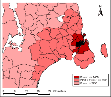
The project was funded and done in collaboration with COPSAC study group. More details about COPSAC cohort can be found at their website http://www.copsac.dk/.

2 Data

2.1 The COPSAC Cohort
2.2 Air Pollutants
2.3 Meteorological Data

Data for this project include the COPSAC cohort, which provided data on the incidence of respiratory symptoms in small children, air pollution data and meteorological data provided by the Danish National Environmental Institute (DMU), and Influenza epidemics data provided by Staten's Serum Institute (SSI).

2.1 The COPSAC Cohort

The COPSAC (COpenhagen Prospective Study on Atopy in Children) cohort was designed to study childhood asthma, eczema and allergy with focus on epidemiological, clinical, cellular and molecular research with consideration to environment and lifestyle factors. COPSAC is unique as it consists of a large group of high-risk children and has long-term continuous data registration. Clinical data are collected prospectively, and biological materials collected into a data bank, which enables par clinical analysis during, before, and after disease development. COPSAC is therefore a unique resource for studying causes and development (course) of asthma, eczema and allergy in children. Details about design of the COPSAC cohort are published elsewhere (Bisgaard, 2004).

The COPSAC cohort consists of 411 children genetically predisposed to atopic illnesses (children of mothers with asthma) living in Denmark. COPSAC children were enrolled in the study at birth and followed until 3 years of age. The first child was enrolled in the cohort on 02.08.1998 and the latest on 29.12.2001. Daily registration of airways symptoms via dairies is carried out by parents for all three years. The presence of the registered symptoms (ICD-10 diagnosis R068) is the outcome in this study. R068 diagnosis includes airways symptoms such as wheezing, apnoeic episode, breath-holding attacks, etc. R068 diagnoses were defined by their starting and finishing date. Most children had R068 diagnoses that lasted more than one day.

For this project, data on incidence of respiratory disease in COPSAC children up to 18 months of age are available. Due to study design where air pollution data are available from a single measuring station located in the centre of Copenhagen (HCØ Institute), three populations of COPSAC children were created according to their home vicinity to the HCØ. By this design it is assumed that air pollution exposure from central monitoring station is most representative exposure for children living in the centre of the city defined by postal code 2450. This, Population 1, is thus the primary study population. Further, Populations 2 and 3 are created, representing those who live in Copenhagen suburbs (2450 < and 2930) and those living in rest of Sealand (2930 < and 5000), as illustrated in Figure 2.1.1. These three populations allow us to study a geographical gradient of centrally measured air pollution's effect on the development of respiratory symptoms in small children, with a hypothesis that this exposure has strongest effect on children living in the centre of the city and this effect gradually diminishing further away from the Copenhagen city centre into the rural areas of Sealand. Geographical distribution of COPSAC children and definition of three populations according to children's' home address postal code can be seen in Table 2.1.1 below. A number of children changed their home address during the first 18 months of life, due to which those children fall into two or all three populations at the different relevant time periods, and the totals do not add up to 411.

Table 2.1.1: Definition of study populations according to postal code of COPSAC children's home address

Figure 2.1.1: Postal code area definition of the three study populations

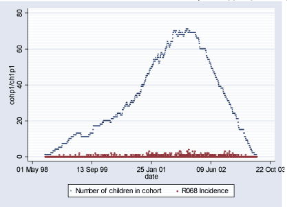
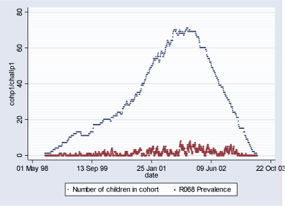
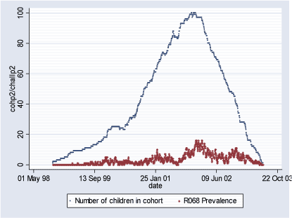
Population 1 consists of 115 children who during some of or the whole period of their first 18 months of life lived in Inner City of Copenhagen (postal code 2450). The follow-up period starts with the earliest child's birthrate 16.08.1998 and ends with the latest 18-month follow-up date on 29.06.2003 totaling in 1.779 days. During this period total of 346 new (incident) cases of R068 diagnoses were observed and 2.332 total (prevalent) cases. Table 2.1.2 and Figures 2.1.2 and 2.1.3 below describe Population 1.

Table 2.1.2: Population 1 - Definition of the outcome

Figure 2.1.2: Daily count of incident cases and number of children in COPSAC Cohort in Population 1 during study period (16.08.1998-29.06.2003)

Figure 2.1.3: Daily count of prevalent cases and number of children in COPSAC Cohort in Population 1 during study period (16.08.1998-29.06.2003)

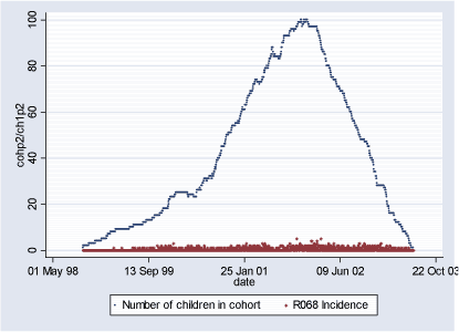
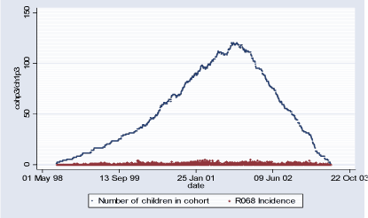
Population 2 consists of 134 children who during some of or the whole period of their first 18 months of life lived in the suburbs of Copenhagen (2450 < postal code 2930). The follow-up period starts with the earliest child's birthrate 06.10.1998 and ends with the latest 18-month follow-up date on 28.06.2003 totaling in 1.727 days. During this period total of 691 new (incident) cases of R068 diagnoses were observed and 5.663 total (prevalent) cases. Table 2.1.3 and Figures 2.1.4 and 2.1.5 describe Population 2.

Table 2.1.3: Population 2 - Definition of the outcome

Figure 2.1.4: Daily count of incident cases and number of children in COPSAC Cohort in Population 2 during study period (06.10.1998-28.06.2003)

Figure 2.1.5: Daily count of prevalent cases and number of children in COPSAC Cohort in Population 1 during study period (06.10.1998-28.06.2003)

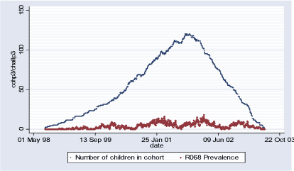
Population 3 consists of 186 children who during some of or the whole period of their first 18 months of life lived in the rest of Sealand (2930 < postal code 5000). The follow-up period starts with the earliest child's birthrate 02.08.1998 and ends with the latest 18 month follow-up date on 22.06.2003 totaling in 1.786 days. During this period total of 914 new (incident) cases of R068 diagnoses were observed and 7.098 total (prevalent) cases. Table 2.1.4 and Figures 2.1.6 and 2.1.7 describe Population 3.

Table 2.1.4: Population 3 – Definition of the outcome

Figure 2.1.5: Daily count of incident cases and number of children in COPSAC Cohort in Population 3 during study period (02.08.1998-22.06.2003)

Figure 2.1.6: Daily count of prevalent cases and number of children in COPSAC Cohort in Population 3 during study period (02.08.1998-22.06.2003)

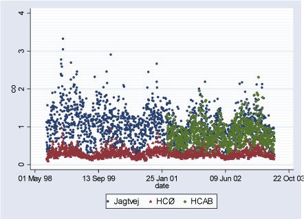
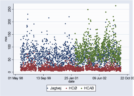
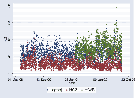
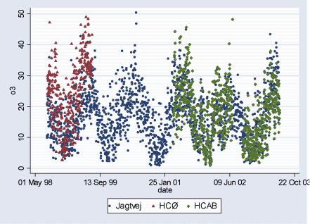
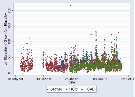
2.2 Air Pollutants

Air pollutant data are available as daily averages of air pollutant levels from following measuring stations in Copenhagen: HCØ Institute (city background pollution levels), Jagtvej and H.C.Andersen's Boulevard (HCAB) (street level pollution levels). From all measuring stations measurements are available for the following pollutants: CO (ppm), NO_x (ppb), NO₂ (ppb), O₃ (ppb), PM₁₀ (g/m³), and TON (part./m³). PM₁₀ at street level measuring stations Jagtvej and HCAB was measured by SM200 gravimetric method. PM₁₀ city background level variable (HCØ) is combined with PM₁₀ measurements from HCØ (SM200 gravimetric method) and values extrapolated from PM₁₀ measurements at Jagtvej (beta method), corrected for traffic contribution using NO_x measurements from HCØ and Jegtvej and the ratio 0.144*(PM₁₀ /NO_x). The extrapolation of PM₁₀ values was done for the study periods where HCØ measurements were missing, to obtain more complete variable. Furthermore, PM_2.5 (µg/m³) measurements are available from HCAB measuring station, and PM₁₀ (g/m³) measurements (SM200 gravimetric method) from Lille Valby (rural Zealand pollution levels). Three high PM₁₀ values measured at HCØ were excluded (176.6 g/m³ on 01.01.2000, 248.5 g/m³ on 01.01.2001, and 283.7 g/m³ on 10.08.2000). Furthermore, a PM₁₀ value of 215.5 g/m³ measured at Jagtvej on 01.01.2001 was excluded. Description of air pollutants can be seen in Table 2.2.1 below, and Figures 2.2.1-2.2.7. Pearson correlation coefficients between pollutants measured at the same station can be seen in Tables A.1 - A.3 in Appendix A.

Table 2.2.1: Air pollutant levels during study period

Figure 2.2.1: CO (ppm) daily levels during study period (02.08.1998-29.06.2003)

Figure 2.2.2: NO_x (ppb) daily levels during study period (02.08.1998-29.06.2003)

Figure 2.2.3: NO₂ (ppb) daily levels during study period (02.08.1998-29.06.2003)

Figure 2.2.4: O₃ (ppb) daily levels during study period (02.08.1998-29.06.2003)

Figure 2.2.5: PM₁₀ (g/m³) daily levels during study period (02.08.1998-29.06.2003)

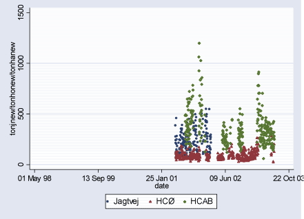
Figure 2.2.6: TON(part./m³)/100 daily levels during study period (02.08.1998-29.06.2003)

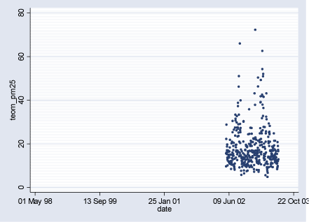
Figure 2.2.7: PM_2.5 (g/m³) daily levels measured at HCAB during study period (02.08.1998-29.06.2003)

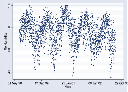
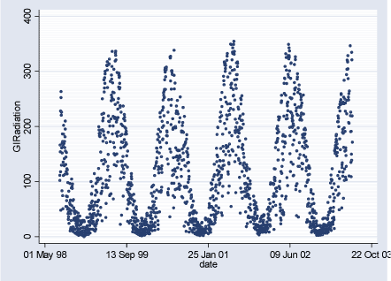
2.3 Meteorological Data

Meteorological data are available as daily hour averages measured at HCØ and include: wind speed (m/s), temperature (C), relative humidity (%), and global radiation (W/m²). Description of meteorological data can be seen in the Table 2.3.1 and Figures 2.3.1 – 2.3.4 below. Pearson correlation coefficients between meteorological variables can be seen in Table 2.3.2. Pearson correlation coefficients between air pollutants measured at HCØ and weather variables can be seen in Table A.4 in Appendix A.

Gennemsnit m.h.t. vindhastighed, temp og fugtighed er vel uinteressant, her er fx kvartiler vel mere beskrivende.

Table 2.3.1: Meteorological data level during study period

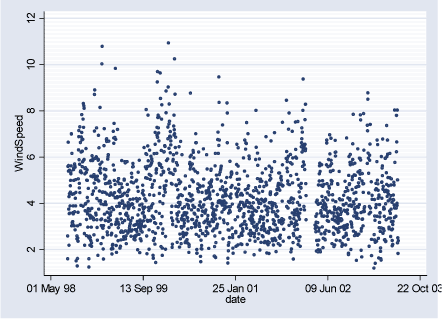
Figure 2.3.1: Wind Speed daily averages during the study period (02.08.1998-29.06.2003)

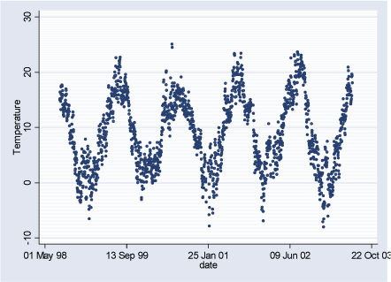
Figure 2.3.2: Temperature daily averages during the study period (02.08.1998-29.06.2003)

Figure 2.3.3: Relative Humidity daily averages during the study period (02.08.1998-29.06.2003)

Figure 2.3.4: Global Radiation daily averages during the study period

Table 2.3.2: Correlation of meteorological variables during the study period in Copenhagen (02.08.1998 - 29.06.2003)

* p < 0.01 - significance level for the Pearson correlation coefficients

In the Table 2.3.2 above it can be seen that there is statistically significant positive association between wind speed and relative humidity, and temperature and global radiation. There is negative and statistically significant correlation between wind speed and temperature, wind speed and global radiation, temperature and relative humidity and global radiation and relative humidity. This table shows that all meteroloigcal variables are mutually correlated, which implies that fitting them in the model together could cause some colinearity. Therefore, we chose only temperature in the final model, as the strongest predictor of the incident respiratory cases in small children.

3 Statistical Methods

3.1 Generalized Additive Model (GAM)
3.2 Modelling Lag Structure

3.1 Generalized Additive Model (GAM)

A generalized additive Poisson regression model was fit modeling the logarithm of the expected value of daily counts of respiratory symptoms as a sum of linear and smooth functions of the predictor variables (Hastie et al., 1990; Schwartz, 1996). The generalized additive model allows regressions to include nonparametric smooth functions to model the potential nonlinear dependence of the daily respiratory symptoms on weather and season. The model assumes:

where Y is the daily count of respiratory symptoms in COPSAC children, E(Y) is the expected value of that count, X_i is the covariate, and S_i is the smooth function. For the Si we used smoothing spline. This approach is standard in air pollution time-series modeling (Schwartz, 1994).

Smoothing spline is a type of smoother, which is a nonparametric tool for summarizing the trend of a response measurement Y as a function of a predictor measurements X. Smoothers serve as a descriptive tool, depicting the shape of a relationship between X and Y, and as a building block of the estimation of additive models. The simple example of a smoother is a running mean (or moving average), while others types of smoothers include polynomial, loess, Gaussian kernel, regression spline, natural spline, etc. Smoothing spline creates a smooth curve through the data, where the level of smoothness is adjusted by a varying parameter that changes the curve from a least squares-line Approximation to a cubic spline interpolant. The smoothing spline s is constructed for the specified weights wi . The smoothing spline minimizes

If the weights are not specified, they are assumed to be 1 for all data points. p is defined between 0 and 1, p = 0 produces a least squares straight line fit to the data, while p = 1 produces a cubic spline interpolant. When non-specified, the smoothing parameter is automatically selected within `interesting range' near 1/(1+h³/6) where h is the average spacing of the data points, and is tipically much smaller than the allowed range of the parameters. Because smoothing splines have an associated parameter, these fits can be considered to be parametric. However, smoothing splines are also piecewise polynomials like cubic splines or shape-perserving interpolants and are thus most often considered a nonparametric fit type.

Our final model was:

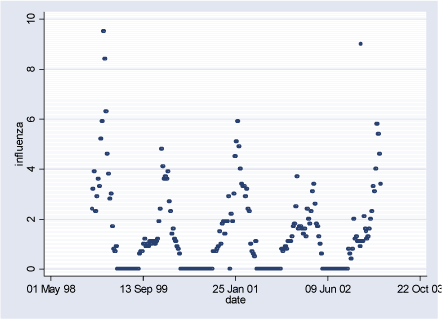
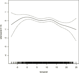
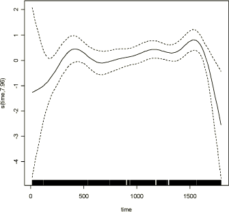
where Y_t denotes the daily count of new respiratory symptoms (incidence) in COPSAC children, assumed to be Poisson distributed, β₁ denotes the log relative rate of morbidity associated with an unit increase in mean daily pollution, P_t pollutant of interest, S₂(T,5) is a smooth function of temperature with 5 degrees of freedom, S₃(time,8) a smooth function of time with 8 degrees of freedom, and offset(log(cohort)) term that incorporates weighing the daily number of new respiratory symptoms over the daily number of children in the cohort.

Single pollutant model was fit for each of the pollutants in Table 2.2.1, for all three populations defined in the section 2.1. Missing values were excluded from the analysis. Each pollutant was treated as having linear association with respiratory symptoms. To reduce sensitivity to outliers in the pollution levels the analysis excluded extremely high values. Exclusion of the extreme values was described in section 2.2.

The daily count of incident (new) cases of respiratory symptoms in COPSAC children was the main outcome in the study as registered on the first day of the event. A pilot study was performed with counts of prevalent cases in Population 1 and 2 together, and lead to the conclusion that incidence is most relevant clinical outcome in this study. Prevalence of symptoms on a given day would be highly dependent on prevalence of symptoms in the subject on the previous day and prevalence would be difficult to interpret with respect to lag-time in relation to air pollution levels.

Smoothing functions were used to capture seasonal and other short-term and long-term trends in the data. Temperature was used to capture potential short-term confounding. Other meteorological variables did not enter the final model due to correlation with temperature (Relative Humidity) or non significance (Wind Speed and Global Radiation). Smooth functions of time were used to remove the basic long-term pattern in the data. The span for the smooth function of time was chosen to remove seasonal and long-term trends and to minimize autocorrelation in the residuals, by methods described previously (Schwartz, 1999). The day of the week indicator, a standard variable used in GAM models to capture short-term trends, was not significant confounder in this study. Influenza epidemics variable, defined as a weekly percent of total physician visits, was not significant confounder in this study (Appendix B).

Analyses were performed by gam function, mgcv package in R statistical software.

3.2 Modelling Lag Structure

To evaluate the impact of air pollutants for up to 5 days after exposure several lag modeling methods were implemented. We chose a maximum lag of 5 days before the respiratory symptom incidence for the air pollution variable, because the goal of this analysis is to estimate the short-term effects of air pollution, and because previous studies have shown that longer lag had little correlation with development of respiratory symptoms.

Distributed lag models have been commonly used in social sciences and recently implemented in epidemiology by Pope and Schwartz (Judge et al., 1980; Pope et al., 1996). The motivation for the distributed lag model is the realization that air pollution can affect the development of respiratory symptoms in children not only on the same day but also on several consequent days. Unconstrained distributed lag model assumes:

where Xt-is the pollutant concentration q days before the occurrence of respiratory symptom. The overall effect of a unit increase in air pollution on a single day is its impact on that day plus that on subsequent days, that is sum of 0+ . . .+ q. Thus equation above can be rewritten as:

where the ω_i are weights that sum to 1, and β* is β₀+ . . .+ β_q. That is, β* is interpretable as the marginal effect of a unit increase in a weighted average pollution variable. Because a unit increase in pollution on a single day increases the weighted average on all subsequent days, the effect of that single day's increase will be β*ωi on each of the q subsequent days, or β* overall.

We fit unconstrained distributed lag model adapted to the GAM model from section 3.1:

where P_t is the air pollution level on the day t of the incidence occurrence, and P_t-5 is the air pollution level 5 days prior to incidence occurrence.

Because there is a substantial correlation between air pollution concentrations on the days close together, the above regression may have a high degree of colinearity, that results in unstable, but unbiased estimates of β's.

Next, to gain more insight into the shape of the distribution of the effect over lag, we fit single day's air pollutant exposure model, where pollutant level at day t and on subsequent days for up to 5 days are fit separately. This is an alternative approach to the unconstrained distributed lag model which is a constrained lag model, with a very restrictive constrain where β₁= β₂ = . . .= β_q=0. As we are not quite sure that the effects of pollution are limited to a single day, these constraints are much more restrictive than those in the undistributed lag model, and are likely to introduce bias in the estimated overall effect. They, however, give a marginal effect of a single day exposure and thus provide useful insight into the shape of the distribution of the effect over lag.

We finally also fit a traditional moving average approach with a 6-day moving average, to compare overall effect estimates with those from undistributed lag model.

4 Results

4.1 Population 1 - Inner City Copenhagen
4.2 Population 2 - Copenhagen Suburbs
4.3 Population 3 - Rest Of Zealand

Results are presented separately for three study populations defined in Section 2.1. Each table presents estimated effect of a unit increase in a pollutant using the GAM model (Section 3.1) with three lag modeling methods: single day exposure lag model, the unconstrained distributed lag model, and the 6-day moving average (Section 3.2). Each table presents results for a single pollutant, from all measuring stations available for that pollutant. Effect of confounders, temperature and time, are presented elsewhere (Appendix D).

4.1 Population 1 – Inner City Copenhagen

From Table 4.1.1, 6-day moving average results indicate that Copenhagen city background levels of CO are positively but not significantly associated with development of respiratory symptoms in COPSAC children living in inner city, while street level concentrations of CO are significantly positively associated with the outcome. An increase in 1 ppm in 6-day average CO measured at street level (Jagtvej and HCAB) is associated with 1.89 fold and 3.11 fold (with wide confidence intervals) increase respectively in in new cases of respiratory children living in Copenhagen inner city the following

Table 4.1.1: CO (ppm) effect in Population 1

days. Estimates from a single day exposure lag models and unconstrained distributed lag model, indicate for all, background and street levels, that concurrent day pollution has weak effect on the development of the symptoms on the same day, but that effect increases and lasts over several days, peaking at around 2 (street levels) or 3 (background levels) days delay.

Table 4.1.2: NO_x (ppb) effect on Population 1

RR - relative risk; - regression coefficient; se - standard error of the regression coefficient; p – significance level of the regression coefficient

In Table 4.1.2, 6-day average results indicate that Copenhagen city background levels of NO_x are positively and borderline significantly associated with development of respiratory symptoms in COPSAC children living in inner city, whereas the association is significant in one street station. A unit increase in 6-day average city background NO_x pollution levels results in 1.9 % increase in new respiratory cases the next day, while a unit increase in 6-day average street level NO_x pollution at Jagtvej and HCAB results in 0.6% and 1.3% increase in new respiratory cases the next day respectively. Looking at estimates from a single day exposure lag model and unconstrained distributed lag models, for all, background and street levels, it can be seen that concurrent day pollution has weak or no effect on the development of the new respiratory symptoms. This effect is increasing with a few days' delay, that seems to be strongest with a 3-day delay at city background levels, and 2-day delay at street levels.

In Table 4.1.3, 6-day average results indicate that there is positive but no significant association between Copenhagen city and street level NO₂ pollution levels and development of respiratory symptoms in COPSAC children living in inner city. Looking at estimates from a single day exposure lag model and unconstrained distributed lag models, for background and street NO₂ levels, it can be seen that concurrent day pollution has weak or no effect on the development of the new respiratory symptoms, but as seen in NO_x, this effect is increasing with a delay, that seems to be strongest with a 2-day delay.

Table 4.1.3: NO₂ (ppb) effect on Population 1

RR - relative risk; - regression coefficient; se - standard error of the regression coefficient; p – significance level of the regression coefficient

In Table 4.1.4 can be seen that Copenhagen city background O₃ is positively but not significantly associated with development of respiratory symptoms in COPSAC children living in inner city. This effect seems to be strongest after 2-day lag. However, Copenhagen city street level O₃ is negatively associated with the outcome, with this protective effect being more or less constant over the 5 days. Thus, a 1 ppb increase in 6-day average Jagtvej and HCAB O₃ levels is associated with a 2% and 4.5% decrease in new respiratory cases in children the following days.

Table 4.1.5 shows that the incidence of new respiratory symptoms is positively and borderline significant with respect to the 6-day moving average model associated with the Copenhagen city background levels of PM₁₀. The estimate indicate that a 1 /m³ increase in 6-day average PM₁₀ Copenhagen city background levels results in 1% increase in development of new respiratory symptoms in children living in inner city the next 5 days. Estimates from a single day exposure lag model and unconstrained distributed lag models indicate that the effect is delayed with the strongest effect after 3 or 4 days.

Table 4.1.4: O₃ (ppb) effect on Population 1

RR - relative risk; - regression coefficient; se - standard error of the regression coefficient; p – significance level of the regression coefficient

Table 4.1.5: PM₁₀ (µg/m³)(combined with HCØ measurements and extrapolated values from Jagtvej) effect on Population 1

RR - relative risk; - regression coefficient; se - standard error of the regression coefficient; p – significance level of the regression coefficient

Table 4.1.6 shows that there is a positive but non-significant association between both, street level (Jagtvej) and rural level (Valby) PM₁₀ and incidence of respiratory illness in small children living in inner city. The distributed lag models indicate, in agreement with city background PM₁₀ results, that this association is strongest after 3 to 4 day lag.

Table 4.1.6: PM₁₀ (µg/m³) (measured by SM200 gravimetric method) effect on Population 1

RR - relative risk; - regression coefficient; se - standard error of the regression coefficient; p – significance level of the regression coefficient

Table 4.1.7 shows that, according to a 6-day moving average model, there is negative and no significant association between HCAB street level ultrafine particles PM_2,5 and respiratory disease incidence in small children living in inner city of Copenhagen. However, single day exposure lag model points at strong positive association with some delay of from 2 to 4 days. Unconstrained distributed lag model points at positive association at 2-day lag. Note that this analysis is limited by a small amount of PM_2.5 data.

Table 4.1.7: PM_2.5 (µg/m³) (measured by SM200 gravimetric method) effect on Population 1

RR - relative risk; - regression coefficient; se - standard error of the regression coefficient; p – significance level of the regression coefficient

Table 4.1.8 shows that there is no significant effect of neither, Copenhagen city background or street TON (part. /m³) levels on the incidence of respiratory disease in small children living in Copenhagen inner city. The estimates presented in the table are multiplied by 100. The 6-day average moving average model indicate no or a negative association between TON city background levels and the development of respiratory symptoms, but results from single day exposure lag model and unconstrained distributed lag model indicate positive association at 4-day lag. The street TON levels show a positive non-significant association to the outcome with a 3-day lag for Jagtvej. Note that analyses with TON are based on a limited amount of available data.

Table 4.1.8: TON (part./m³) (x100) effect on Population 1

RR - relative risk; - regression coefficient; se - standard error of the regression coefficient, p - p value

4.2 Population 2 – Copenhagen Suburbs

From Table 4.2.1, 6-day moving average results indicate that Copenhagen city background levels of CO are not or if anything negatively associated with development of respiratory symptoms in COPSAC children living in Copenhagen suburbs, while street level concentrations of CO are positively but far from significantly associated with the outcome. Estimates from a single day exposure lag model and unconstrained distributed lag models, indicate that, consistently for all, background and street levels, positive association with the outcome may appear with 4-day lag.

Table 4.2.1: CO (ppm)

RR - relative risk; - regression coefficient; se - standard error of the regression coefficient; p – significance level of the regression coefficient

In Table 4.2.2, 6-day moving average results indicate that Copenhagen city background levels of NO_x are not associated with development of respiratory symptoms in COPSAC children living in Copenhagen suburbs, while street level concentrations of NO_x are positively but not significantly associated with the outcome. Estimates from a single day exposure lag model and unconstrained distributed lag models, indicate that consistently for all, background and street levels, positive effect on the outcome is strongest at 4-day lag.

Table 4.2.2: NO_x (ppb)

RR - relative risk; - regression coefficient; se - standard error of the regression coefficient; p – significance level of the regression coefficient

Table 4.2.3 show that the NO₂ levels Copenhagen city background and streets are only weakly and far from significantly with respect to 6-day average associated with development of respiratory symptoms in COPSAC children living in Copenhagen suburbs. Estimates from a single day exposure lag model and unconstrained distributed lag models points to possible positive associations with 3-4 days lag.

Table 4.2.3: NO₂ (ppb)

RR - relative risk; - regression coefficient; se - standard error of the regression coefficient; p – significance level of the regression coefficient

In Table 4.2.4 it can be seen that 6-day average of all, Copenhagen city background and street O₃ levels are mainly negatively but far from significantly associated with development of respiratory symptoms in COPSAC children living in Copenhagen suburbs. Estimates from a single day exposure lag model and unconstrained distributed lag models confirm the weak associations and show no obvious lag patterns.

Table 4.2.5 shows that there is negative although not significant associations between Copenhagen city background PM₁₀ levels and increase in development of new respiratory symptoms in children living in Copenhagen suburbs with the 6-day moving average model. This weak association holds for the same day and delayed effects, without obvious lag patterns.

Table 4.2.4: O₃ (ppb)

RR - relative risk; - regression coefficient; se - standard error of the regression coefficient; p – significance level of the regression coefficient

Table 4.2.5: PM₁₀ (µg/m³), combined with HCØ measurements and extrapolated values from Jagtvej

RR - relative risk; - regression coefficient; se - standard error of the regression coefficient; p – significance level of the regression coefficient

Table 4.2.6: PM₁₀ (g/m³) measured by SM200 gravimetric method

RR - relative risk; - regression coefficient; se - standard error of the regression coefficient; p – significance level of the regression coefficient

In Table 4.2.6, similarly to results for city background levels of PM₁₀ (Table 4.2.5), it can be seen that there is no significant effect of Copenhagen street (Jagtvej) or rural (Lille Valby) PM₁₀ levels on the respiratory disease incidence in small children living in Copenhagen suburbs, with non-significant negative association and no obvious lag patterns

Table 4.2.7: PM_2,5 (µg/m³) effects on Population 2

RR - relative risk; - regression coefficient; se - standard error of the regression coefficient; p – significance level of the regression coefficient

There is no significant association between Copenhagen street level (HCAB) ultra fine particle level PM_2,5 and respiratory disease incidence in small children living in Copenhagen suburbs as it can be seen in Table 4.2.7.

Table 4.2.8: TON (part./m³) (x100)

RR - relative risk; - regression coefficient; se - standard error of the regression coefficient; p – significance level of the regression coefficient

Table 4.2.8 shows that there is no significant association between neither Copenhagen city background nor street TON (part./m³) levels and the incidence of respiratory disease in small children living in Copenhagen suburbs. The estimates presented in the table are multiplied by 100. An association may be negative, in particularly, with respect to the city background levels.

4.3 Population 3 – Rest Of Zealand

From Table 4.3.1, 6-day moving average results indicate that Copenhagen city background and street levels of CO are positively but not significantly associated with development of respiratory symptoms in COPSAC children living in the rest of Sealand. Looking at estimates from a single day exposure lag model and unconstrained distributed lag models, it can be seen that at all, background and street levels, positive effect on the outcome is strongest at 2-day lag.

In Table 4.3.2, 6-day moving average results indicate that Copenhagen city background and street levels of NO_x are positively non-significantly associated with development of respiratory symptoms in COPSAC children living in the rest of Zealand. Looking at estimates from a single day exposure lag model and unconstrained distributed lag models, it can be seen that, positive associations may be present and strongest at around 2-day lag.

Table 4.3.3 shows that according to 6-day average results there is positive but nonsignificant association between Copenhagen city background and street levels (HCAB) of NO₂ and development of respiratory symptoms in COPSAC children living in the rest of Sealand, while this association is positive at city street levels from Jagtvej (increase in 1 ppb of 6-day average NO₂ levels resulting in 1.7% increase in new respiratory symptoms cases the following days). Estimates from a single day exposure lag model and unconstrained distributed lag models, indicate that for all, background and street levels of NO₂, positive the association with the outcome is strongest at a 2-day lag.

Table 4.3.1: CO (ppm)

RR - relative risk; - regression coefficient; se - standard error of the regression coefficient; p – significance level of the regression coefficient

In Table 4.3.4 can be seen that Copenhagen city background O₃ is negatively but far from significantly associated with development of respiratory symptoms in COPSAC children living in the rest of Zealand. However, Copenhagen city levels of O₃ are significantly negatively associated with the outcome. Thus, a 1 ppb increase in 6-day average Jagtvej and HCAB O₃ levels is associated with a 2.6% and 1.5% decrease in new respiratory symptoms in children the following days.

Table 4.3.5 shows that there is no effect of Copenhagen city background levels of PM₁₀ and development of new respiratory symptoms in children living in the rest of Zealand.

Table 4.3.2: NO_x (ppb)

RR - relative risk; - regression coefficient; se - standard error of the regression coefficient; p – significance level of the regression coefficient

In Table 4.3.6, similarly to results for Copenhagen city background levels of PM₁₀ (Table 4.3.5), it can be seen that there is no significant effect of street level (Jagtvej) or rural levels (Lille Valby) PM₁₀ levels on the respiratory disease incidence in small children living in the rest of Zealand, with negative association and no obvious lag patterns.

Table 4.2.8 shows that there is no significant effect of Copenhagen city background or street TON (part./m³) levels on the incidence of respiratory disease in small children living in the rest of Zealand. The estimates presented in the Table 4.3.8 are multiplied by 100.

Table 4.3.3: NO₂ (ppb)

RR - relative risk; - regression coefficient; se - standard error of the regression coefficient; p – significance level of the regression coefficient

Table 4.3.4: O₃ (ppb)

RR - relative risk; - regression coefficient; se - standard error of the regression coefficient; p – significance level of the regression coefficient

Table 4.3.5: PM₁₀ (µg/m³) , combined with HCØ measurements and extrapolated values from Jagtvej

RR - relative risk; - regression coefficient; se - standard error of the regression coefficient; p – significance level of the regression coefficient

Table 4.3.6: PM₁₀ (µg/m³) measured by SM200 gravimetric method

RR - relative risk; - regression coefficient; se - standard error of the regression coefficient; p – significance level of the regression coefficient

Table 4.3.7: PM_2,5 (µg/m³)

RR - relative risk; - regression coefficient; se - standard error of the regression coefficient; p – significance level of the regression coefficient

Table 4.3.8: TON (part./m³) (x100)

RR - relative risk; - regression coefficient; se - standard error of the regression coefficient; p – significance level of the regression coefficient

5 Discussion and Conclusion

We find consistent associations between daily ambient levels of air pollutants and daily incidence of respiratory symptoms in terms of wheezing during the first 18 month of life of children with atopic predisposition and living in Copenhagen. Among children from central Copenhagen the associations were statistically significant and positive with respect to street levels of CO and NO_x, and negative with respect to street levels of O₃, whereas positive associations with urban background levels of PM₁₀, CO and NO₂ were borderline significant. Among children living in Copenhagen suburbs or the rest of Zealand similar but much weaker associations with the gases were seen, only significant for street levels of NO₂ and O₃ at one station and only for children from outside Copenhagen, whereas there were no associations with PM₁₀ levels. These apparently differential associations related to distance from the sources of pollutants and monitoring sites supports causal relationships. Moreover, positive associations with the street levels of CO and NO_x and negative with street levels of ozone, which is consumed by NO from diesel emission, suggest traffic as the important source of pollutants relevant for airway symptoms. Associations with total number concentrations of ultrafine particles, which are mainly traffic generated, would also be expected, although these were not significant, but that may be due to the low number of days with measurements. We find furthermore that air pollution has small or no effect on development of the outcome on the concurrent day, but that the effect on airway symptoms comes with a delay of 2-4 days for different pollutants and that the effect is accumulated over several days.

An increase in 1 ppm in 6-day average CO measured at street level (Jagtvej and HCAB) is associated with 1.89 fold and 3.11-fold (with wide confidence intervals) increases in new cases of respiratory symptoms in small children living in Copenhagen inner city the following days, respectively (Table 4.1.1). Note that CO levels are measured in ppm and that 1 ppm corresponds to a little more than a doubling of average levels at Jagtvej and HCAB of 0.99 and 0.81 ppm, respectively. Associations with CO levels measured in city background are borderline significant (p=0.10) and it points at an almost 5-fold increase in respiratory disease incidences in small children the day after 6-day average CO pollution increase by 1 ppm. We find finally that concurrent day pollution has weak effect on the development of the symptoms on the same day, but that effect increases and lasts over several days, peaking at around 2 (street levels) or 3 (background levels) days delay. CO is not an irritant gas and it is unlikely to be causative in development of respiratory symptoms. However, CO is mainly emitted by gasoline powered vehicles and can be considered as an indicator of traffic. The levels of CO correlate very closely with NO_x and TON at the street stations (r>0.82), the correlations with NO_x are particularly strong (r>0.91). The relevance of the associations among children form central Copenhagen is supported by much weaker and non significant associations between CO in central Copenhagen and outcome among small children living farther away in Copenhagen suburbs (Table 4.2.1) and the rest of Zealand (Table 4.3.1).

A unit increase (1 ppb) in 6-day average city background NO_x pollution levels is associated with a 1.9 % (borderline significant) increase in new respiratory cases the following days, while a unit increase in 6-day average street level NO_x pollution at Jagtvej and HCAB results in 0.6% and 1.3% (significant) increases in new respiratory cases the next day respectively. Note that a 1 ppb increase corresponds to 7%, 1.6% and 1% increases from daily average levels of 15, 61 and 87 ppb at the city background, Jagtvej and HCAB monitoring stations, respectively. Thus, a doubling of the average levels at the city background, Jagtvej and HCAB monitoring stations would correspond to 29%, 37% and 113% increases in the outcome, respectively. This apparent effect occurs with a few days' delay, that seems to be strongest with a 3-day delay at city background levels, and 2-day delay at street levels. The associations of respiratory symptoms among children from central Copenhagen with monitoring station levels of NO₂ show a pattern similar to that of NO_x although with considerably higher but non-significant effect estimates, and similar 2-day lag. Similar positive but much weaker and non significant associations were found for symptoms and NO₂ and NO_x in the children living outside central Copenhagen a 2-day lag for city background measurements and less clear lag patterns for street level measurements, supporting the relevance of the associations in central Copenhagen. Levels of NO_x and NO₂ have previously been associated with the daily count of house calls related to upper and lower airway symptoms among Copenhagen children (Keiding et al. 1995). NO_x is the sum of NO and NO₂. NO is emitted in particular from diesel vehicles and reacts readily with available ozone to form NO₂. Thus, the levels of NO₂ are only a third of the NO_x at the street monitoring stations, whereas there is only a small difference between NO₂ (11.9 ppb) and NO_x (15.5 ppb) in city background and the correlation between them is stronger (r: 0.92) than at the street stations (r: 0.80 and 0.83). However, NO₂ is the gas with airway irritant properties whereas NO is generated in the human body and has e.g. vasoactive properties and neurosignialling properties. Several cohort studies have shown increased risk of persistent cough and shortness of breath among infants with high NO₂ levels in the home (van Strien et al.. 2004). Similarly, a Swedish nested in cohort case-control study showed that high NO₂ levels measured outside the dwelling of children aged up to two years were associated with increased risk of recurrent wheezing (Emenius et al. 2003). The only published panel based time-series study of infants similar to our study did not show consistent associations between daily incidence of wheezing bronchitis and NO₂, whereas no data for NO_x were reported (Pino et al. 2004). In a population based study in a part of London there was a non-significant association between daily NO₂ levels and daily counts of emergency room visits with wheezing among infants, whereas ozone levels and some hydrocarbons showed significant associations (Buchdahl et al. 2000). Accordingly, the present statistically stronger association between the respiratory outcome and NO_x than with respect to NO₂ and also the more clear association with street levels rather than city background levels could also suggest that the associations are not directly causal. NO_x levels could be an indicator of traffic generated air pollution e.g. in terms of ultrafine particles and it is closely correlated with TON at the street stations (r: 0.95 at Jagtvej and 0.76 at HCAB).

An apparently protective effect of O₃ on development of respiratory symptoms in COPSAC children is consistent across all three populations, except for city background measurements in central Copenhagen children, where we see positive non significant association. The apparent protective effect of O₃ measured at street level is significant in children from central Copenhagen and from Zealand beyond Copenhagen suburbs (pulations 1 and 3). This may be surprising because ozone is known as a strong airway irritant associated with e.g. incidence of asthma and airway symptoms (Buchdahl et al. 2000; McConnel et al. 2002). However, the levels are relatively low in Denmark and the apparently protective effect may be related to consumption of ozone by NO emitted from diesel vehicles, supporting that traffic generated air pollution could be responsible for the association with respiratory symptoms. Indeed, ozone is negatively correlated (r-values around -0.7) with CO and NO_x at both urban background and street monitoring stations.

Result from the moving average model for PM₁₀ for Copenhagen city background levels indicate positive but borderline significant (p=0.07) associations with new respiratory symptoms in children living in inner city, with the strongest effect after 3- to 4- days lag, where the associations were significant in the single day exposure lag model (Table 4.1.5). The effect estimate of a 1% increase in incidence of symptoms for a 1 µg/m³ increase in PM₁₀ is completely consistent with findings from Santiago, Chile (Pino et al. 2004). There, a 1% increase in wheezing bronchitis for 1 µg/m³ increase in PM_2.5 with a lag time of 2 to 10 days was found among 504 children aged 4-12 months in particular among those with predisposition for asthma. In the present study no association with urban background PM₁₀ was seen for the children living in Copenhagen suburbs or the rest of Zealand, nor for the PM₁₀ measured at Jagtvej (street level) and Lille Valby (rural levels), supporting the relevance of the findings. In Santiago, Chile, PM_2.5 was stated to be strongly dependent on traffic, which is not the case in Copenhagen, where long range transport is a main contributor to urban background levels. Nevertheless, urban background PM₁₀ levels are correlated with the traffic generated gases at the background as well as the street monitoring stations with r-values around 0.5. Part of this covariation is probably due to meteorological conditions with low wind speed, inversion and stagnant air favoring persistence of air pollution around the sources of emission. Thus, at present it is difficult to determine which air pollutants are most relevant for the airway symptoms in infants although traffic appears to be important.

The results for PM_2.5 measured at street level (HCAB) indicate weak negative and far from significant associations in all three populations. With the single day exposure model lag findings among children from central Copenhagen are however consistent with the positive association for PM₁₀ where the strongest effect is seen at around 4-day lag (Table 4.1.7). Note that there was limited number of observation for the PM_2.5 analyses.

Analyses with TON (part./cm³) show that there is no significant association with the incidence of respiratory disease in small children in any of the populations of children. For the Jagtvej street station with the unconstrained distributed lag model and with the single day exposure model also for the city background station there are some signs of a positive association with a lag of 3 to 4 days. Note that the analyses with TON are based on a limited amount of available data. TON includes all ultrafine particles both liquid and solid, including soot. The latter may be the most relevant where effect may disappear when all particles are considered. Although, small children with there small airways may be expected to be particularly susceptible to ultrafine particles there are not yet data published to support that notion. In the only available study, which included older children (7-12 years old), with asthma symptoms were associated more closely with PM₁₀ and soot than with ultrafine particles (Pekkanen et al. 1997); whereas ultrafine particles were more closely associated with asthma symptoms in adults patients than fine and coarse particles were (Peters et al. 1997; Pentinen et al. 2001).

The results seen above should be take with some caution due to limitations of our study which include small number of outcomes due to small cohort of asthma susceptible children, large number of missing data for certain pollutants, and multiple testing issues due to large number of available pollutants from several measuring stations. In addition, as explained in Appendix C, our modeling approach where we treat day-to-day outcome as independent, may underestimate standard errors of the estimates and thus lead to overestimated p-values. With further appropriate adjustment for p-values for multiple testing, some of the significant p-values we report may no longer be significant. The small number of outcomes also affects the p-values. However, due to strength of our study of large number of available pollutant data, from several different sources, we get convincingly consistent estimates for pollutants across different measuring stations for the same populations, which validate these associations, and point at their true effect, regardless of significance.

The levels of air pollutants as well as the respiratory symptoms show seasonal and other time-dependent variation and both may be affected be meteorological conditions, which could cause confounding. However, season, day of the week and meteorology were controlled for in our GAM model with relevant smoothing functions, although it cannot be excluded that residual confounding from seasonal variation and/or other unidentified confounders are responsible for the apparent association between lower respiratory symptoms and air pollutant levels. Nevertheless, the apparent differential relationship between outcome and air pollutant levels which were much stronger with dwelling close to the monitoring stations than with dwelling farther away is strongly supportive of relevant associations.

Strengths of our study include a well defined and well characterized birth cohort of 400 susceptible small children followed for 1½ year and a large pool of pollutant data from several different measuring stations. Our study has a unique outcome recorded prospectively. The outcome consists of all R068 symptoms recorded daily into diaries by parents of the children regardless of their origin (asthma, influenza, etc.), where most other studies of air pollution health effects in small children include outcomes based on physician defined diagnoses of asthma, wheezing bronchitis, etc. and focus on one outcome for each child, i.e. diagnosis or not related to a cumulated exposure. That may allow risk of confounding due to other person related factors. Thus, effect estimates are not easily compared except between time-series based studies and here our results compare well with the only other published study by Pino et al. (2004) as described above. A strength of the time-series based design is that the subjects in principle are their own control and only factors with temporal variation give rise to serious risk of confounding.

Our results confirm our hypothesis that children living in central Copenhagen (postcode ≤ 2450) are the most relevant population choice, as it is most representative of pollution levels measured in urban background at in the street at Jagtvej and HCAB. The association between symptoms and in particular CO and NO_x and inverse association with ozone suggest a relationship with traffic related air pollution as there is no other significant sources, where CO is mainly associated with petrol driven cars whereas NO_x is associated with diesel powered vehicles. Thus, ultrafine particles, which are emitted from particularly diesel vehicles, would also be expected to show associations but showed less consistency, Our results for particles were borderline significant for PM₁₀ which have other main sources than traffic, but completely consistent with the only published similar study from Santiago, Chile, where traffic may be more important for fine particles (Pino et al. 2004). Only the data for CO, NO_x and NO₂ are close to complete for the study periods, whereas data on PM₁₀ and ultrafine number concentrations are very incomplete. Thus, lack of significant associations with symptoms may also be related to low statistical power as can be seen from the large standard errors for most of the coefficient estimates.

6 Reference List

Arlian LG, Platts-Mills TA. Thebiology of dust mites and the remediation of mite allergens in allergic disease. J Allergy Clin Immunol 2001;107(Suppl. 3):S406-S413.

Arshad SH, Matthews S, Gant C, Hide DW. Effect of allergen avoidance on development of allergic disorders in infancy. Lancet 1992;339:1493-1497.

Arshad SH, Stevens M, Hide DW. The effect of genetic and environmental factors on the prevalence of allergic disorders at age of two years. Clin Exp Allergy. 1993;23:504-511.

Bates DV, Szito R. The Ontario Air Pollution Study: identification of the causative agent. Environ Health Perspect. 1989;79:69-72.

Berry M, Lioy PJ, Gelperin K, Buckler G, Klotz J. Accumulated exposure to oznone and measurement of health effects in children and counselors at two summer camps. Environ Res. 1991;54:135.150.

Bisgaard H. The Copenhagen Prospective Study on Asthma in Childhood (COPSAC): design, rationale, and baseline data from a longitudinal cohort. Ann Allergy Asthma Immunol. 2004;93:381-389.

Boezen HM, van der Zee SC, Postma DS, et al. Effects of ambient air pollution on upper and lower respiratory symptoms and peak expiratory flow in children. Lancet. 1999;353:874-878.

Braun-Fahrlander C, Ackerman-Liebrich U, Schwartz J, Grehm HP, Rutishausser M, Wanner HU. Air pollution and respiratory symptoms in pre-school children. Am Rev Respir Dis. 1992;145:42/47.

Brunekreef B, Holgate ST. Air Pollution and health. Lancet 2002;360:1233-1242.

Burnett RT, Dales RE, Raizenne ME, et al. Effects of low ambient levels of ozone and sulfates on the frequency of respiratory admissions to Ontario hospitals. Environ Res. 1994;65:172-194.

Dassen W, Brunekreef B, Hoek G, et al. Decline in chidlren's pulmonary function during an air pollution episode. J Air Poll Control Assoc. 1986;36:1123-1127.

Dockery DW, Ware JH, Ferris BG, Speizer FE, Cook NR, Herman SM. Change in pulmonary function associated with air pollution episodes.

Emenius G, Pershagen G, Berglind N, Kwon HJ, Lewne M, Nordvall SL, Wickman M NO₂, as a marker of air pollution, and recurrent wheezing in children: a nested case-control study within the BAMSE birth cohort. J Air Poll Control Assoc. 1982;32:937-942. Occup Environ Med. 2003 Nov;60(11):876-81.

Fisher PH, Steerenerg PA, Smelder JD, Van Loveren H, Van Amsterdam JG. Association between exhaled nitric oxide, ambient air pollution, and respiratory health in school children. Int Arch Occup Environ Health. 2002;75:348-353.

Friedman MS, Powell KE, Hutwagner L, Graham LM, Teague WG. Impact of changes in transportation and commuting behaviors during the 1996 Summer Olympic Games in Atlanta on air quality and childhood asthma. JAMA 2001;285:897-905.

Gauderman WJ, Avol E, Gilliland F, Vora H, Thomas D, Berhane K, McConnell R, Kuenzli N, Lurmann F, Rappaport E, Margolis H, Bates D, Peters J. The effect of air pollution on lung development from 10 to 18 years of age. N Engl J Med. 2004; 351: 1057-67.

Giroux M, Bremont F, Ferrieres J, Dumas JC. Exhaled NO in asthmatic children in unpolluted and urban environments. Environ Int. 2001;27:335-340.

Gold DR, Damokosh AI, Pope CA 3rd, et al. Particulate and ozone pollutant effects on the respiratory function of children in southwest Mexico City. Epidemiology. 1999;10:8-16.

Gold DR. Environmental tobacco smoke, indoor allergens, and childhood asthma. Environ Health Perspect 2000;108:643-651.

Hastie T, Tibshirani R. Generalized Additive Models. London: Chapman and Hall; 1990.

Jalaludin BB, Chey T, O'Toole BI, Smith WT, Capon AG, Leeder SR. Acute effects of low levels of ambient ozone on peak expiratory flow rate in a cohort of Australian children. Int J Epidemiol. 2000;29:549-557.

Kharitonov SA, Yates D, Springall DR, et al. Exhaled nitric oxide is increased in asthma. Chest. 1995;107(3 supl):156S-157S

Keiding LM, Rindel AK, Kronborg D. Respiratory illnesses in children and air pollution in Copenhagen. Arch Environ Health. 1995;50:200-206.

Kinney PL, Lippmann M. Respiratory effects of seasonal exposure to ozone and particles. Arch Environ Health. 2000;55:210-216.

Massaro AF, Mehta S, Lilly CM, Kobzik L, Reily JJ, Drazen JM. Elevated nitric oxide concentrations in isolated lower airway gas of asthmatic subjects. Am J Respir Crit Care Med. 1996;153:1510-1514.

McConnell R, Berhane K, Gilliland F, London SJ, Islam T, Gauderman WJ, Avol E, Margolis HG, Peters JM. Asthma in exercising children exposed to ozone: a cohort study. Lancet 2002;359:386-91.

Medina S, Le Tertre A, Quenel P, et al. Air pollution and doctors' house calls: results from the ERPURS system for monitoring the effects of air pollution on public health in Greater Paris, France 1991-1995. Environ Res. 1997;75:73-84.

Norris G, Larson T, Koenig J, Claiborn C, Sheppard L, Finn D. Asthma aggrevation, combustion, and stagnant air. Thorax. 2000;55:466-470.

Ostro B, Lipsett M, Mann J, Braxton-Owens H, White M. Air pollution exacerbation of asthma in African-American children in Los Angeles. Epidemiology. 2001; 12:200-208.

Pekkanen J et al. Effects of ultrafine and fine particles in urban air on peak expiratory flow among children with asthmatic symptoms. Environmental Research 1997;74:24-33.

Penttinen P, Timonen KL, Tiittanen P, Mirme A, Ruuskanen J, Pekkanen J.Ultrafine particles in urban air and respiratory health among adult asthmatics. Eur Respir J. 2001;17: 428-35.

Penttinen P, Timonen KL, Tiittanen P, Mirme A, Ruuskanen J, Pekkanen J.Number concentration and size of particles in urban air: effects on spirometric lung function in adult asthmatic subjects. Environ Health Perspect. 2001 ;109:319-23.

Peters A, Wichmann HE, Tuch T, Heinrich J, Heyder J. Respiratory effects are associated with the number of ultrafine particles. Am J Respir Crit Care Med. 155:1376-83, 1997

Pino P, Walter T, Oyarzun M, Villegas R, Romieu I. Fine particulate matter and wheezing illnesses in the first year of life. Epidemiology. 2004;15:702-708.

Pope CA III. Respiratory disease associated with community air pollution and a steel mill, Utah valley. Am J Public Health. 1989;79:623-628.

Pope CA, Dockery DW. Acute health effects of PM₁₀ pollution on symptomatic and asymptomatic children. Am Rev Respir Dis. 1992;145:1123-1128.

Roemer W, Clench-Aas J, Englert N, et al. Inhomogeneity in response to air pollution in European children (PEACE project). Occup Environ Med. 1999;56:86-92.

Romieu I, Menses F, Ruiz S, et al. Effets of air pollution on the respiratory health of asthmatic children living in Mexico City. Am J Respir Crit Care Med. 1996;154:300-307.

Schwartz J, Koenig J, Slater D, Larson T. Particulate air pollution and hospital emergency visits for asthma in Seattle. Am Rev Respir Dis. 1993;147:826-831.

Schwartz J, Dockery DW, Neas LM, et al. Acute effects of summer air pollution on respiratory symptom reporting in children. Am J Respir Crit Care Med. 1994;150:1234-1242.

Schwartz J. Generalized additive models in epidemiology. In: Invited Papers, 17th International Biometric Conference, Hamilton, Ontario, Canada, Aug 8-12, 1994. Washington, DC: International Biometric Society; 1994:55-80.

Schwartz J. Air pollution and hospital admissions for respiratory disease. Epidemiology. 1996;7:20-28.

Schwartz J. Air Pollution and Children's Health. Pediatrics 2004;113:1037-1043.

Spektor DM, Mak J, He D, Thurston GD, Hayes C, Lippmann M. Effects of single and multiday ozone exposures on respiratory function in active normal children. Environ Res. 1991;55:107-122.

Sunyer J, Spix C, Quenel P, et al. Urban air pollution and emergency admissions for asthma in four European cities: the APHEA Project.Thorax 1997;52:760-765.

Tenias JM, Ballester F, Rivera ML. Association between hospital emergency visits for asthma and air pollution in Valencia Spain. Occup Environ Med. 1998;55:541-547.

van Strien RT, Gent JF, Belanger K, Triche E, Bracken MB, Leaderer BP. Exposure to NO₂ and nitrous acid and respiratory symptoms in the first year of life. Epidemiology. 2004; 15: 471-8.

Van der Zee S, Hoek G, Boezen HM, Schouten JP, van Wijnen JH, Brunekreef B. Acute effects of urban air pollution on respiratory health of children with and without chronic respiratory symptoms. Occup Environ Med. 1999;12:802-812.

von Mutius E. The environmental predictors of allergic disease. J Allergy Clin Immunol 2001;105:9-19.

Wardlaw AJ. The role of air pollution in asthma. Clin Exp Allergy 1993;23:81-96.

WHO. Burden of disease attributable to selected environmental factors and injuries among Europe's children and adolescents. Environmental Burden of Disease Series No. 8, WHO 2004.

Woolcock AJ, Peat JK. Evidence for the increase in asthma worldwide. Ciba Found Symp 1997;206:122-134.

Zelikoff JT, Nadziejko C, Fang T, Gordon C, Premdass C, Cohen MD. Short-term, low-dose inhalation of ambient particulate matter exacerbates ongoing pneimococcal infections in Streptococcus Pneumoniae-infected rats. In: Phalen RF, Bell YM, eds. Proceedings of the Third Colloquium on Particulate AirPollution and Human Health. Irvine, CA: Air Pollution Health Effects Laboratory, University of California; 1999:8-94-8-101.

Appendix A

Correlation between pollutants measured at the same station, and correlation between pollutants measured at HCØ and weather variables (Pearson correlation coefficients presented in Tables A.1-A.4)

In all three measuring stations we find consistent results. According to Tables A.1 – A.3, there is significant positive correlation between CO and NO_x, CO and NO₂, CO and PM₁₀, Co and TON (nonsignificant at HCØ), NO_x and NO₂, NO_x and PM₁₀ , NO_x and TON, NO₂ and PM₁₀ , NO₂ and TON, and PM₁₀ and TON. There is negative significant association between O₃ and all other pollutants measured at all three stations, except with PM₁₀ measured at HCØ where it is not significant. These tables illustrate high correlation between pollutants, which is informative in interpreting and understanding results, and useful for planning possible future analyses with multiple pollutant models.

Table A.1: Correlation between pollutants measured at HCØ (City Background Pollution Levels) from 02.08.1998 – 29.06.2003

* p < 0.01 - significance level for the Pearson correlation coefficients

Table A.2: Correlation between pollutants measured at Jagtvej (Street Pollution Levels) from 02.08.1998 – 29.06.2003

* p < 0.01 - significance level for the Pearson correlation coefficients

Table A.3: Correlation between pollutants measured at HCAB (Street Pollution Levels) from 02.08.1998 – 29.06.2003

* p < 0.01 - significance level for the Pearson correlation coefficients

In Table A.4 below it can be seen that there is high correlation between pollutants and weather variables. There is negative significant correlation between Wind Speed and all pollutants expect O₃. Temparature is significantly negatively correlated with CO, NO_x, and NO₂, and significantly positevly correlated with O₃. Similar to temperature, global radiation is significantly negatively correlated with CO, NO_x, and NO₂, and significantly positevly correlated with O₃. Relative humidty is significantly positively correlated with CO and NO₂, while significantly negatively correlated with NO₂ and O₃. There is very week association observed between temperature and PM₁₀,temperature and TON, global radiation and PM₁₀, global radiation and TON, relative humidity and PM₁₀, and relative humidity and TON. These results are useful in building models, for example, when consideting colinearity problems, and in interpreting and understanding results.

Table A.4: Correlation between pollutants and weather variables (all measured at HCØ) during study period (02.08.1998 – 29.06.2003)

* p < 0.01 - significance level for the Pearson correlation coefficients

Appendix B

Influenza Epidemics Variable

Influenza Epidemics is often an important confounder in time series studies of air pollution effects on respiratory disease (hospital admissions, deaths, etc.). Influenza epidemics variable used in this study was defined as a percentage of physician visits due to influenza over total of physician visits in the whole Denmark. Influenza variable is described in Table B.1 and Figure B.1. Influenza was not a significant confounder in our study.

Table B.1: Influenza Epidemic

Figure b.1: Influenza epidemics as a percentage of total physician visits during the study period (02.08.1998 – 29.06.2003)

Appendix C

Within Personal Correlation - Comparing GAM Model with Binomial GEE Model

Generalized Additive Models (GAM) models are traditionally used in air pollution epidemiology where ready available outcome data on daily hospital admissions from hospital registers or daily mortality data from death registers are associated with daily fluctuations in air pollutant levels, adjusted for weather and seasonal confounders. In these studies, daily count of an outcome (hospital admissions, deaths, etc.) comes from large registers without available personal identification or person-level socio-demographic characteristic variables. Thus, limited by available data, in this model it is usually assumed that counts of deaths, hospital admissions, etc. are independent from day-to-day.

In this study, we have a different approach where our outcome comes from a small prospective cohort of COPSAC children with well defined personal characteristics and detailed outcome data for each child. We are using GAM Poisson models due to the nature of air pollution data which are available only as daily averages from a single centrally placed measurement station, and thus we are correspondingly summarizing our outcome into daily counts of incident respiratory symptoms, assuming day-to-day independence. However, we know from COPSAC cohort that these events are not independent, and that most children who experience respiratory symptoms, have recurrent events. For example, in Population 1, we have 115 children, follow-up of which results in 346 incidences in 18 months. It is mostly same children who experience events, and this within person correlation is ignored in GAN model. Thus, independence assumption in the GAM models here is too naive, and may affect standard errors of our estimate.

An obvious solution to this problem is to fit a mixed GAM model with a random effect term, or preferably with GEE , but this model is not implemented and readily available in statistical software.

To get an idea of how much GAM model estimated standard errors of the estimates are affected by this model assumption, we rearrange our data into a longitudinal format, by adding person identification to each record of data, and thus fit Poisson GEE model. In this model, effects of temperature and time are modeled linearly, which we know is not optimal (this we use GAM model), but within person correlation of the outcome is accounted for by the robust GEE variance estimator. Results comparing two models can be seen in Table D.1 below. From Table D.1 we can see that there is no significant difference in estimates between two models. Both point at the same strong effect of a 4-day lag, and of positive but nonsgnificant accumulated effect over 5 days.

Table D.1: Comparison of GAM and GEE Poisson Modelin modeling effect of city background PM₁₀, in population 1 (inner city Copenhagen).

* in GEE model time and temperature where modeled linearly

Appendix D

Effect of Temperature and Time in GAM Model

Figure D.1: Temperature effect on Respiratory symptoms modeled with smoothing spline, 5 degres of freedom, GAM model (Section 3.1)

Figure D.2: Effect of real time on the Respiratory symptoms modeled with smoothing spline, 7 degrees of freedom, GAM model (Section 3.1)

| Top | | Front page |

Version 1.0 Maj 2005, © Danish Environmental Protection Agency