|
| Front page | | Contents | | Previous | | Next |
Autonomous Weeder for Christmas Trees – Basic Development and Tests
Appendix A: Tracking control
The tracking controller controls the vehicle position and heading by applying pulses to the steering system as shown in table A1. A design constraint imposed on the controller was that it should not issue a
pulse more than once every second to match with the implementation of the electromechanical relays of the steering hardware. It should be noted that the hardware does not provide “ramping” (or soft start)
of the DC motor turning the spindle. It is just an on-off control.
Table A1 Steering system pulses and effects
| Signal Value |
Description |
| -1 |
“full speed in” (turn steering wheels towards right). |
| 0 |
“do nothing” (no change of steering angle). |
| 1 |
“full speed out” (turn steering wheels towards left). |
The steering controller can apply control pulses of length N sample periods and since the sampling time was 25 ms, the pulse length could be 0, 25 ms, 50 ms, etc.
These steering pulses were based on:
- GPS Antenna Position relative to the route plan
- Tilt correction
- Virtual sensor output: Vehicle heading
- The feedback value from the steering actuator (which also was used to detect if the actuator was blocked)
- The speed (derived from GPS history and/or ignition pulses)
1.1 Principle of simulation and error evaluation
The idea was (see Omae 1999) to look at the current vehicle state vector and simulate what the response would be to a given control input, to calculate the error J from the response, and then minimize J. In
the ACW case the question is: What would happen if a control pulse of a given length and polarity was applied starting now. This is done for a large number of different control pulses and the controller
selects the one promising the least error at a “look ahead”-time.
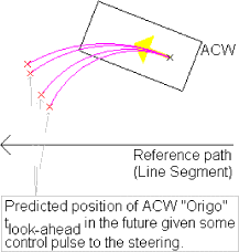
Figure A1 shows the principle. From the current state (box shown at an angle) the simulated positions are computed for various control pulses, and these predicted states are then evaluated with respect to
the “error” as described. This error function would take position, heading and steering angle (all relative to reference) into account.

Figure A1 Array of simulated positions as results of different changes of steering angle. The “error” of these positions relative to the reference path is then calculated and used to choose the
best change in setting.
1.2 Control pulse length sweep in Simulink
Figure A2 shows how the sweep across different pulses is performed in Simulink, as well as how the error function is invoked.
The input to the error function is the position relative to the reference line, the heading relative to the reference vector, the steering angle (relative to vehicle) and the vehicle speed. The speed is currently
ignored. Note that the position exchanged is the antenna position and not the Origo (rear wheel center) (since heading is also provided the Origo can be calculated from the Antenna position and vice versa).
Notes on computational complexity: the current approach has complexity O(N) where N is the number of possible control pulses to apply. Due to the short look-ahead time (compared to vehicle turn time) it
is expected that there will only be one “local minimum” for the error function. Thus the search could be improved to O(log N) or even better. With the current combination of On-Board Computer and
sample interval, the execution time is not a problem.
In case anyone are wondering why the HoldMinimum block does not have a reset input, this is because the iterated subsystem shown is encapsulated in an Enabled subsystem which is configured to start
“from scratch” whenever it is enabled.
1.3 The Error Function
The current error function (which is a rough first) defines optimum steering angle (relative to reference vector) and vehicle heading as a function of distance to reference line (and this function is configured
with the vehicle turn radius).
Figure A3 shows which steering angle (relative to reference) which is considered optimal. This is an arbitrary function. It does not take the turn speed (how fast the steering angle can be changed by the
steering actuator) into account.
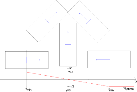
Figure A4 shows what is considered an optimal vehicle heading (this is related to the minimum turning radius, although it does not follow a “maximum-turn-approach” (where the optimal heading would be
arcos(1 – y/rmin)) – the gradient close to y=0 is less than it would have been if a “maximum turn” were used to model the optimum heading. Actually this makes the assumption of “instant change of steering angle” less critical). The function is identical to the steering angle function.
Click here to see Figure A2.

Figure A3 Steering angle considered optimal. Using the “bicycle” model for the vehicle, the optimal steering wheel angle can be derived from the steering wheel position. The figure shows steering wheels
with “optimal” direction for various position errors.

Figure A4 Heading considered optimal (i.e. for the vehicles sketched: given a position deviation, the heading shown, for each vehicle, is the one considered “optimal”)
The errors for steering angle and heading are then calculated as the deviation from these “optimal” values. When the vehicle heading is not way off, the total error is a weighted sum of the α, Ψ and y
contributions. The y-contribution is calculated according to figure A5.
The error contribution saturates, when position is more than minimum turn radius away from reference.

Figure A5 “Cross track error” cost contribution
Note that the simulation takes the actuator response time into account (as well as GPS delay), so another way to take the delays into account in the controller would be to increase the look-ahead time
beyond the controller sample time interval (1 s) plus the sum of delays. Thus the controller will perform a new simulation sufficiently early to set the steering angle to “anything” at the time the look-ahead time
“position” is reached. (Increasing the look-ahead time corresponds (in some respect) to lowering the “gain”).
1.4 LineServer
The previous sections described how a line is tracked. This section describes how the LineServer block takes a line segment from the route plan (Table A.2)and presents it to the tracking controller.
As seen in the screen dump (figure A6) the ImplementCode is taken from the P1 (the point travelled from) and the switch distance from P2 (the point travelled towards). i.e. when a point is reached, the
ImplementCode from this point becomes the new reference ImplementCode (i.e. the command to the implement controller). The switch distance tells when the point travelled towards is “reached” (Fig. 5.1).
When the point database is exhausted, the points are reused. The blocks P1_Server and P2_Server references the matrix 'routeplan' which should be set up by a “get_routeplan” script.
Click here to see Figure A6.
Table A2 Example of route plan points (one waypoint per line)
| 6121073.614 | 690178.452 | 1 | 1.900 |
| 6121077.509 | 690178.639 | 4 | 0.000 |
| 6121078.159 | 690178.670 | 4 | 0.000 |
| 6121079.817 | 690178.746 | 4 | 0.000 |
| 6121081.289 | 690178.794 | 4 | 0.000 |
The file is read using MATLABs DLMREAD function. The order of values is: Northing, Easting, ImplementCode and SwitchDistance. When the RelPos_x input is positive (corresponding to “vehicle” past
endpoint) the index into the matrix is updated (i.e. the next line segment is chosen). The relative distance of the vehicle to “switch line” should be calculated (outside this block) and fed to the input port
RelPos_x.
| Front page | | Contents | | Previous | | Next | | Top |
Version 1.0 November 2005, © Danish Environmental Protection Agency
|