Pesticides Research No. 114, 2007
Effects of Mechanical Weed Control in Spring Cereals – Flora, Fauna and Economy
Contents
- 2.1 Study sites and general design of the field study
- 2.2 Weeds and arthropods
- 2.3 Birds
- 2.4 Weed control
- 2.5 Statistical methods and modelling
5 Conclusions and Perspectives
Appendix A - Names of organisms studied
Appendix C - Statistical models
Appendix D - Data used for modelling plant–arthropod relationships
Preface
In a project 2004-2006 the effects of different intensities of weed harrowing on flora and fauna in agricultural fields were investigated on 6 large farms in eastern Denmark. The investigation is part of an array of pesticide research projects requested and financed by the Danish Ministry of Environment. The present project may been seen as interlinked with two previous projects, “Effects of reduced pesticide use on flora and fauna in agricultural fields” (Esbjerg & Petersen 2002) and “Flora and Fauna Changes During Conversion from Conventional to Organic Farming” (Navntoft et al. 2003). The three projects have the overall aim of elucidating the possibilities of reducing the use of pesticides and assessing the associated flora and fauna benefits. The first project demonstrated the benefits of 50-75% reduced dosages, while the second demonstrated the further effect of the conversion step to organic farming, i.e. without pesticides. From both these projects however, the question arose that the weed harrowing alternative to herbicides may also have adverse effects on flora and fauna, particularly if the frequency of harrowing is high. This question is dealt with in the present project, which furthermore includes analyses of the costs of various ways of improving the conditions for flora and fauna in agricultural fields.
The project requested a variety of expertises to be involved as appears from the below list of partners:
Project leader: Peter Esbjerg, Department of Ecology, Faculty of Life Sciences, University of Copenhagen
Botanical aspects: Department of Biology, University of Copehagen (Anne-Mette Jensen and Ib Johnsen)
Entomological aspects: Department of Ecology, Faculty of Life Sciences, University of Copenhagen (Søren Navntoft and Peter Esbjerg)
Ornithological aspects: Orbicon A/S (Bo Svenning Petersen)
Crop yield aspects: Danish Agricultural Advisory Service, The National Centre (Poul Henning Petersen)
Statistical aspects: Research unit on Statistics and Decision Analyses, Institute of Genetics and Biotechnology, Faculty of Agricultural Sciences, University of Aarhus (Kristian Kristensen)
Economic and weed control aspects: Institute of Food and Resource Economics, Faculty of Life Sciences, University of Copenhagen ( Jens Erik Ørum)
The practical execution of the project would not have been possible without the understanding and cooperation of the landowners, managers and others assisting in this project:
Asnæsgaard, Knud Eirik Viinsand
Oremandsgaard and Gl. Oremandsgaard Estate, Daniel Hage and the Manager Mogens Tved
Vibygaard Øst and Vibygaard Vest, Mogens Jørgensen and the Manager Christian Jørgensen
Viskingegaard, Niels Meinertsen
Others assisting in this project
Tonni Andersen
Anne Tulde Anttila
Niels Bruun
Nicolaj Correll
Martin Rasmussen Davidsen
Kaj Halberg
Tore Karlsson
Nina Karner
Christine Kastrup
Karen Kjeldsen
Jørn Lennart Larsen
Jan Martin
Bo Melander
Henrik Olsen
Steffen M. Thomsen
Furthermore thanks are due to the members of The Scientific Sparring Group:
Head of Research Unit Tommy Dalgaard (Faculty of Agricultural Sciences,Aarhus University)
M.Sc. Agronomy Lene Gravesen (Danish Environmental Protection Agency)
Special Advisor Jens Erik Jensen (Danish Agricultural Advisory Service, The National Centre)
Senior Scientist Mette Jensen (National Environmental Rersearch Institute, Aarhus University)
Senior Scientist Lise Nistrup Jørgensen (Faculty of Agricultural Sciences, Aarhus University)
Senior Scientist Pernille Kaltoft (National Environmental Rersearch Institute, Aarhus University)
Chairman and Special Advisor Jørn Kirkegaard (Danish Environmental Protection Agency)
M.Sc. Sociology Anne Mette Sørensen Langvad (Faculty of Agricultural Sciences, Aarhus University)
Technology and Science Director Niels Lindemark (Danish Crop Protection Association)
Senior Scientist Bent J. Nielsen (Faculty of Agricultural Sciences, Aarhus University)
Senior Scientist Niels Woetmann Nielsen (Danish Meteorological Institute)
Senior Scientist Egon Noe (Faculty of Agricultural Sciences, Aarhus University)
Senior Scientist Peter Odderskær (National Environmental Rersearch Institute, Aarhus University)
Professor Jørgen Eivind Olesen (Faculty of Agricultural Sciences, Aarhus University)
Senior Scientist Marianne B. Pedersen (National Environmental Rersearch Institute, Aarhus University)
Dr. Lise Samsøe-Petersen (Danish Environmental Protection Agency)
Associate Professor Jesper Rasmussen (Faculty of Life Sciences, University of Copenhagen)
Professor Peter Sandøe (Faculty of Life Sciences, University of Copenhagen)
Senior Scientist Chris Topping (National Environmental Rersearch Institute, Aarhus University)
Sammenfatning
Dette projekt er inspireret af to tidligere projekter og af et debatspørgsmål knyttet til økologisk dyrkning. Fra de to tidligere projekter, der anvendte mekanisk ukrudtsbekæmpelse som henholdsvis delvis og hel erstatning for herbicider, forelå indikationer af negative virkninger på jordlevende edderkopper og insekter samt virkninger på floraen, som rækker ud over det driftsmæssigt nødvendige. Disse forhold og spørgsmålet om den mekaniske ukrudtsbekæmpelses eventuelle skadevirkninger på lærkereder har dannet hypotesegrundlag for projektet, hvis formål har været at undersøge og kvantificere effekter af mekanisk bekæmpelse af ukrudt på flora og fauna. Dette skulle ses i lyset af muligheden for eventuelt at foreslå denne form for ukrudtsbekæmpelse som en af vejene til at nedsætte pesticidforbruget. Det har også været et mål at belyse de driftsmæssige omkostninger ved at opnå et givet niveau af flora og fauna i markerne.
Projektet er udført hos seks forsøgsværter, hvor effekterne af henholdsvis 2 tidlige striglinger og 2 tidlige plus 1 til 2 senere striglinger af ukrudt i vårhvede er sammenlignet, idet der er set på ukrudtsdække og artsammensætning, forekomst af nyttige edderkopper og løbebiller (som også er fugleføde) og ynglesucces hos sanglærke, vibe og strandskade. Et større datamateriale fra Dansk Landbrugsrådgivning har muliggjort modellering af udbytteeffekter af ukrudtsstrigling og herbicidanvendelse, og Danmarks Miljøundersøgelser har bidraget med supplerende data for ukrudtsstriglingers effekt på vibe- og strandskadereder.
Tre eller fire ukrudtsstriglinger reducerede ukrudtsforekomsterne markant sammenlignet med to striglinger; men der var ikke signifikant forskel på effekten af tre og fire striglinger. Ukrudtsbiomassen (tørvægt) blev reduceret med 43%, når antallet af behandlinger blev øget fra to til tre striglinger og med 48%, når antallet af striglinger blev øget fra to til fire. Biomassen af vårhvedeplanter blev 3% lavere ved en forøgelse af antallet af ukrudtsstriglinger fra to til tre og 6% lavere ved en forøgelse fra to til fire striglinger.
Øget ukrudtsstrigling medførte signifikant lavere tætheder af edderkopper af tæppespinder-familien ’Linyphiidae’ og af rovbillerne Tachyporus spp., men medførte ikke signifikant lavere tætheder af løbebillerne Agonum spp. og Bembidion spp. Tætheden af det samlede prædatorkompleks af de udvalgte prædatorer var 21-35% højere i parceller med kun to striglinger sammenlignet med parceller, som blev striglet yderligere to gange.
Der blev fundet en generel, positiv effekt af ukrudtsforekomst på leddyr, og den negative effekt af ukrudtsstrigling på leddyr kan delvis forklares som en indirekte effekt af nedsat ukrudtsbiomasse. 15-20 g ukrudtsbiomasse / m² (tørvægt) er nødvendig for at understøtte en høj tæthed af nyttedyr i maj-juni.
Der blev udført adfærdsforsøg med de to almindeligt forekommende løbebillearter Anchomenus dorsalis og Bembidion lampros. A. dorsalis viste præference for ustriglet jord mens B. lampros ikke havde præference for striglet eller ustriglet jord.
Ukrudtsstrigling havde en markant, negativ effekt på ungeproduktionen hos vibe og strandskade, hvorimod de negative effekter på sanglærkernes ynglesucces var moderate. Dette skyldtes primært, at yngletidspunktet hos vibe og strandskade var sammenfaldende med ukrudtsstriglingerne, mens størstedelen af lærkerederne først blev anlagt, efter striglingerne var afsluttet.
Kun 16% af lærkerederne blev udsat for strigling, men af disse gik hele 83% tabt. Den vigtigste årsag til redetab var ikke strigling, men prædation; en parameter, der også blev påvirket af antallet af striglinger. I parceller, der blev striglet to gange, var 65% af lærkerederne succesrige, mens dette kun var tilfældet for 28% af rederne i parceller, der blev striglet fire gange. Forskellen skyldtes dels, at det primært var 3. og 4. strigling, der ødelagde lærkereder, dels at prædationen var signifikant højere i parceller, der blev striglet fire gange. Det vurderes samlet, at striglinger udført højst 37 dage efter såning, og senest 20. maj, kun i ringe grad påvirker sanglærkernes ungeproduktion.
For vibernes vedkommende var ukrudtsstrigling den vigtigste årsag til redetab på forsøgsmarkerne: 40% af samtlige fundne reder blev ødelagt af strigling, og i yderligere 25% af rederne gik et eller flere æg tabt. Antallet af udklækkede unger per rede var 0,63, sammenlignet med 2,35 i ustriglede vårsædmarker og 2,80 på flerårige græsarealer. Som følge af vibernes tidlige ynglestart ramte også tidlige striglinger (og anden form for jordbehandling) et betydeligt antal vibereder. Succesrige omlæg er dog mulige, indtil afgrøden bliver for høj. Det vurderes, at alle striglinger og tromlinger, der foretages efter 1. maj, eller mere end nogle få dage efter kornets fremspiring, har en stærkt negativ effekt på vibens ynglesucces. Kun få strandskadereder blev fundet; men resultaterne tyder på, at strigling er mindst lige så skadelig for denne art som for viben.
Vårsæd er meget konkurrencestærke afgrøder, og ukrudtsbekæmpelse i veletableret vårsæd med et moderat ukrudtstryk (100-200 planter pr. m²) er derfor sjældent lønsom. For at undgå høstbesvær og opformering af ukrudt, som kan give problemer i efterfølgende afgrøder, tilstræbes der også i vårsæd med et moderat ukrudtstryk en relativ høj bekæmpelse (>70 %) af ukrudtet. Mekanisk ukrudtsbekæmpelse er tilsyneladende et effektivt alternativ til herbicider. En kemisk bekæmpelse med lave doseringer af herbicider giver imidlertid den økonomisk mest effektive ukrudtsbekæmpelse. Men også anvendelse af én tidlig strigling med høj intensitet (> 20% jorddækning af afgrøden) er en økonomisk attraktiv mulighed, idet der kun er 0,7 hkg/ha mindre gennemsnitligt merudbytte end ved den bedste kemiske løsning. For planteavlere, som ønsker at begrænse deres pesticidforbrug, er en endnu lavere herbiciddosering en mulighed, der i tilfælde af utilstrækkelig effekt kan følges op med en strigling. Dog skal denne strigling være tidlig for at undgå skader på lærkereder, og af hensyn til lærker og biodiversitet må denne blandede (men i øvrigt meget effektive) fremgangsmåde frarådes. Modelberegninger har vist, at det vil koste mindre end 20-25 DKK pr. ha at tillade en ukrudtsbestand, der kan bidrage til at skabe grundlag for en højere tæthed af arthropoder.
Af projektets resultater kan konkluderes, at et behersket bunddække af vilde planter/ukrudt er til gavn for smådyr og fugle, og dette kan opnås på forsvarlig vis med behersket strigling (maks. 2 gange). Løsninger med mere end 2 striglinger er bekostelige og skader både insekter og fugle unødigt. Tidspunktet for strigling er kritisk for jordrugende fugle. Skaden på lærkereder er begrænset, hvis der senest strigles 35-37 dage efter såning og aldrig efter 20. maj. Overholdes disse tidsrammer er der intet grundlag for at anse økologisk dyrkning og mekanisk ukrudtsbekæmpelse i vårsæd som en trussel for lærkebestanden. I det bredere perspektiv kan mekanisk ukrudtsbekæmpelse, i betragtning af den ringe meromkostning, anses for et rimeligt forslag til nedbringelse af bedrifters pesticidforbrug. Om det også er et godt tiltag for at forbedre agerlandets biodiversitet er et åbent spørgsmål. Marker med mange ynglende viber er endvidere en klar undtagelse, idet denne arts tidlige redeetablering gør den yderst sårbar for strigling, hvorfor særlige beskyttelsesforanstaltninger for sådanne arealer bør overvejes. Disse arealer bør heller ikke udsættes for herbicider og insekticider, da fødemængderne, og dermed vibeungernes overlevelse, så reduceres væsentligt.
Summary
The present project has a background in two earlier projects and in a standing debate about weed harrowing as part of organic farming. The first project partly used weed harrowing in a row crop while the second on effects of conversion to organic practice fully used weed harrowing. Results of both indicated that more than two weed harrowings might negatively influence wild flora more than economically necessary, and also damaged arthropods. These results, and the often postulated damage to nests of ground-dwelling birds, were turned into hypotheses.
In accordance with these hypotheses, the aim of the project was to investigate and quantify effects of weed harrowing on flora and fauna in the light of the potential of this weeding methodology as part of the approaches towards a reduced use of pesticides. A further aim was to calculate/model costs of particular practices directed towards improvement of flora and fauna in fields.
The project included six host farms on which we studied the effects of two or four times harrowing in spring sown wheat on weed cover and diversity, densities of selected spiders and beetles (agriculturally beneficial predators which are also bird food) and breeding success of Skylark, Lapwing and Oystercatcher. A large set of data from the Danish Agricultural Advisory Service made the modelling of yield effects possible, and the National Environmental Research Institute supplied additional data on breeding success of Lapwing and Oystercatcher in weed harrowed fields.
A marked reduction in weed occurrence was seen when the number of weed harrowings was increased from two to three or four. No significant change, however, in weed occurrence was found when harrowing frequency was increased from three to four weed harrowings. The weed biomass was reduced by 43% when the weed harrowing was increased from two to three times, and by 48% at an increase from two to four times harrowing. The crop biomass was reduced by 3% when the number of weed harrowings was increased from two to three, and by 6% at an increase from two to four times harrowing.
Weed harrowing had a significant negative effect on densities of the spiders Linyphiidae and the rove beetles Tachyporus spp., but not on the carabids Agonum spp. and Bembidion spp. Densities of the common arthropod predator complex were significantly higher (21-35%) in the plots subject to only two harrowings when compared with the adjacent plots subject to two additional harrowings.
A general positive relationship was found between weed biomass and predator densities, and the negative effect of weed harrowing could partly be explained as an indirect effect of lower weed biomass. 15-20 g weed biomass / m² (dry mass) is necessary to support a high density of beneficials in late May – early June.
Choice-experiments with two common carabid species revealed that Anchomenus dorsalis preferred un-harrowed soil whereas Bembidion lampros had no preference for harrowed or un-harrowed soil.
Weed harrowing had a strong, negative effect on the breeding success of Lapwings and Oystercatchers, while only a modest number of Skylark nests were damaged. The main reason for this was that breeding in Lapwing and Oystercatcher coincided with the weed harrowings, whereas most Skylark nests were established later.
Only 16% of the Skylark nests were exposed to weed harrowing, but 83% of these nests were destroyed. Predation was the main cause of nest failure, and predation risk was also affected by weed harrowing. In plots that were subject to two harrowings, 65% of the Skylark nests were successful, whereas this was the case in only 28% of the nests placed in plots where four harrowings occurred. There were two reasons for this difference: few Skylark nests were active during the first two weed harrowings and predation rates were significantly higher in plots with four times harrowing. It is concluded that weed harrowing performed no more than 37 days after sowing and no later than 20 May has only minor effects on Skylark breeding success.
For the Lapwing, weed harrowing was the most frequent cause of nest failure. On fields where weed harrowing was carried out, 40% of all Lapwing nests were completely destroyed and in a further 25% one or more eggs were lost. The mean number of hatchlings per nest was 0.63 in fields with weed harrowing, compared to 2.35 in similar fields where weed harrowing was not performed and 2.80 in perennial grassland. Because the breeding activities normally begin in April, even early weed harrowings (and other soil treatments) destroy a sizable number of Lapwing nests. Successful re-laying is only possible until shortly after crop emergence. It is concluded that weed harrowing (and rolling) performed after around 1 May, or later than a few days after crop emergence, has a strong, negative effect on Lapwing breeding success. Few Oystercatcher nests were found, but the available data suggest that weed harrowing is at least as damaging to this species.
Spring cereals are very competitive to weeds, and chemical as well as mechanical weed control often results in a negative net yield gain in these crops. To avoid harvest problems and long-run dynamic problems in the following crops the weed is however, controlled (>70% reduction in weed biomass) in spring cereals as well. Mechanical weed control appears to be an effective alternative to herbicide use, but the analyses indicate that the economically most efficient strategy is the use of a low (but still effective) dosage of herbicide. However, the weed control effect of an early, single, and intensive (>20% soil coverage of the crop) post-emergence harrowing is also very satisfactory, the only drawback being the 0.7 hkg/ha higher net cost than the low dosage herbicide treatment. For farmers with reduction of herbicide input as an aim it may be cost effective to apply a low dosage and, in case of insufficient control, follow up with harrowing. This has, however, to be done early to be efficient and to avoid damage to Skylark nests, and from a biodiversity point of view the mixed strategy cannot be recommended. Modelling has shown that the weed population needed to sustain a high density of arthropods may be allowed at a cost below 3€ per ha.
From the project results it is concluded that a certain weed cover is beneficial to insects and birds and such a weed cover may be a positive result of a harrowing which is not too intensive. By contrast, more than two times weed harrowing is damaging to plants, insects and birds and is not economically justified. The timing of harrowing is crucial to ground-nesting birds. If performed no later than 35-37 days after sowing, and never after 20 May, weed harrowing has only minor effects on Skylark breeding success. With this observed, there is no reason to accuse mechanical weeding of being damaging to Skylarks. Due to the very limited extra cost, weed harrowing might also be considered one of the tools for reducing pesticide use in other farm practices. The biodiversity effects of weed harrowing versus reduced herbicide dosages are unclear. The only clear exception to this is areas with high numbers of breeding Lapwing. This species is highly vulnerable to even early harrowings, and special protection measures for such areas should be considered. These measures should also include the omitting of herbicides and insecticides, to ensure sufficient amounts of food items and thus improve hatchling survival.
1 Introduction
1.1 Background
In the context of protecting biodiversity in modern intensive agriculture, pesticide use is a focus area which in Denmark has been treated by the Bichel Commission (1999). This Commision recommended several approaches to reducing the use of pesticides and since that time a number of research projects have been carried out, mainly financed by The Danish Ministry of Environment. Organic farmland was already known to hold a higher diversity of plants, insects and birds than conventionally farmed areas (Braae et al. 1988, Hald & Reddersen 1990), and accordingly the Bichel Commission recommended that a higher proportion of Danish farmland should be farmed organically, because a promotion of this practice may act as one of the approaches towards the general goal of reducing the use of pesticides.
Within research, particular attention was also paid to organic farming and its methods. However, there was very little knowledge about the immediate effects of a switch of farming practice in contrast to the much broader information about the status after five or more years of organic practice.
Weeds are major constraints to crop production (Marshall et al. 2002), and as a consequence weed control is an almost universal farm operation. On one side, weed control through herbicide use accounts for a major part of the Danish pesticide consumption, and on the other side, mechanical weed control is well established in organic farming (Rasmussen et al. 1997). Mechanical weed control therefore called for particular interest. Furthermore, an earlier project on effects of reduced of pesticide use, accomplished through a reduction of dosage per hectare, partly included mechanical weed control, which proved fairly efficient but did also leave a slight question on possible side effects on ground dwelling predators (Esbjerg & Petersen 2002). A follow-up project dealing with the conversion phase from conventional to organic farming (Navntoft et al 2003) supported the need for further investigation of effects of intensive mechanical weeding on non-target organisms. In that project it was found that arthropods living above the ground, mostly on plants, were unaffected or increased after the conversion to organic practice while the abundance of arthropods on the soil surface was reduced. Thus there were positive biodiversity effects already the first year after conversion, but also rather clear indications of negative effects on a part of the fauna on the soil surface.
Other studies have demonstrated that mechanical weed control has direct, negative effects on beneficial, epigaeical arthropods. Mechanical crop treatments generally reduce the numbers of polyphagous predators directly, e.g. through mechanical damage, and indirectly through habitat disturbance (Thorbæk & Bilde 2004). Specifically for weed harrowing, Thorbæk & Bilde (2004) found a significant direct negative effect on spiders but no significant effects on carabids or staphylinids, neither directly nor indirectly.
Efficient weed and pest control, whether mechanical or chemical, affects populations of farmland birds negatively by reducing the amount of available food, such as weed seeds and arthropods (e.g. Potts 1986, Boatman et al. 2004). Furthermore, it is widely believed that mechanical weed control destroys sizable numbers of nests of bird species such as Skylark Alauda arvensis and Lapwing Vanellus vanellus that breed in the fields. The evidence of an effect on Skylark nests was until recently largely anecdotal, but a recent project (Odderskær et al. 2006) demonstrated that between 50 and 100 % of the nests that were exposed to weed harrowing were destroyed. However, the impact on the Skylark population was negligible because very few nests were active at the time when weed harrowing is normally carried out. By contrast, the negative effects of farming operations on Lapwing breeding success are well documented (e.g. Galbraith 1988, Shrubb 1990, Berg et al. 1992) and may have serious effects. The Danish population of Lapwing was reduced by approximately two thirds from 1976 to 2004 (Heldbjerg 2005), and Lapwing populations all over Europe have plummeted since 1990, to such an extent that the species is now considered Vulnerable according to IUCN Red List criteria (BirdLife International 2004). The available demographic data indicate that the main reason for this decline is an insufficient production of fledglings (Petersen submitted).
Following up on the work of the Bichel Commission, Ørum (2004a) found that a so-called Skylark-friendly farming practice might be implemented at a cost of 10 to 25 DKK per ha. This farming practice did not include mechanical weed control. Ørum (2004) further demonstrated that a general reduction of pesticide use, accomplished through taxes or quotas, would not by itself lead to a more Skylark-friendly practice; implementation of such practices would always require special attention.
Farmers are basically looking for weed control strategies that effectively control the weeds and cause as little damage to the crop as possible. Mechanical weed control may be one efficient strategy to consider. According to the Danish Agricultural Advisory Service (Petersen 2002) weeds can effectively be controlled by using weed harrowing in spring barley, but the mechanical weed control is in general more expensive (around 0.5 hkg per ha) than the most efficient low-dose herbicide strategies.
The present project aims at quantifying the effects – positive or negative – of weed harrowing on selected flora and fauna elements and also at elucidating the efficiency issue. Naturally, the focus is on organic farms where mechanical weed control is the sole option and is often used very systematically, sometimes at high frequency, i.e. up to 4-5 annual treatments (or even more in row crops such as maize). However, the efficiency (profitability and weed control effect) of supplementing or substituting chemical weed control by weed harrowing in conventional farming is also considered, mainly with the purpose of estimating the costs of a potential adoption of more biodiversity-friendly weed control strategies. This aspect is necessary if further suggestions for protection of biodiversity shall be considered.
1.2 Aim and conditions
The present project has two main aims:
1) to investigate and quantify the effects of mechanical weed control on flora and fauna in order to elucidate the significance of this deweeding methodology when it interacts with other IPM components and the focus is promotion of natural elements through diminished use of pesticides.
2) to calculate/ model the costs of particular practices necessary to obtrain particular improvements of flora and fauna.
These two aims are interconnected to several hypotheses and some presumptions.
Hypotheses
That intensive mechanical weed control:
1) Causes floral damages at a level which raises questions about the balance between flora damage and agricultural benefit.
2) Causes density reduction of the epigaeic insects which are both agriculturally benefial and important as bird food.
Presumptions
a) The anticipated biological results will be so well related to the results of preceding projects (Esbjerg & Petersen, 2002, Navntoft et al. 2003) that the costs at farm level of improved natural elements (farmers expense of a certain number plus one extra of wild flowers, insects and Skylarks on a particular area) can be calculated.
b) That the results can be used in a broader context – the results on effects of mechanical weed control can be extrapolated to other types of agricultural practice.
2 Methods
- 2.1 Study sites and general design of the field study
- 2.2 Weeds and arthropods
- 2.3 Birds
- 2.4 Weed control
- 2.5 Statistical methods and modelling
2.1 Study sites and general design of the field study
The study was carried out in 2004 and 2005 in organic fields that were spring-sown with wheat (Triticum aestivum L.). In both years, six farms located on Zealand, Denmark (Figure 2.1) were used for the study. Two of the farms (Asnæsgård and Viskingegård) were located on Northwestern Zealand, Denmark, another two (Vibygård SØ, Vibygård NV) on Eastern Zealand and the remaining two farms (Oremandsgård and Gl. Oremandsgård) were located on Southeastern Zealand (Figure 2.1, Table 2.1). All study farms were situated on rather clayish soils, which are common in most of Eastern Denmark.
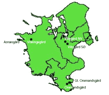
Figure 2.1. Mapped locations of the six study farms in Zealand in Denmark.
A spring-sown crop as selected as the experimental crop because spring-sown cereals are the crops favoured by one of the main study species, the Skylark Alauda arvensis. Spring-sown wheat was preferred to barley and other spring crops because the current trend in Danish organic farming is towards wheat.
In both years the six host farms contributed one field each, yielding a total of 12 experimental fields. In each field, two adjacent plots of approximately equal size (preferably 6 ha and rectangular, in practice 5 to 8 ha and of varying shape) were demarcated, thus retaining the same basic design as in previous studies (Esbjerg & Petersen 2002, Navntoft et al. 2003). This plot size made it probable that a sufficient number of Skylark nests could be found. All plots were placed some distance away from hedgerows and coverts, in an attempt to ensure equal risk of nest predation across plots (within each field).
In each field, the two plots were randomly allocated to one of two different treatments: 2 weed harrowings and 4 weed harrowings. At each farm, the first two harrowings were performed on the same days in “2 harrowings” and “4 harrowings” plots. The first harrowing was carried out before or coinciding with the emergence of the wheat, while the second harrowing was carried out after crop emergence. After that, “4 harrowings” plots were harrowed two times more while “2 harrowings” plots were left untreated. The timing of weed harrowing and other farming operations was the individual farmer’s decision (Table 2.1). The growth stage intervals for the timing of the four weed harrowings were 09, 12-22, 13-31 and 22-46, respectively (decimal code by Tottman & Broad 1987). No restrictions were placed on the farmer with respect to cultivation of the experimental fields before the experiments, previous crop, wheat variety, sowing date, fertilizer use etc.
Table 2.1. The location of the experimental farms and timing of sowing and harrowing.
| Farm | Co-ordinates | Sowing | Weed harrowing | ||||||||||||
| (wgs84) | First | Second | Third | Fourth | |||||||||||
| 04 | 05 | 04 | 05 | 04 | 05 | 04 | 05 | 04 | 05 | ||||||
| Asnæsgård | 55° 39' 48" N; 10° 57' 18" E |
12/4 | 3/4 | 21/4 | 20/4 | 28/4 | 6/5 | 10/5 | 20/5 | 19/5 | 30/5 | ||||
| Viskingegård | 55° 39' 30" N; 11° 14' 42" E |
12/4 | 16/4 | 19/4 | 22/4 | 24/4 | 5/5 | 11/5 | 18/5 | 30/5 | 9/6 | ||||
| Vibygård SØ* | 55° 33' 46" N; 12° 01' 22" E |
13/4 | 3/4 | 21/4 | 18/4 | 12/5 | 13/5 | 28/5 | 26/5 | 8/6 | 10/6 | ||||
| Vibygård NV* | 55° 33' 46" N; 12° 01' 22" E |
15/4 | 4/4 | 23/4 | 18/4 | 14/5 | 14/5 | 1/6 | 20/5 | 8/6 | 26/5 | ||||
| Oremandsgård | 55° 04' 10" N; 12° 03' 53" E |
17/4 | 12/4 | 22/4 | 25/4 | 11/5 | 17/5 | 18/5 | 25/5 | 26/5 | 9/6 | ||||
| Gl. Oremandsgård | 55° 04' 47" N; 12° 06' 18" E |
18/4 | 13/4 | 22/4 | 25/4 | 11/5 | 13/5 | 18/5 | 19/5 | 26/5 | 25/5 | ||||
*Distinct parts of the same holding; co-ordinates denote location of main building
Additional ornithological studies were carried out in a number of fields at one of the farms (Vibygård) in 2006. The crops involved and the farming operations carried out are described in section 2.3.2 below.
2.2 Weeds and arthropods
2.2.1 Field study
Sampling was restricted to the main crop area. Plot margins of minimum 20 m from the field edge were excluded in order to minimise interference between plots and field edges. Within each plot, 11 subplots of 100 m² were selected for sampling (Figure 2.2). For each subplot, the distance to the nearest field margin or other perennial vegetation was measured using GPS. The 11 sub-plots were distributed evenly along the tramlines where the sampling equipment was transported in order to reduce crop damage. Each sample from a subplot comprised four subsamples of 0.15 m² circles. Within subplot no 11, five subsamples were collected. In total 45 = 10´4 + 5 subsamples were collected per plot.
Effects of weed harrowing were determined by estimating arthropod abundances and vegetation biomass simultaneously in the plots subject to two and four times weed harrowing, respectively. Sampling was carried out within one week after the second, the third and the fourth mechanical weed harrowing.
The soil flooding method was used to obtain density estimates of each species of arthropods. The method is described by Brenøe (1987) and Basedow et al. (1988). A 25 cm high circular tube with cross section 0.15 m² (equals one sub sample) was quickly inserted approximately 10 cm into the soil. The above ground vegetation was immediately harvested by cutting and separated into four plant biomass groups: wheat, undersown crop, perennial weed species and annual weed species. While cutting the vegetation all visible arthropods were collected and transferred to 70% alcohol. Immediately after the vegetation was collected the tube was filled with water (approximately 5 l) and all emerging arthropods were collected from the surface. Another 5 l of water was added and the upper soil layer and water was mixed and stirred in order to extract remaining arthropods.
In 2004 the soil flooding method was supplemented with pin point analyses to estimate vegetation cover and pitfall trapping to sample epigaeic arthropod predators. It was decided to use two sampling methods in order to clarify which one was the most efficient and therefore should be the final choice.
Pin point analysis was done with a 1 ´ 1 m² frame equipped with a 10 cm thread mesh, giving 100 intersection points. At each point, a 3 mm Ø pin was inserted vertically, and the plant hit was recorded. The pin point frequency in percent equals number of hits per frame (0-100). The pin point frequency is correlated with cover. One frame per each of the 11 subplots was analyzed. The pin-point analyses were done shortly after 2nd and 4th harrowing in all fields, and only 2004.
Pitfall trapping was carried out using 20 pitfalls placed within each plot as presented in Figure 2.2. The traps were placed approximately 1.5 m from the soil flooding spots. Each trap consisted of a plastic container (diameter 92 mm, depth 80 mm) partly filled with 200 ml of trapping and preservation fluid (a mixture of 1:1 ethylene glycol and tap water, with one drop of nonperfumed detergent per 10 l). A flat roof (20 cm x 20 cm) was placed 15 cm above each of the pitfalls to protect them from rainfall and from predation from birds. The traps were put in the field within a few days after the 2nd, 3rd and 4th weed harrowing and within three to seven days thereafter the traps were collected, labelled and placed in a cold storage until sorting.
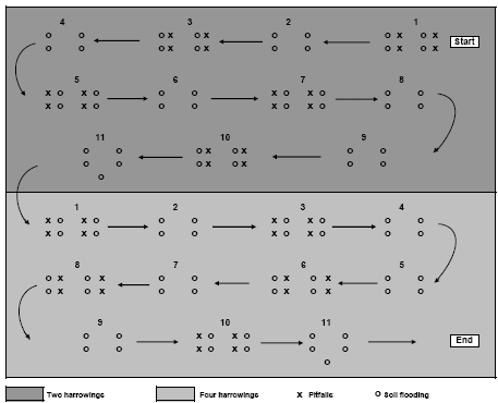
Figure 2.2. Schematic diagram of the sampling design in a single experimental field. Pitfall sampling was carried out in 2004 only. Each plot was minimum 6 ha. Arrows indicate tramlines.
In the laboratory, the vegetation samples were dried at 80oC for at least 48 hours, kept at 18-20 oC and weighed. The arthropods were identified under binocular microscope at 5 - 40 x magnification. Araneae were identified at minimum to family following Roberts (1985-1993, 1995). Carabidae were identified to species following Lindroth (1985, 1986) and Staphylinidae were identified to sub-family or more detailed level following Hansen (1951, 1952, 1954). Other arthropods were identified at minimum to order. The scientific, English and Danish names of the organisms studied are presented in Appendix A.
Loooking at the individual weed species the occurring weed species in one the 0.15 m² circles (subsamples) was cut off at soil level and the above-ground biomass of each species was transferred to separate paper bags to determine the dry biomass for each species. The biomass in g dry matter of each species pr subsample was weighed after two, three and four times weed harrowing respectively as describes previously. In total, 81 sampling units were used, of which 65 were determined to species level. In some cases, only genus level determination was possible. Taxonomy according to Hansen (1981).
In august 2004 and 2005 weed phenology was studied. The flowering and diversity of weed species was investigated in 10 of the 11 subplots for each treatment. At each subplot the occurring weed plants, in 2 squares at 0.25 m² each, were determined and classified into one of the following growthstages: seedlings (seed leaves present and less than 5 leaves developed), vegetative plants (no seed leaves present and no flower bud, flower or seed present on the plant), flowering plants (flower bud, flower or immature seeds present) and seedsetting plants (plant with mature seeds or plant that has dropped the seeds).
Species diversity for the weed flora is given by species density (number of species at a given area).
Frequency of flowering is the number of flowering or seed setting weed plants in a square divided by the total number of weed plants in the square.
2.2.2 Field arena experiments
Choice-experiments with carabids placed within steel frames in the field were carried out in order to investigate the indirect effects of weed harrowing measured as the animals preference for weeded and un-weeded ground. The field arena experiments were selected for the reason that results were closer to natural conditions than laboratory experiments as the field provides natural light, humidity and soil conditions, hiding places and natural plant canopy. It was investigated whether the two carabid species Anchomenus dorsalis (Pontoppidan) (subgenus under the genus Agonum) and Bembidion lampros (Herbst) preferred weed harrowed or non-harrowed field.
The experiments were carried out in 2006 and located within a 4 ha South-Eastern corner of a 43 ha large field on Vibygård SØ (Figure 2.3). Against East the experimental area was bordered by a road with a 5 m grass verge in between. Against South the field was bordered by a 20 m wide set-aside area covered with grass and various herbs. The soil was sandy-clay and the crop was spring wheat (cv. Fiorina sown 14 April). Just prior to crop emergence 23 April, the entire field was weed harrowed. Another weed harrowing was carried out 26 May but this time the harrowing excluded the 24 m wide headland.
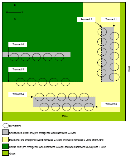
Figure 2.3. Illustration of the field arena experiments in the South-Eastern corner of an organic spring wheat field. The area was approximately 200 ´ 200 m². Two experiments were carried out, one from 3 - 5 June and one from 9 - 11 June. For the first experiment transects 1, 2, 4 and 5 were used and for the second experiments, transects 3, 4 and 6 were used. The steel frames were placed in such a way that the transects separated the area within the frames in halves with undisturbed soil and vegetation in one half and newly weed harrowed soil in the other half. For each experiment 100 frames were used.
The field arena experiment was carried out twice; the first time from the 3 - 5 June and then again from 9-11 June. At this time the crop was 30 – 40 cm high and GS 32 - 33 (Tottman and Broad 1987).
3 June the headland within the experimental area was weed harrowed, however in such a way that a 2 m wide strip of the headland was left un-harrowed (Figure 2.3). This strip was created by lifting one of middle sections of the harrow (Einbock Aerostar®, 24 m wide harrow from 2002) during operation. The weed harrowing was carried out on slightly humid soil at 7 km/hr and at a pressure of 60 bar, leaving lines with fairly sharp boarders between the weeded an un-weeded soil (four transects).
The steel frames themselves (diam 43 cm, ht 10 cm) caused some shading within the arenas, especially when the sun was at a low angle on the horizon, which could affect the behaviour of the beetles. Different orientations of the transects and the different orientation of weeded and un-weeded soil between transects, secured randomly light intensity between weeded and un-harrowed parts within the arenas, thereby avoiding the introduction of systematic errors in the experimental design.Two of the transects (no. 1 and 2) were running North - South and two were running East – West no. 3 and 4) (Figure 2.3).
4 June, 100 frames were evenly distributed along the transects and placed in such a way, that one half of each arena was covering the weed harrowed field and the other half was covering undisturbed ground. Transect 3 however, had such a poor quality that we considered it unusable for the experiment due to little differences between the weed harrowed and un-harrowed fields. This was caused by unevenness of the ground being an obstacle of efficient weed harrowing. Instead another transect (no. 5) was chosen for the experiment (Figure 2.3). This transect was created by the outer section of harrow.
Not all parts of a transect used were suitable for the choice experiments. Consequently the frames were put in spots selected with the criteria that the harrow had created a clear difference between harrowed and un-harrowed field with a relatively sharp boarder. The frames were forced 5 – 6 cm into the soil leaving 4 - 5 cm above the soil level. On the inside of each arena the upper 5 cm was covered by smooth tape (tesa®) in order to prevent beetles from escaping.
After the establishment of the frames in the field 5 June, each arena was gently searched for naturally occurring beetles, which were removed. Following that, one A. dorsalis and one B. lampros was put in the middle of each arena between 4.30 and 5.30 p.m. The beetles had been marked the previous day with pink fluorescent powder (product from Sun Chemicals A/S), making it possible to trace the beetles in darkness and to distinguish the experimental beetles from possible naturally occurring individuals. The experimental beetles were collected in various organic fields in Eastern Zealand between 24 April and 16 May, using aspirators or pitfalls, which were emptied on daily basis. The beetles were kept in polyethylene boxes (22 x 17 x 6 cm³) with a bottom of slightly humid sand and stored in a refrigerator without food and light at 5°C until use.
Between 11 pm and 0.30 am the beetles were traced within the arenas with as little disturbance as possible using UV-lamps (UNIROSS Lightpower CH8858) and their position recorded (weeded or un-weeded location) (Figure 2.4).
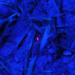
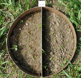
Figure 2.4. Left picture: night photo of an A. dorsalis marked with fluorescent powder and exposed to UV-light. Right picture: steel frame no. 67, 5. June. Undisturbed soil is to the left and weed harrowed soil to the right.
The following day (5 June between 8 am and 10 pm) the position of the beetles within the arenas were recorded again in random order using the following procedure: first a 43 cm x 10 cm steel plate was forced into the ground within the arena, thereby separating the frame in a weeded and an un-weeded half (Figure 2.4). The plate prevented movements of the beetles from one half to the other during inspection. After a brief search for beetles the vegetation from each half was excised at ground level and collected. The biomasses from the weeded and un-weeded halfs were kept apart, separated into weeds and crop and put in paper bags for later biomass estimation using the same procedure as described for the field experiment. Simultaneously with this operation all B. lampros and A. dorsalis seen were collected. Thereafter the upper soil layer was searched for beetles. If the beetles could still not be found, water was added to the arena in order to extract remaining beetles as described for the field experiment (section 2.2.1). All beetles looking like the two experimental species were collected, numbered and their position was recorded together with the name of the finder and the time they were found. They were placed individually in small labelled polyethylene chambers and brought to the laboratory for further species identification and for tracing the marked beetles.
The weather from 3 - 5 June was unstable ranging from dry and sunny to windy with a few showers. The temperatures were 10-20°C. Due to the unstable weather conditions, which were anticipated to have a strong influence on the beetle behaviour, it was decided to repeat the experiment the following week.
9 June a new weed harrowing was carried out, which extended the transects 3 and 4 against West and created a new transect (no. 6) along a gap which had been left untouched by the previous weed harrowing 26 May (Figure 2.3). An attempt was made to harrow transects 1 and 2 again, but we found the result unsuitable for the experiment. The soil was dry and it was weeded with a speed of 10 km/h and at a pressure of 100 - 125 bar. 10 June the 100 frames were placed on transects 3, 4 and 6 on appropriate positions which had not been used before, and following the procedure described previously. No attempt was made to remove naturally occurring beetles from within the frames. Following that, one A. dorsalis was put in the centre of each arena between 2 – 3 pm. The beetles were not marked with fluorescent powder because night observations were omitted from the experiment and because of the risk that it would affect beetle behaviour inappropriately. Furthermore it was decided to include naturally occurring beetles in the experiment. No B. lampros was put artificially as we decided to rely on naturally occurring beetles based on the experience from the earlier study. The vegetation was harvested roughly within the arenas to enhance the chance of finding the beetles but no attempt was made to collect and quantify it because it would become too time consuming. On 11 June between 9.30 am and 10 pm the position of the beetles (harrowed or non-harrowed ground) were recorded as described previously, with the exceptions that this time the arenas were sampled in chronological order to save time and that all arenas were floated to make the experimental condition more uniformly.
The weather from 9 - 11 June was stable with sunshine and light wind. 9 June the day temperature ranged from 15-20°C. 10 and 11 June the day temperatures were between 20-25°C.
2.3 Birds
2.3.1 Skylark
On all experimental fields, nests were searched in 2004 and 2005. The search for Skylark nests on a field began a few days after emergence of the crop, i.e. between 26 April and 4 May (or 13 to 23 days after the field was sown), when the tramlines were just discernible.
Following the recommendations of Odderskær et al. (1997), nest searches were performed using a 4WD vehicle as a hide. While driving up and down the tramlines at low speed (10-15 km/h), the driver and a co-observer constantly looked out for Skylarks. The distance between tramlines varied between fields (12, 18 or 24 m), depending on the equipment used. Whenever a lark was seen rising from the field within 10-20 m of the vehicle, the area from where the bird was flushed was searched by the observers. Also, if a Skylark was seen carrying food or nest material in its bill or showing other signs of nesting behaviour, the car was stopped and the bird was followed using binoculars. At each visit the field was driven through twice, in opposite directions.
As soon as a Skylark nest was found, its location was recorded using GPS
and the site was (in 2004) also marked with two sticks placed c. 5 and 10 m from the nest. This way of marking was used to avoid attracting predators to the nest. However, the nests sometimes proved difficult to re-locate for the observers if the weed cover was dense, increasing search time and vegetation trampling and thus perhaps increasing the risk of predation. Therefore, in 2005 two more sticks (placed so that the two rows of sticks intersected each other at the nest) were used to mark each nest. As there were many other sticks placed in the experimental fields (cf. section 2.2.1), we believe that the marking of nest locations did not attract predators to the nests.
Each field was visited at 4 to 5 day intervals and, in addition to this, after each weed harrowing. At each visit to a nest, its stage was recorded (nest cup without/with complete lining, eggs, young) and the number of eggs and young (alive/dead) in the nest was noted. Age of nestlings was estimated from their size and plumage development. In cases where the age of the young was known (because the nest was visited at time of hatching) it was possible to calibrate our estimation of nestling age at later visits. We believe from these calibrations that our estimations of age, and thus of the day of hatching, were accurate ± 1 day.
Skylark eggs are laid at the rate of one per day, usually early in the morning (Donald 2004). If a nest was found with an incomplete clutch, the date of laying of the 1st egg was therefore known exactly. Also, if a nest was found during nest-building but contained eggs at the next visit, the date of 1st egg could usually be accurately estimated. Incubation generally begins with the laying of the last egg (Cramp 1988, Donald 2004) and the normal incubation time is 11 days (Cramp 1988), although it may vary between 10 and 13 days (Donald 2004). Based on these figures and on the estimations of nestling age, date of 1st egg and start of incubation were estimated in those cases where a nest was discovered with a complete clutch (usually 3 to 5 eggs) or with nestlings.
The young leave the nest while still flightless, usually at an age of 8-10 days (Cramp 1988). Nests containing live young at the last visit before day 8 after hatching and found empty at the next visit (day 8 or later) were classified as successful unless there were clear signs of predation (such as scraped out nest material) or other causes of nest failure. In case of nest failure, the cause was noted (predated, destroyed by weed harrowing, flooded, abandoned etc.). No attempts were made to estimate the survival of chicks after they had left the nest.
The number of visits to each field is shown in Table 2.2. In 2004, the last nest searches were performed on 26 June, with later visits being restricted to controls of previously found nests. In 2005, nests searches continued until 21 July (with later controls of nests), allowing second broods to be included. The stopping of the nest searches in July 2005 coincided with a clear decline in Skylark activity on the fields.
Table 2.2. The number and timing of field visits with searches or controls of Skylark nests in 2004 and 2005.
| Farm | 2004 | 2005 | ||
| Period | No. of visits | Period | No. of visits | |
| Asnæsgård | 29.04 – 25.06 | 12 | 02.05 – 20.07 2) | 19 2) |
| Gl. Oremandsgård | 04.05 – 22.06 | 8 1) | 03.05 – 17.07 | 16 |
| Oremandsgård | 04.05 – 07.07 | 15 | 04.05 – 21.07 | 18 |
| Vibygård NV | 28.04 – 28.06 | 18 | 26.04 – 31.07 | 23 |
| Vibygård SØ | 28.04 – 10.07 | 18 | 26.04 – 23.07 | 22 |
| Viskingegård | 29.04 – 30.06 | 12 | 02.05 – 20.07 | 18 |
1) Number of visits reduced because no signs of Skylark breeding were observed
2) A change of study field was rendered necessary on 17 May (after 4 visits) due to a mistake in the experimental harrowings
The variation between fields in tramline distance (12, 18 or 24 m) possibly affected the probability of nest detection. However, tramline distance and number of visits did not vary between plots within a field. Therefore, the number of nests and the estimates of nest success rate are comparable between treatments, but not between fields or years.
2.3.2 Lapwing and Oystercatcher
In 2004, two of the experimental fields (Oremandsgård and Vibygård NV) held breeding Lapwing (at least 6 and 5 pairs, respectively). Because Lapwing nests were also supposed to be vulnerable to mechanical weed control, and the incubating birds were fairly easily seen in the low vegetation, it was decided to include the species in the study. Thus, Lapwing nests were recorded and marked in the same way as the Skylark nests.
In 2005, searches for Lapwing nests were included from the outset and were also performed (by scanning the fields with binoculars) at a number of exploratory farm visits between 13 and 22 April. Nest locations were GPS recorded and marked with two sticks, as in 2004.
In 2006, a dedicated study of the effect of farming operations on Lapwing breeding success was carried out on a single farm (Vibygård). Four crop types were included:
- Permanent grass – no treatments
- 2nd year grass/clover – no treatments
- Spring cereals with undersown grass – ploughing, sowing and rolling performed but no weed harrowing
- Spring cereals – ploughing, sowing and 3 weed harrowings performed
The experimental fields and the farming operations carried out in 2006 are described in Table 2.3. The oat fields were lying as harrowed stubble until ploughing.
Table 2.3. Fields on Vibygård used for Lapwing studies in 2006 and the dates of the farming operations carried out on each field.
| Field ID Crop Size |
8-1 Permanent grass c. 6 ha |
1-2 2nd year grass/clover c. 20 ha |
4 Spring oats with undersown grass 57 ha |
5+6 Spring oats 21 ha |
95 Spring oats 9 ha |
| Coarse rolling | – | – | 18.04 | – | – |
| Liquid manure spread | – | – | 21.04 | – | – |
| Ploughing | – | – | 22.04 | 11-12.04 | 12-15.04 |
| Harrowing | – | – | 23.04 | 16.04 | 16.04 |
| Sowing | – | – | 24.04 | 18.04 | 18.04 |
| Rolling | – | – | 29.04 | – | – |
| 1st weed harrowing 1) | – | – | – | 28.04 | 28.04 |
| 2nd weed harrowing 2) | – | – | – | 03.05 | 03.05 |
| 3rd weed harrowing | – | – | – | 27.05 | 27.05 |
1) Before crop emergence
2) Immediately after crop emergence
The nest searches in 2006 were carried out from a 4WD vehicle as described for Skylark and by scanning the fields from vantage points, using binoculars and telescope (27 x magnification). Nest locations were recorded and marked as in the previous study years. Until 10 May the fields were generally visited at 3 to 4 day intervals, but from mid-May onwards access to some fields was restricted due to hunting interests. The number and timing of visits to each field are shown in Table 2.4.
Table 2.4. The number and timing of field visits with searches or controls of Lapwing nests in 2006.
| Field ID / Crop | 8-1 Permanent grass |
1-2 2nd year grass/clover |
4 Spring oats with undersown grass |
5+6 Spring oats |
95 Spring oats |
| Period | 07.04 – 10.05 1) | 07.04 – 27.05 2) | 07.04 – 08.06 | 07.04 – 31.05 3) | 07.04 – 31.05 |
| No. of visits | 10 1) | 14 | 15 | 11 | 13 |
1) Period curtailed to avoid conflicts with hunting interests
2) Only nest controls (no nest searches) after 15 May
3) Visits after 15 May limited to two nest controls (27 and 31 May)
Date of 1st egg and start of incubation were estimated using the following information: Lapwing eggs are laid with an interval of c. 36 hours, implying that a clutch of four eggs (85-90% of clutches) is normally completed on day 5 after the laying of the first egg (Cramp & Simmons 1983). Incubation begins with the last egg, but earlier eggs are covered intermittently, especially in bad weather. Different authors cited by Cramp & Simmons (1983) state incubation times ranging from 21 to 28.1 days; in the present study we found incubation times of 25-26 days in those (few) cases where date of clutch completion as well as date of hatching were known. A standard incubation time of 25 days was used to estimate the date of clutch completion and/or hatching date. A similar incubation time was used by Galbraith (1988).
Lapwing chicks are precocial and usually leave the nest within few hours after hatching. The larger eggshell parts are removed by the adults, whereas the tiny fragments derived from the initial perforation of the egg by the young are left (H. Olsen pers. comm.). These fragments may usually be found by careful inspection of the nest and indicate that hatching has occurred. If such fragments could not be found, a nest found empty at the first visit after the estimated date of hatching was only classified as successful if anxious adults were nearby (indicating the presence of chicks) or if the eggs had actually been in the process of hatching at the previous visit. In case of nest failure, the cause was noted (predated, destroyed by farming operations, abandoned).
The chicks may move far away from the nest and no attempts to estimate chick survival were made.
In addition to the Lapwing nests, a few nests of Oystercatcher Haematopus ostralegus were found in 2004 and 2005. These nests were marked and monitored like the Lapwing nests. In the Oystercatcher, the most frequent clutch size is 3, the eggs are laid at a rate of one per day and the normal incubation time is 27 days (Cramp & Simmons 1983, van Oers et al. 2002). However, in one successful nest monitored in 2004, incubation time was at least 28-29 days.
The data on Lapwing and Oystercatcher nests that were collected during the present project were supplemented with data from Kalø Estate, East Jutland (56º18’N, 10º30’E), collected as part of the project “Ukrudtsstriglingens effekter på dyr, planter og ressourceforbrug” (Odderskær et al. 2006). In the Kalø project, two fields (27 and 35 ha, respectively) sown with spring wheat in 2004 and 2005 were divided into two plots of equal size. One of the plots in each field received 3 weed harrowings (performed after emergence of the crop, between 17 and 38 days after sowing) while the other plot was left untreated. The fate of the Lapwing and Oystercatcher nests found on these fields was recorded in the same way as in the present project.
2.3.3 Data analysis
The major causes of nest failure on the study fields were farming operations (first of all weed harrowing) and predation. Nests were classified as failed if no young left the nest, while nests where at least one young left the nest were classified as successful. For calculation of nest and egg loss rates caused by weed harrowing, only nests that were known and active at the last visit before a harrowing event were used. In a few cases, a previously unknown nest was found after weed harrowing with the age of the nest indicating that it had survived the harrowing. These nests were not included in the calculation of loss and survival rates in relation to harrowing because unknown nests that do not survive harrowing will not be discovered afterwards. Loss/survival rates were calculated simply as the number of nests or eggs destroyed/partially destroyed/intact divided by the number of monitored nests or eggs.
Contrary to nest losses caused by farming operations, predation losses may occur any day a nest is active. Simple calculations of predation frequency (no. of known nests predated / no. of known nests) underestimate the frequency of predation, because a number of nests may be predated before they are found, especially if predation rates are high. Therefore, mean daily predation rates were calculated by dividing the number of nests predated by the number of days the nests were monitored (nest-days). The frequency of predation was then estimated from the formula 1 – (1 – P)n where P is the daily predation rate and n is the mean number of days from the first egg is laid until the young leave the nest (put at 23 days in Skylark and 30 days in Lapwing and Oystercatcher). The formula assumes P to be constant throughout the nest cycle. Especially in the Skylark this may be an oversimplification, but data did not allow separate estimation of daily predation rates during incubation and chick-feeding.
2.4 Weed control
Three types of “Landsforsøg” trials have been selected to describe the economy and the weed control effect of chemical and mechanical weed control in spring barley. The three describe the effect of 1) An increased number of weed harrowings in organically grown spring barley, 2) Chemical and mechanical weed control strategies in conventionally grown spring barley, and 3) Barley varieties, seed density and chemical weed control in spring barley.
The trial designs, treatments, field registrations and results can be found on the homepage of Danish Agricultural Advisory Service: http://www.lr.dk, and some of the results are reported and discussed in Petersen (2002, page 121+122, 123+124 and 241+242). Each trial has a table number, a Danish title and a unique series number. The series number can be used to access the series’ electronic data storage. For instance data on series 091970101 can be found on http://www.lr.dk/dbmf/tabelbilag/0919701.html.
2.4.1 Data for an increased number of post-emergence harrowings
To analyse the economy and weed control effect of an increased number of harrowings in spring barely, 8 national trials from 2001 and 2002 are selected.
Table H36. Increased number of weed harrowings in organically grown spring barley, 2001 and 2002. Series 020280202, 020280101, 091970101, 091990202.
http://www.lr.dk/dbmf/tabelbilag/0242802.html
1. Untreated
2. Pre-emergence harrowing 5 days and post-emergence harrowing 7 days after sowing.
3. Pre-emergence harrowing 5 days and post-emergence harrowing 7 + 14 days after sowing.
4. Pre-emergence harrowing 5 days and post-emergence harrowing 7 + 14 + 21 days after sowing.
5. Pre-emergence harrowing 5 days and post-emergence harrowing 7 + 14 + 21 + 28 days after sowing.
2.4.2 Data on chemical and mechanical weed control strategies
To analyse the economy and weed control effects of different weed control strategies, including chemical (use of pesticides) and mechanical (pre and post crop emergence harrowing) weed control, 32 national trials (Petersen 2005) with mechanical and so-called chemi-chanical (kemikaniske) treatments are selected. The trials are performed in the period from 1999 to 2002 using more than three different designs, each involving five to eight treatments. But all of the trials include an untreated reference treatment, a treatment with a proper (full, half or optimal) dose of herbicides, and a treatment combining a pre and a post emerge harrowing. The rest of the two to five treatments per site are focusing on timing and number of treatments as well as combinations of low herbicide doses and pre or post emergence harrowing.
Table C36. Weed harrowing in spring barley. Series 092129999 http://www.lr.dk/dbmf/tabelbilag/0921299.html
1. No weed control
2. St. 11-12 PC-Plant protection, weed + 50 % Recommended dosage
3. St. 11-12 PC-Plant protection, weed + 25 % Recommended dosage
4. St. 08: Weed harrrowing, St. 11-12 PC-Plant protection weed + 50 % Recommended dosage
5. St. 08: Weed harrrowing, St. 11-12 PC-Plant prtotection, weed + 25 % Recommended dosage
6. St. 08 Weed harrrowing
7. St. 08 Weed harrrowing, St. 12-13 Weed harrrowing
Table C35. Weed harrowing in spring barley. Series 091910000.
http://www.lr.dk/dbmf/tabelbilag/0919100.html
1. No weed control
2. St. 11-12 PC-Plant protection, weed + 50 % Recommended dosage
3. St. 11-12 PC-Plant protection , weed + 25 % Recommended dosage
4. St. 08: Weed harrowing, St. 11-12 PC-Plant protection ukr. + 50 % Recommended dosage
5. St. 08Weed harrowing, St. 11-12 PC-Plant protection ukr. + 25 % Recommended dosage
6. St. 08 Weed harrowing
7. St. 08 Weed harrowing, St. 12-13 Weed harrowing
8. St. 08 Weed harrowing, St. 12-13 Weed harrowing, St. 12-13 + 7 days Weed harrowing
Table C35. Increased number of weed harrowings in organically grown spring barley. Series 091970101, 020280101.
http://www.lr.dk/dbmf/tabelbilag/0919701.html
1. No harrowing
2. 5 days after sowing Harrowing, 7 days after sowing Harrowing
3. 5 days after sowing Harrowing, 7 days after sowing Harrowing, 14 days after sowing Harrowing
4. 5 days after sowing Harrowing, 7 days after sowing Harrwoing, 14 days after sowing Harvning, 21 days after sowing Harrowng
5. 5 days after sowing Harrowing, 7 days after sowing Harrowing, 14 days after sowing Harrowing, 21 days after sowing Harrowing, 28 days after sowing Harrowing
6 Weed maximum 4 leaf stage 2 tb Express + 0.1 l Lissapol Bio
Table C33. “Chemi-chanical” weed control in spring barley. Series 092010101
http://www.lr.dk/dbmf/tabelbilag/0920101.html
1. No weed control.
2. St. 11-12: PC-Plant protection, weed + Recommended dosage
3. St. 08: Pre-emergence harrowing St. 11-12 PC-Plant protection weed + Recommended dosage
4. St. 08: Pre-emergence harrowing, St. 12-14 Weed harrowing
5. St. 11-12: Chemi-chanical PC-Plv. + Recommended, 5-7 days after spraying weed harrowing
6. St. 11-12: Chemi-chanical PC-Plv. + Recommended, 16-18 days after spraying weed harrowing
Table C34. Chemi-chanical weed control in spring barley. Series 092020101
http://www.lr.dk/dbmf/tabelbilag/0920201.html
1. No weed control.
2. St. 11-12: PC-Plant protection, weed + Recommended dosage
3. St. 11-12: Chemi-chanical PC-Plp. + 50 % REcommended dosage, 8-10 days after spraying Weed harrowing
4. St. 11-12: Chemi-chanical PC-Plp. + Recommended, 8-10 days after spraying Weed harrowing
5. St. 11-12: Chemi-chanical PC-Plp. + 200 % Recommended dosage, 8-10 days after spraying Weed harrowing
6. St. 08: Pre-emergence harrowing, St. 21-25 Weed harrowing
Table C36. Chemi-chanical weed control in spring barley Series 091960202.
http://www.lr.dk/dbmf/tabelbilag/0919602.html
1. No weed control
2. St. 11-12: PC-Plant protection, weed + Recommended dosage
3. St. 08: Pre-emergence harrowing, St. 11-12: PC-Plant protection, weed + Recommended dosage
4. St. 08: Pre-emergence harrowing, St. 12-14: Weed harrowing
5. St. 11-12: Chemi-chanical PC-Plp. + Recommended dosage, 5-7 days after spraying Weed harrowing
6. St. 11-12: Chemi-chanical PC-Plp. + Recommended dosage, 16-18 days after weed spraying Weed harrowing
7. St. 11-12: 0.5 ta Express + 0.25 l Oxitril CM
Table C37. Chemi-chanical weed control in spring barley. Series 091970202.
http://www.lr.dk/dbmf/tabelbilag/0919702.html
1. No weed control
2. St. 11-12: PC-Plant protection weed + Recommended dosage
3. St. 11-12: Chemi-chanical PC-Plp. + 50 % Recommended dosage, 8-10 days after spraying Weed harrowing
4. St. 11-12: Chemi-chanical PC-Plp. + Recommended dosage, 8-10 days after spraying Weed harrowing
5. St. 11-12: Chemi-chanical PC-Plp. + 200 % Recommended dosage, 8-10 days after spraying Weed harrowing
6. St. 08: Pre-emergence harrowing, St. 21-25: Weed harrowing
7. St. 11-12: 0.5 ta Express + 0.25 l Oxitril CM
2.4.3 Data on barley varieties and seed densities weed control effect
To analyse the economy and weed control effects of different spring barley varieties and varying seed densities with and without chemical weed control, nine more national trials (Petersen 2005) are selected. The trials were performed on 3 locations in 2001 and 6 locations in 2002 using the same three factors and the 18-treatments design. The spring barely varieties Lux, Jacinta and Otira are supposed to compete less, normally and well with the weed. The 0.4 tablet Express and 0.1 l Oxitril corresponds to a TFI of 0.3 (BI).
Table C39. Spring barley’s competitive advantage over weeds. Series 091910202.
http://www.lr.dk/dbmf/tabelbilag/0919102.html
Table C36. Spring barley’s competitive advantage over weeds. Series 091910101.
http://www.lr.dk/dbmf/tabelbilag/0919101.html
Factor 1 (Variety):
1. Lux
2. Jacinta
3. Otira
Factor 2 (Density):
1. 150 Fit barley seeds per m²
2. 300 Fit barley seeds per m²
3. 450 Fit barley seeds per m²
Factor 3 (Weed control):
A. No weed control
B. Growth stage 11-12 0.4 tablet Express + 0.1 l Oxitril CM + 0.1 l Lissapol Bio
2.5 Statistical methods and modelling
The statistical models used are listed in Table 2.5. In the following the models are described in words whereas the mathematical formulations of the models are given in Appendix C.
Table 2.5. Statistical models used for analysing the recorded data.
| Model number | Applied to | Purpose |
| 1 | Number of weed species and number of hits after 3rd or 4th harrowing in a single year | To estimate and test for effect of farm and two or more harrowings when adjusting for the recording after 2 harrowings |
| 2 | Biomass and arthropods after 3rd or 4th harrowing from all farms in both years | To estimate and test for effect of year, two or more harrowings and their interaction |
| 3 | Arthropods after 3rd or 4th harrowing from all farms in both years | To estimate and test for the effect of distance to perennial vegetation, the effect of crop biomass and weed biomass when adjusting for the effect of year, two or more harrowings, their interaction and recorded arthropods after 2 harrowings |
| 4 | Biomass and arthropods from both harrowings at all farms in both years | To estimate and test for the effect of year, two or more harrowings and time of harrowings together with their 2- and 3-way interactions |
| 5 | Pitfall trapping of arthropods in 2004 | To estimate and test for the effect of farm, two or more harrowings and distance to perennial vegetation when adjusting for the recording after 2 harrowings |
| 6 | Arthropods in 2 harrowing plots at the time of 4th harrowing | To have a model that could be used as a basis (null-model) for comparison with model 7 to estimate a vegetation – arthropod relationship |
| 7 | Arthropods in 2 harrowing plots at the time of 4th harrowing | To estimate and test for the effect of weed biomass, crop biomass and distance to perennial vegetation |
| 8 | Average number of artropods per m² in each field | To estimate and test the effect of weed biomass, crop biomass and distance to perennial vegetation on the number of arthropods |
| 9 | Preferences of two species in the field arena experiments at each of the recordings | To estimate and test the preference for harrowed or non-harrowed soil and the effect of species for A. dorsalis and B. lampros |
| 10 | Preferences of two species in the field arena experiments at each of the recordings | To estimate and test the preference for harrowed or non-harrowed soil, the effect of species together with the effect of some covariates for A. dorsalis and B. lampros |
| 11 | Preferences of two species in the field arena experiments simultaneously for the two day recordings | To estimate and test the preference for harrowed or non-harrowed soil, the effect of day, the effect of species, interaction between species and day together with the effect of time for A. dorsalis and B. lampros |
| 12 | Recorded relative variables for birds | To estimate and test the effect of two or four harrowings on the recorded relative variables |
| 13 | Recorded number of nests, eggs, hatchlings and fledglings | To estimate and test the effect of two or four harrowings on the recorded numbers |
| 14 | Calculated variables per nest day for birds | To estimate and test the effect of two or four harrowings on the variables calculated as nest-days |
2.5.1 Weeds and arthropods
2.5.1.1 Field experiment
For each plot 45 sampling were taken per sampling day. This number was chosen as an analysis based on earlier sampling in organic fields showed that this would yield an acceptable power.
The number of weed species and number of hits in 2004 were analysed in a generalised linear mixed model (see e.g. McGulloch & Searle 2001) where the effect of farm and number of weed harrowings were included as fixed effects. The random effect of weed harrowings on each farm was included as a random effect (model 1).
The weight of each type of biomass was analysed using linear mixed models. The weight of each type of biomass recorded after 2nd, 3rd and 4th weed harrowing were anlysed in a basic model including the effects that were “dictated” by the design, i.e. number of weed harrowings, year, farm, subplot and sub sampling together with relevant interaction (model 2).
There were found several different arthropod taxi, but only four of them were found in sufficient numbers for statistical analysis. That was the spider family Linyphiidae, the rove beetle genus Tachyporus and the two carabid genera Agonum and Bembidion. Each arthropod and sum of arthropods recorded after the 3rd and 4th weed harrowing was analysed using 3 different models. The first, basic model only included the effects that were caused by the design, i.e. number of weed harrowings, year, farm, subplot and sub sampling together with relevant interaction (model 2 - as for weight of biomass). The second model also included covariates in order to describe any possible effects of the number of arthropods after the 2nd weed harrowing, the distance to nearest perennial vegetation, amount of weed and crop in the sub sample (model 3). After fitting model 3 this model was reduced step by step until all remaining effects were significant at the 10% level. The reduced model was used to evaluate how the different type of vegetation and distance to perennial vegetation influenced the number of arthropods. Finally all the recordings from all three sample times were analysed jointly in a model that also included the effect of time and relevant interactions with time for comparisons of effects of 3 and 4 harrowings on polyphagous predators (model 4).
The parameters of these models (and the following models) were estimated using the method of Restricted Maximum Likelihood (REML). Based on the estimates the parameters of interest were calculated as linear functions of the fixed effects mentioned above. Tests were done using F-tests with denumerator according to the theory of mixed models (see McCulloch & Searle 2001) using the principles of Satterthwite (Satterthwite 1946) for calculating the approximate denumerator degrees of freedom. All calculations were done using the SAS procedures glimmix and mixed (SAS Institute Inc. 2005 and 2006).
Pitfall trapping of arthropods in 2004
The data were analysed in a generalised lienar mixed model. The following effects were included in the model: farm weed harrowing, number of arthropods after second weed harrowing and distance to nearest perennial vegetation (model 5).
The relation between weed biomass and weed species composition
The question was whether variation in weed species composition reflects differences in ecological growth conditions between the experimental plots, based on Sørensen similarity and Ellenberg index calculations (Ellenberg 1974, Ellenberg et al. 1991). In total 81 taxons of weed plants were found in the biomass subsamples. In order to calculate Sorensen similarity and weighted Ellenberg indices, the biomass samples were ranked in separate weight classes. The number of intervals was 30, and the total number of biomass samples was 789. The Sørensen similarity index is calculated as
![]()
where a is the number of shared species, b is the number of species only in collection 1, and c is the number of species only in collection 2. See Krebs (1998) for further methods and indices.
Ellenberg indices cover a range of environmental variables of importance to plant growth. The variables are: L: Light; T: Temperature; K: Continentality; F: Humidity; R: pH; N: Available nitrogen. For all observed plants, their position on a scale from 1 to 9 for these 6 categories is taken from published tables based on the present scientific knowledge of the species autecology, and the number multiplied by the chosen importance value, if weighted indices are wanted. If, e.g., the species composition is characterized by a generally high score on the F scale, the analysed site is probably close to a wetland ecosystem. See further in Ellenberg (1974) and Ellenberg et al. (1991).
Vegetation effect on arthropod abundance
In order to exclude any effects caused by the number of harrowings this analysis only include those recordings after 4 weed harrowings from field halfs that were treated with only 2 weed harrowings. Each arthropod taxon (Agonum, Bembidion, Linyphiidae, Tachyporus) and the sum of these were analysed using two different models. The first model only included year as fixed effect (model 6). The second model also included the effect of the number of arthropods after 2nd weed harrowing and distance to nearest perennial vegetation and amount of the two biomass types: crop and weed (model 7). Afterwards the 2nd model was reduced using the same principles as when analysing the data from both weed harrowing (see above).
Estimating a non-linear vegetation-arthropod relationship
In order to estimate a non-linear dependence between biomass and arthropods, the number of arthropods, logarithm of distance to nearest vegetation, amount of crop and of weed was averaged within each field half receiving a maximum of two weed harrowings. (across subplots and sub samples taken after the fourth harrowing) Those averages were used to fit models that described this dependence. The parameters of the model thus depend only on the means recorded in each individual field.
The non-linear mixed model was based on the logistic function and included the effect of distance to perennial vegetation, amount of weed and crop biomass and assumed that an upper bound of arthropods per unit of land exists. The effect of the crop biomass was described relative to the effect of weed (model 8).
2.5.1.2 Field arena experiments
For each assessment 100 frames were used. This number were chosen as power calculations showed that it would be necessary to have about 100 animals in order to be able to decide (at the 5% level of significance) whether there were significance preference for either of the treatments if the true preference were 35%/65%.
The recorded animals were analysed using a generalised linear mixed models that assumed that the preference (probability) of being in the weeded part of the frame was binomial distributed. Three different models were used. The first, basic model only included the effects of weed harrowing and species (model 9). The second model also included covariates in order to describe any possible effects of variables such as biomass (crop and weed) in the two halves and recording time (model 10). However, some covariates were only present at certain recording dates. This model was reduced step by step until all remaining effects were significant at the 10% level. The reduced model was used to evaluate how the different covariates influenced the preferences of the two species. Finally all the recordings from the two day samplings were analysed jointly in a third model that also included the effect of dates and relevant interactions with dates (model 11).
The parameters were estimated and tested using the same statistical methods as described for the field experiment.
2.5.2 Birds
The variables recorded as numbers or relative numbers were analysed in a generalised linear mixed model that took into account the treatment effect and the random effects of year, farm and the combination between year and farm. A possible overdispersion/underdispersion was included in order to take into account any additional random variation between years and between farms (model 12 and 13). The variables calculated per nest-day were analysed in a linear mixed model assuming that the data were normally distributed and with the same effects as mentioned above for numbers and relative numbers (model 14).
2.5.3 Weed control
2.5.3.1 The complex of weed control models
A complex of first and second order models has been established to describe crop yield, crop density, weed density, weed biomass, and yield loss (from harrowing, herbicides and weed) as functions of planned (ex ante) and actual (ex post) weed density, weed plant biomass potential, crop yield potential, crop seed density, crop plant yield/biomass potential, herbicide dose, harrowing intensity, etc. The model complex includes new herbicide response and synergy functions (Ørum, Rydahl & Kudsk 2006), novel use of this new response functions for mechanical weed control (Ørum & Rasmussen 2006), and, inspired by Cousens (1985), the models also include hyperbolic inter- and intra-specific (crop and weed species) competition. The basic hyperbolic inter- and intra-specific (crop and weed species) competition functions are established in close cooperation with the Crop Protection Online (PVO) project (Jørgensen et al. 2007) and with help, inspiration and data from Anne Mette Jensen (University of Copenhagen), Jens Erik Jensen, (Danish Agricultural Advisory Service) and Peter Kryger Jensen, Niels Holst and Karen Henriksen (University of Aarhus, Faculty of Agricultural Sciences). All in all, the model complex is novel and not yet published, and neither University of Aarhus nor Danish Agricultural Advisory Service is responsible for the model complex or the way it is used in this report. The following presentation gives a brief overview of the model complex used.
For each trial and strategy (treatment), the crop density (P), weed density (D), relative crop soil cover (z), and crop yield (Y) has been registered, whereas the weed biomass (W) has not been registered.
A model complex (formula 1-9) has been established in order to calculate the within-trial treatments (i),crop yield (Y), and the weed biomass (W) as a function of planned crop density (P), herbicide dose (x), harrowing intensity (z), potential crop yield (Y), potential (untreated and crop free) weed biomass (W), and conditions for the effect of herbicides and harrowing (α):
Weed biomass:
1) 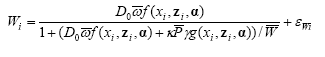
Crop yield:
2) 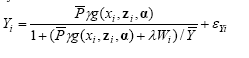
Formulas 1-2 are the primary functions, whereas formulas 3-4 are used for estimation purposes:
Weed density and biomass:
3) 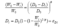
Crop density:
4) ![]()
The functions f, g, and h express the harrowing (z) and herbicides’ (x) relative effect (survival) on weed, crop yield and crop density, respectively. Theα represents local (ex post) herbicide and harrowing response parameters. Theω, μ are local (ex post) weed and crop plant weights. And the β, ρ κ λ γ andC are common (ex ante) response slopes, synergy and intra/inter-specific feedback parameters.
Herbicides relative effect (survival) on weed biomass, crop yield and crop density is calculated:
5) 
Harrowing relative effect (survival) on weed biomass, crop yield and crop density is calculated:
6) 
In the case of repeated post emergence harrowing:
7) ![]()
In case of a combination of pre- and post-emergence harrowing:
8) ![]()
In case of a combination of herbicides and post emergence harrowing:
9) ![]()
2.5.3.2 Parameter estimation and testing
Some of the model complex parameters used in formula 1-9 above have been set beforehand or estimated from findings in the literature and DJF trials included in the Crop Protection Online project (Jørgensen et al. 2007), but most of the parameters have been estimated by using the selected 32 + 9 Landsforsøg and non-linear simultaneous regression analysis using weighted least square estimation by means of the Newton-Raphton method.
The beta response parameter βx used to calculate the herbicides’ (x) effect on weed and crop in formula 5 and 9 has been set to 0.6. Experiments in the Jørgensen et al. (2007) project has shown that the beta parameter for the different herbicides varies from 0.57 to 1.33. Express (tribenuron-methyl) and Express + Oxitril (ioxynil and bromoxynil) are the most used herbicides in the 32 + 9 trials. The general beta response parameter for these herbicides has in Jørgensen et al. (2007) been estimated to 0.65 and 0.57, respectively. An additional analysis has shown, that 0.6 is a decent beta parameter for blends of herbicides including herbicides with even higher individual beta parameters.
Also the beta response parameter βz used to calculate the post emergence harrowing (z) effect on weed and crop in formula 5 and 9 has been set to 0.6. Findings from scientific articles on weed response to post emergence harrowing indicate that the harrowing beta varies from 0.53 to 0.84 with an average around 0.58 (Ørum and Rasmussen, 2007).
Modelling the weed biomass and the crop yield as a function of the weed biomass is the main task for the model complex, but unfortunately the weed biomass and the specific weed density has (as always) not been registered in the available Landsforsøg trials with mechanical weed control and barley species. To compensate for this gap, the weed biomass is estimated by using the weed density data plus knowledge and functionality established in the Jorgensen et al. (2007) project. In that project the relation between weed density and weed biomass has been analysed for more than 100 herbicide trials in spring barely, including more than 1.100 treatments and detailed registrations on crop yield and weed species density and biomass.
In the Jørgensen et al. (2007) project, the ρ parameter in formula 3, used to describe the correlation between the reductions in weed density and weed biomass from using herbicides and harrowing, has been estimated to 0.6 for herbicides (ρx). Here it is also found that the observed average untreated weed plant weight (W0/D0) is 5 g per m², and that the estimated average crop-and-weed-free weed plant weight (ω) is 10 g per m² with a 10 g per m² standard deviation.
The rest of the parameters are in principle estimated simultaneously, but in practice the parameters have been estimated in an iterative stepwise process. First the local (ex post) parameters (see table 2.7) are estimated for each location, then the common (ex ante) parameters, all the local parameters, the common parameters plus local crop and weed weights, and the common parameters and the local response parameters (see table 2.6) have been estimated. All these parameters have been estimated again and again until the weighted sum of the squared error terms (εW, εY and εD) from formula 1, 2 and 3 are minimized (stabilized).
Unfortunately none of the selected trials are dealing with sole post emergence harrowing, weed biomass has, as mentioned, not be registered and the harrowing intensities (z) have not been registered in the series 091970101 and 020280101 trials. A crop soil cover from 10 to 20% is recommended in the Landsforsøg trials, but intensity varies from trial to trial, having an average crop soil cover around 10%. If the intensity for the series 091970101 and 020280101 trials are set to high, the average effect of a 20% crop soil cover harrowing is underestimated, and if the crop soil cover is set to low, the average effect of a 20% crop soil cover harrowing is overestimated. According to Rasmussen (2004) and Odderskær et al. (2006), a 20% crop soil cover harrowing is expected to reduce the weed biomass by 70%. Due to the above mentioned shortcomings, the resulting average reduction in weed biomass from a standard harrowing can not be estimated exactly nor calculated from the selected Landsforsøg trials alone. It has been decided to estimate an average crop soil cover between 10 and 20% for the series 091970101 and 020280101 trials yielding an average 70% reduction in case of a 20% crop soil cover harrowing in all 32 trials with weed harrowing. Actually an 8% crop soil cover in the series 091970101 and 020280101 trials is needed to achieve this goal. But in order not to overestimate the weed control effect a 12.5% crop soil cover has been set for the two series, resulting in a 68% average reduction in the weed biomass. If the two missing crop soil covers were set to 5 or 20% the average effect of a 20% crop soil cover would have been 66 and 71% respectively.
Table 2.6 shows the common (ex ante) parameter estimates.
Table 2.6. Common (ex ante) parameter estimates.
| Parameter | Explanation | Weed biomass | Crop yield | Crop density |
| βx | Herbicide response (slope) | 0.6 | ||
| βZ | Harrowing response (slope) | 0.6 | ||
| ρx | How herbicides retard weed | 0.6 | ||
| ρZ | How harrowing retard weed | 0.73 | ||
| κ | Crop influence on weed biomass | 0.045 | ||
| λ | Weed biomass influence on crop | 0.6 | ||
| αYx | Crop damage from herbicides | 0.26 | ||
| C1. 2. 3… | Post x Post synergy | 0.752 | 1.09 | 0.714 |
| Pre x Post synergy | 0.05 | 0.05 | 1.25 | |
| Herbicides x Post synergy | 1.25 | 0.05 | 0.05 | |
| Aux. αp | Alpha factor Pre harrowing | 18% | ||
| Alpha factor Post harrowing | 58% | |||
| Varieties | Lux weight and yield factor | 1 | 1 | |
| Jacinta factors | 0.72 | 1.04 | ||
| Otira factors | 1.4 | 1.02 | ||
| μ | Aux. density factor | 0.973 | ||
Source: Selected Landsforsøg (Petersen, 2006).
In the Crop Protection Online (PVO) decision support system for chemical weed control (Bøjer & Rydahl 2007) used in wide range of arable crops, it is anticipated that each herbicide has only one beta parameter valid for all conditions, weed species and crops. As a parallel to this, it has been decided that also harrowing has only one, general beta response parameter valid for all conditions, weed species and crops.
The ρZ parameter used to describe the correlation between the reductions in weed density and weed biomass from using harrowing has been estimated to 0.73. This value does not differ significantly from the 0.6 found for herbicides (ρx). But, it indicates that weed treated with herbicides are more retarded than weed treated with harrowing, and that weed surviving the harrowing is more vital than weed surviving herbicides.
The synergy parameters C are used to add up the effect of more harrowing or combinations of harrowing and herbicides. According to Ørum et al. (2007), a synergy factor close to 1, like the estimated harrowing plus harrowing synergy effect on the crop yield, indicates that each harrowing is reducing the yield or weed biomass by the same factor (Minimum survival model, MSM), whereas a synergy factor close to 0.6, like the harrowing plus harrowing synergy effect on the crop density, indicates that the herbicide doses and harrowing intensity are additive (Additive dosage model, ADM). In case of a high (higher than 0.6) synergy factor, like the herbicide x post emergence harrowing effect on weed biomass (1.2), the combined effect of a low herbicide dose and a normal post emergence harrowing is supposed to be very effective. And in case of a low synergy factor (below 0.6), like the pre x post emergence harrowing effect (0.15), the weed control effect of a pre-emergence harrowing is almost lost if the pre-emergence harrowing is combined with an effective post emergence harrowing. The 0.7 harrowing x harrowing synergy factor for weed biomass indicates that the effect of splitting up the harrowing is somewhere between MSM and ADM. This could indicate, that ADM is the right model if the exact effects of the harrowings are known, and the better synergy than ADM is due to the fact that for one intensive harrowing with a good or bad timing is on average less effective than two less intensive harrowings having a good and a bad timing. In case of the harrowing x harrowing synergy factor for weed biomass right between MSM and ADM, more analyses are needed to identify the most efficient harrowing strategy.
The auxiliary alpha factors for pre- and post emergence harrowing indicate that harrowing and, especially, pre-emergence harrowing are relatively less damaging to the crop density than to the crop yield. The local pre- and post emergence harrowing alpha response parameters used to calculate the crop yield are also used to calculate the crop density, but multiplied by the auxiliary alpha.
The estimated barley varieties factors indicates, as expected, that the varietis Otira with a 1.4 weight factor is the most competitive of the three varieties, but, the varieties Jacinta and not the variety Lux is found to be the least competitive variety. The yield factors indicate that, on average, Jacinta and Otira offer a 4% and 2% higher yield potential than Lux. In this way Jacinta may still end up being more competitive or less weed depending than Lux.
Table 2.7 shows the local (ex post and stochastic) parameter estimates.
Table 2.7. Local (ex post or stochastic) parameter estimates.
| Parameter | Explanation | Unit | Average | Standard deviation | Average | Standard deviation |
| 32 herbicide and harrowing trials | 9 variety and seed density trials | |||||
| Y | Potential yield | Hkg ha-1 | 63.2 | 11.1 | 59.7 | 13.3 |
| γ | Crop plant weight | Hkg ha-1 | 12.7 | 2.3 | 9.9 | 4.9 |
| ω | Potential weed plant weight | g m-2 | 10.3 | 8.2 | 8.4 | 4.0 |
| P | Observed untreated crop density | m-2 | 242 | 54.5 | 300*) | 150 |
| D0 | Observed untreated weed density | m-2 | 103 | 92 | 241.7 | 54.5 |
| αWx | Herbicide weed response | 3.6 | 2.2 | 4.3 | 2.6 | |
| αWb | Pre-emergence harrowing weed response | 0.85 | 0.60 | |||
| αWz | Post emergence harrowing weed response | 4.8 | 1.9 | |||
| αYB | Pre-emergence harrowing yield response | 0.17 | 0.27 | |||
| αYz | Post emergence harrowing yield response | 1.1 | 0.9 | |||
*) The crop density in the variety and seed density trials are defined as150, 300 and 450 plants per m-2.
Source: Selected Landsforsøg (Petersen, 2006).
3 Results
3.1 Weeds and arthropods
3.1.1 Field experiment
3.1.1.1 Effects of harrowing on diversity of weed species
The sum of all subsample occurrences of all weed species was calculated for the reference and experimental subplots. Maximum theoretical number of occurrences per category was 135 for each species. The results are presented in Figure 3.1. After three and four times harrowing, a marked difference in weed occurrence is seen, when comparing only two harrowings with three, respectively four harrowings. Furthermore, no significant change in the weed occurrence was found, when increasing weed harrowing from three to four times harrowing (model 1).
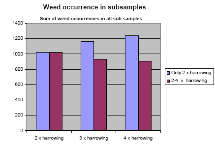
Figure 3.1. The effect of harrowing on weed occurrence. Y axis is the sum of recorded species in all subsamples.
The total number of weed species observed in all the subplots as a function of harrowing frequency is shown in Figure 3.2.
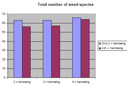
Figure 3.2. The effect of harrowing on the total number of observed weed species. Y axis: the total number of weed species observed.
There is no significant difference between two and four harrowings, but a small, not significant increase in total species number with harrowing frequency, probably reflecting the higher probability with time for new weed species to occur (see discussion). The seemingly higher difference between the columns at 2 x harrowing is only accidental.
3.1.1.2 The effect of weed harrowing on vegetation biomass
The results were analysed statistically using the model 2. The total number of samples with size 0.15 m² (mean of four - five subsamples of 0.15 m² – see Figure 2.2) was number of years ´ number of farms ´ number of plots per field ´ number of subplots per plot ´ number of samplings = 2´6´2´11´3 = 792; three of these were discarded due to anomaly.
Table 3.1. The reduction in weed and crop biomass related to number of times harrowing. The sampling in the two plots per field was carried out simultaneously ensuring that the estimated biomasses between two-harrowing plots and three-four harrowing plots are directly comparable. The % reduction in weeds is significant at the P < 0.01 level..
| Vegetation | Estimated mean dry biomass, g m-² | % reduction | ||
| Affected by 2 harrowings | Affected by 3 harrowings | Affected by 4 harrowings | Total | |
| Weeds | 3.5 | 2.0 | 43 | |
| 12.0 | 6.3 | 48 | ||
| Crop | 60.7 | 58.7 | 3 | |
| 213.0 | 200.0 | 6 | ||
It is seen from Table 3.1, that there is relatively little further weed and crop reduction by increasing the harrowing frequency from three to four times. This may infer that acceptable decrease in weed competition on the crop already was attained with only three times harrowing.
3.1.1.3 The relation between weed biomass and weed species composition
It was attempted to clarify, whether variation in weed species composition reflects differences in ecological growth conditions between the experimental plots, by Sørensen similarity and Ellenberg index calculations.
In total 81 taxons of weed plants were found in the biomass samples. In order to calculate Sørensen similarity and weighted Ellenberg indices, the biomass samples were ranked in separate weight classes. The number of intervals was 30 (Sørensen index) and 12 (Ellenberg), and the total number of biomass samples was 789. Sørensen similarity index is based on the number of species occurring in the two samples selected for comparison, and the number of common species between these samples. The index range is 0 to 1. The results are shown in the matrix (Table 3.2). One figure in the matrix is the calculated Sørensen index for the species contributing to the two compared weight classes. The bold figure 0.8 thus constitutes the Sørensen index based on the species found in weight class nr 8 (0.07-0.08 g) and 10 (0.09-0.1 g), respectively. In general terms, the index value 0.8 means that 80% of the species found in the two weight classes are the same.
Table 3.2. Sørensen similarity indices. Only indices with values equal to or higher than 0.6 are shown. Numbers 1-30 represent biomass weight intervals separated by 0.01; 0.02; 0.03; 0.04; 0.05; 0.06; 0.07; 0.08; 0.09; 0.1; 0.2; 0.3; 0.4; 0.5; 0.6; 0.7; 0.8; 0.9; 1; 2; 3; 4; 5; 6; 7 ; 8; 9; 10 and 20 g dry matter, respectively The Sørensen index is calculated as 2a/(2a+b+c) where a is the number of common species and b & c are the numbers of species only found in one of the two plots under comparison. If the value is above 0.6, more then 60% of the species are common. The matrix is filled out with few, scattered cells, where the index value was below 0.6.
Table 3.2 shows, that there is a high degree of similarity between the biomass samples with respect to weed species composition, and for most of the weight classes, there is more than 60% common species when compared in pairs. There is, based on these results, no reason to suspect any strong variation in ecological growth conditions between the experimental areas. This conclusion is corroborated by calculation of weighted Ellenberg indices, calculated for the same material. Based on the registered Ellenberg index values for the weed species contributing to the sub sample biomass values, and using the biomass of the individual species as importance value, the weighted Ellenberg indices for L, F, R and N were calculated. The results are presented in Figures. 3.3 and 3.4.
Figure 3.3. Compilation of Ellenberg indicator values (ranges1-9) of 12 biomass weight classes. L: Light, F: Humidity; R: pH (high value corresponds to high pH); N: Eutrophication with nitrogen compounds. The bars represent different weight classes between 0-1 g to >20 g biomass pr sample.
Figure 3.4. Weighted Ellenberg indices based on Ellenberg light (L; range: 1-10) and humidity (H; range: 1-10) indicator values for the weed species contributing to the biomass. Importance value: Biomass weight in g dry matter of the weed species. The x-axis is 30 weight classes from 0.01-0.02 to >20 g biomass. The F trend line slope is not significantly different form zero.
Based on the Ellenberg index results above, it may safely be concluded that no humidity gradient is present in the material. The humidity gradient was singled out, as this indicator in particular was believed to be of possible importance. A significant humidity gradient would have effect on the conclusions. In other words, high biomass values do not result from higher water availability, as the species composition of samples with high biomass does not reflect adaptation to a more humid environment.
3.1.1.4 Weed plant phenology related to harrowing frequency
Table 3.3 shows the results of the phenological studies 2004 and 2005.
Table 3.3. Statistical significant findings from the phenology analyses.
| Treatment | Number of species | Estimated relative frequencies | |
| Flowering plants/ all occurring plants |
Seedlings/ all flowering plants |
||
| 2 x harrowing | 10.0 | 0.52 | 0.11 |
| 4 x harrowing | 8.1 | 0.38 | 0.16 |
The number of species was significantly higher (25%) after only 2 x harrowing compared with 4 x harrowing. The relative frequency of flowering plants (the ratio flowering plants versus all recorded plants) was also highest (14% higher) by 2 x harrowing, while the number of seedlings was highest (5%) by 4 x harrowing. No clear conclusion with respect to harrowing frequency could be made concerning the relative frequency of seed producing plants; the results from 2004 and 2005, respectively, were contradictory.
3.1.1.5 Pin-point analyses of crops and weeds
In 2004, pin point analyses were made in all the fields after two and four harrowings. The analyses were done shortly after second harrowing and shortly after fourth harrowing, respectively. The number of times (out of the maximum 100) the pin touched either a crop or a weed shoot, respectively, was noted. One frame was analysed at all of the 11 subplots. The average values of the recorded pin-point frequencies are shown in Table 3.4. The weed data in Table 3.4 are based on hits on several species, but no distinction is made here.
Table 3.4. The average number of pin-point hits (=pin pont frequencies in %) of crops and weed plants. Frame size 1 m² with a 10 cm mesh, givng a theoretical maximum of 100 hits per stop.
| After 2 harrowings Crop |
After 4 harrowings Crop |
After 2 harrowings Weed |
After 4 harrowings Weed |
|
| Asnæs | ||||
| Four harrowing plots | 15 | 40 | 1 | 1 |
| Two harrowing plots | 14 | 47 | 0 | 2 |
| Viskingegård | ||||
| Four harrowing plots | 9 | 36 | 0 | 2 |
| Two harrowing plots | 10 | 31 | 1 | 3 |
| Vibygård SØ | ||||
| Four harrowing plots | 55 | 30 | 12 | 3 |
| Two harrowing plots | 58 | 30 | 7 | 7 |
| Vibygård NV | ||||
| Four harrowing plots | 50 | 35 | 4 | 2 |
| Two harrowing plots | 60 | 27 | 3 | 2 |
| Oremandsgård | ||||
| Four harrowing plots | 34 | 28 | 3 | 2 |
| Two harrowing plots | 36 | 30 | 3 | 3 |
| Gl. Oremandsgård | ||||
| Four harrowing plots | 60 | 43 | 18 | 10 |
| Two harrowing plots | 53 | 45 | 20 | 39 |
The plots received four or two harrowings, and all the plots were analysed when the fourth harrowing had taken place at the ‘four harrowing plots’.
The effect on the crop is marginal when inceasing the harrowing from two to four times (Table 3.4), but the effect on the weed abundance is seen in two cases: Gl. Oremandsgård (39 versus 10) and Viby SØ (7 versus 3), the former showing the strongest effect. The pattern, however, is complex, and the number of weed hits too few, so the conclusion is not statistically significant.
3.1.1.6 The effects of weed harrowing on polyphagous arthropod predators
Data from the soil flooding method were analysed using two statistical models. One model analysed if there were differences in arthropod densities between two-harrowing plots and the plots receiving three and four weed harrowings (the basic model 2). The other model included covariates (model 3). A covariate is e.g. weed biomass, which was included in the analysis in order to explain indirect (or hidden) effects behind the results obtained by the basic statistical model. Such an effect could e.g. be a higher weed occurrence in two-harrowing plots, which may influence the predator densities.
Using model 2 significant numerical responses of weed harrowing were found for Linyphiidae, Tachyporus and the sum of the four groups of polyphagous predators analysed (Table 3.5). For the carabids Agonum and Bembidion no significant effects of weed harrowing were revealed. In all significant cases higher arthropod densities were found at two weed harrowings compared to three and four harrowings (Figure 3.5). The effects of year and the interaction weed harrowing ´ year were not significant in any cases (Table 3.5), implying that the effects of weed harrowing could reliably be analysed independently of year effects.
Table 3.5. Results of the statistical tests of the density effect of three and four weed harrowings compared to simultaneous densities in two-harrowing plots of common polyphagous predators in spring wheat using the basic statistical model on soil flooding data (model 2).
| Harro- wing |
Factor | Significance (P) | ||||||||
| Agonum | Bembidion | Linyphiidae | Tachyporus | Total | ||||||
| Three | Weed harrowing | 0.4697 | 0.1127 | 0.0196* | 0.0331* | <0.0001*** | ||||
| Year | 0.2954 | 0.3884 | 0.9870 | 0.7405 | 0.9952 | |||||
| Weed harrowing´Year | 0.1348 | 0.1778 | 0.6529 | 0.2013 | 0.4133 | |||||
| Four | Weed harrowing | 0.1146 | 0.1149 | 0.0025** | 0.0320* | 0.0434* | ||||
| Year | 0.0591 | 0.1865 | 0.7346 | 0.5556 | 0.7963 | |||||
| Weed harrowing´Year | 0.7250 | 0.7042 | 0.8377 | 0.8808 | 0.6069 | |||||
*P < 0.05, **P < 0.01, ***P < 0.001
Figure 3.5. Estimated densities (Least-squares means based on the basic statistical model) of common polyphagous predators in spring wheat following three and four weed harrowings compared to simultaneous densities in two-harrowing plots. Notice the different scales on the ordinates. ns P > 0.05, *P < 0.05, **P < 0.01, ***P < 0.001.
Using model 2 the estimated densities of Linyphiidae were 51% higher at two weed harrowings compared to three harrowings. For Tachyporus this difference was 54% and for the sum of polyphagous predators a 35% higher density was found in two-harrowing plots (Figure 3.5). Following four weed harrowings the densities for Linyphiidae was 46% higher in two-harrowing plots, 32% higher for Tachyporus and 21% higher at two weed harrowings for the sum of predators (Figure 3.5).
The statistical analysis comparing the relative effects of three and four weed harrowings on arthropod abundance (model 4) revealed that there was no significant difference (P = 0.081), indicating that the relative effect on arthropod densities was the same for the third and fourth weed harrowing.
The effect of fourth weed harrowing however, may partly be explained by carry over effects from the third harrowing. Using estimates from the basic statistical model the densities of the arthropod predator complex following 3rd weed harrowing were 8.5 per m² in the two-harrowing plots and 6.3 per m² in the plots receiving three weed harrowings (Figure 3.5). Following fourth weed harrowing the predator density in two-harrowing plots was 14.4 per m² and 11.9 per m² in the plots receiving four weed harrowings. In two-harrowing plots that was a 70% increase in predator density for the time period from the third harrowings to the time period of the fourth harrowings (or 5.9 individuals per m²) and in plots receiving four harrowings that was a corresponding 90% increase (or 5.63 individuals per m²). This means, that the relative increase in arthropod densities from the time following third harrowing to the time following fourth harrowing was higher in four-harrowing plots despite the extra harrowing and the corresponding absolute increases in predator densities was approximately the same for both treatments despite the fourth harrowing. The higher relative increase in predator densities in the four-weed harrowing plots can mainly be referred to a factor four increase in Tachyporus density compared to a factor three increase in two-harrowing plots.
Model 3 included four covariates: ‘2nd weed harrowing’, ‘distance’, ‘weed’ and ‘crop’ in order to explain part of the statistical variation. ‘2nd weed harrowing’ is density of arthropod predators following 2nd harrowing. This covariate adjusts for the natural density variation within each experimental field before the third and the fourth harrowings were carried out. ‘Distance’ is the loge-transformed distance in meters to the nearest perennial vegetation from the sampling sites. This distance may affect the predator distribution within the field with fewer arthropod predators at increased distance to perennial vegetation. ‘Weed’ and ‘crop’ are the vegetation biomasses in g per sample of 0.15 m². The amount of vegetation, which in this case is measured as biomass, may affect the predator abundance.
Model 3 revealed that the third weed harrowing had a direct negative effect on densities of Linyphiidae, Tachyporus and the total number of predators (as the basic model 2) which could not be explained by the covariates because the factor ‘weed harrowing’ was still significant for these predator groups (P < 0.05) even the four covariates were included in the model (Table 3.6).
Table 3.6. Results of the statistical tests of the density effect of three and four weed harrowings compared to two weed harrowings on common polyphagous predators in spring wheat using the full statistical model including covariates on soil flooding data. Covariates with P > 0.1 were omitted from the analysis.
| Harro- wing |
Factor | Significance (P) | ||||||||
| Agonum | Bembidion | Linyphiidae | Tachyporus | Total | ||||||
| Three | Weed harrowing | 0.7356 | 0.1251 | 0.0493* | 0.0278* | 0.0003*** | ||||
| Year | 0.3094 | 0.4327 | 0.9789 | 0.8444 | 0.6810 | |||||
| Weed harrowing ´Year | 0.1712 | 0.1881 | 0.7070 | 0.0576 | 0.1732 | |||||
| 2nd weed harrowing a | 0.0140* | 0.0377* | - | 0.0027** | 0.0002*** | |||||
| 2nd weed harrowing ´Year | - | - | - | - | 0.0630 | |||||
| Distance* | - | - | - | - | - | |||||
| Distance´Year | - | - | - | - | - | |||||
| Weeda | 0.4003 | - | 0.0300* | <0.0001*** | 0.0009*** | |||||
| Weed´Year | 0.0096** | - | - | - | - | |||||
| Cropa | <0.0001*** | - | - | <0.0001*** | <0.0001*** | |||||
| Crop´Year | - | - | - | - | - | |||||
| Four | Weed harrowing | 0.6220 | 0.1042 | 0.0125* | 0.1799 | 0.3221 | ||||
| Year | 0.0565 | 0.5357 | 0.7624 | 0.0830 | 0.9725 | |||||
| Weed harrowing ´Year | 0.6880 | 0.8848 | 0.8893 | 0.7305 | 0.6815 | |||||
| 2nd weed harrowing a | - | - | - | - | - | |||||
| 2nd weed harrowing ´Year | - | - | - | - | - | |||||
| Distancea | <0.0001*** | - | - | 0.0587 | 0.0351* | |||||
| Distance´Year | 0.0008*** | - | - | 0.0502 | - | |||||
| Weeda | <0.0001*** | 0.1064 | 0.0084** | 0.0002*** | <0.0001*** | |||||
| Weed´Year | - | - | - | 0.0896 | - | |||||
| Cropa | <0.0001*** | 0.0244* | - | <0.0001*** | 0.0010** | |||||
| Crop´Year | 0.0008*** | 0.0426* | - | - | - | |||||
a Covariate
*P < 0.05, **P < 0.01, ***P < 0.001
Following three harrowings estimated Linyphiidae density based on model 3 adjusted for covariate effects were 43% higher in two-harrowing plots compared three weed harrowings. For Tachyporus this difference was 40% and for the sum of polyphagous predators the difference was 29% (Figure 3.6).
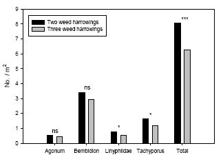
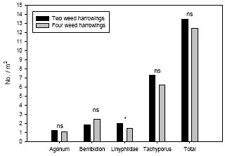
Figure 3.6. Estimated densities (Least-squares means based on the full statistical model including covariates) of common polyphagous predators in spring wheat following three and four weed harrowings compared to simultaneous densities in two-harrowing plots. Notice the different scales on the ordinates. ns P > 0.05, *P < 0.05, ***P < 0.001.
The third weed harrowing had indirectly a significant negative effect on predator densities because the covariate ‘weed’ was significantly and positively related to the densities of Agonum, Linyphiidae, Tachyporus and the sum of predators, although for Agonum there was an interaction with year (Table 3.6).
The parameter estimates revealed that when weed biomass increased with 1 g per sample (or 6.67 g per m²) the densities of Linyphiidae, Tachyporus and the sum of predators increased between 8% and 19% after the third weed harrowing (Table 3.7). For Agonum there was a positive relationship between weed biomass and carabid density in 2004 (+20% per g biomass) and a negative relationship in 2005 (- 10% per g drymass) (Table 3.7).
Table 3.7. Parameter estimates of covariates included in the full model statistical tests (see Table 3.6). Covariates with P > 0.1 were omitted from the analysis.
| Harro- wing |
Covariate | Parameter estimate ± 95% confidence limits | ||||
| Agonum | Bembidion | Linyphiidae | Tachyporus | Total | ||
| Three | 2nd weed harrowing | 0.271±0.216 | 0.174± 0.165 |
- | 0.276±0.180 | - |
| 2nd weed harrowing ´Year |
- | - | - | - | 2004: 0.105± 0.156 2005: 0.317± 0.160 |
|
| Distance | - | - | - | - | - | |
| Distance´Year | - | - | - | - | - | |
| Weed | - | - | 0.122± 0.110 |
0.192±0.066 | 0.082± 0.048 |
|
| Weed´Year | 2004: 0.200±0.126 2005: -0.102±0.192 |
- | - | - | - | |
| Crop | 0.124±0.030 | - | - | 0.101±0.022 | 0.053± 0.015 |
|
| Crop´Year | - | - | - | - | - | |
| Four | 2nd weed harrowing | - | - | - | - | - |
| 2nd weed harrowing ´Year |
- | - | - | - | - | |
| Distance | - | - | - | - | -0.173± 0.161 |
|
| Distance´Year | 2004: -1.607±0.692 2005: -0.203±0.423 |
- | - | 2004: -0.430±0.331 2005: 0.001±0.287 |
- | |
| Weed | 0.084±0.036 | 0.025±0.030a | 0.043± 0.032 |
- | 0.049± 0.016 |
|
| Weed´Year | - | - | - | 2004: 0.067±0.023 2005: 0.025±0.042 |
||
| Crop | - | - | - | 0.018±0.007 | 0.010± 0.006 |
|
| Crop´Year | 2004: 0.055±0.022 2005: 0.010±0.014 |
2004: -0.001±0.015 2005: -0.025±0.018 |
- | - | - | |
a Not significant (P = 0.1064 - Table 3.6)
The covariate ‘crop’ was positively related to densities of Agonum, Tachyporus and total number of predators after the third weed harrowing. When crop biomass increased with 1 g per sample the densities of these three predator groups increased between 5% and 12% (Table 3.7). The effect of weed on arthropod densities was in all cases higher than the effect of crop at the time following third weed harrowing except for Agonum in 2005 (Table 3.7).
Model 3 including covariates revealed that the fourth weed harrowing only had a direct negative effect on densities of Linyphiidae (Table 3.6) (or carry-over effect from third weed harrowing – see discussion). This means the significantly negative effect of weed harrowing on Tachyporus and the total predator complex found by model 2 following the fourth weeding indirectly can be explained by the covariates in model 3. The density of Linyphiidae adjusted for covariate effects was 38% higher in two-harrowing plots compared to four-harrowing plots (Figure 3.6).
After the fourth harrowing the covariate ‘weed’ was significantly and positively related to all predator groups except for Bembidion where the positive relationship was not significant (Table 3.6), revealing a significant negative effect of removing weed biomass, hence an indirect effect of harrowing on the predator groups. The parameter estimates showed that when weed biomass increased with 1 g per sample the densities of predators increased between 3% and 8% at the time when the fourth weed harrowings were carried out (Table 3.7).
The covariate ‘crop’ was positively related to densities of Agonum, Tachyporus and total number of predators after the fourth weed harrowing and negatively related to Bembidion. The crop biomass however, interacted with the factor ‘year’ for the carabids Agonum and Bembidion (Table 3.7) revealing that the effect was not uniform between years. When crop biomass increased 1 g per sample the densities of Agonum, Tachyporus and total number of predators increased between 0% and 6% (Table 3.7). When crop biomass increased 1 g per sample the density of Bembidion was unaffected in 2004 but decreased 3% in 2005.
The effect of weed was in all cases higher than the crop effect on polyphagous predators at the time following the fourth weed harrowings (Table 3.7).
Following the third weed harrowing the covariate ‘2nd weed harrowing’ (which adjusts for the natural density variation within each experimental field before the third and fourth weed harrowing was carried out) was significant for four out of five analysed arthropod groups with the exception being Linyphiidae (Table 3.6). The covariate ‘distance’ (the loge-transformed distance in meters to the nearest perennial vegetation) was not significant in any case after the third weed harrowing (Table 3.6). It is possible that an effect of distance was already explained indirectly by the covariate ‘2nd weed harrowing’. In order to test that, ‘2nd weed harrowing’ was excluded before other model reductions in supplementary analyses using model 3. This however did not result in significant effect of ‘distance’, although the estimates in most cases were negative (Table 3.8), indicating a reduced number of predators at increased distance.
Table 3.8. Test values and estimates for the effect of the covariate ‘distance’ following third weed harrowing using a reduced model were the covariate ‘2nd weed harrowing’ was excluded before other model reductions (model 3).
| Arthropods | Estimate for distance ± 95% confidence limits |
Significance (P) | |
| Agonum | -0.350±0.547 | 0.2078 | |
| Bembidion | -0.168±0.216 | 0.1260 | |
| Linyphiidae | -0.011±0.398 | 0.9569 | |
| Tachyporus | 0.036±0.305 | 0.8180 | |
| Total | -0.022±0.162 | 0.7938 | |
Following the fourth weed harrowing the covariate ‘2nd weed harrowing’ was no longer significant in any case (Table 3.6). Instead the covariate ‘distance’ was significant and negatively related to densities of Agonum and the total number of predators, although there was interaction with the factor year for Agonum, implying that the effects was not uniform both years (Tables 3.5 and 3.6). The relationship between arthropod density and distance is illustrated in Figure 3.7.
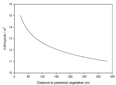
Figure 3.7. Illustration of the relationship between distance to the nearest perennial vegetation and density of the arthropod complex of polyphagous predators analysed. Only distances relevant for the described investigations are presented. Densities are not directly comparable with other arthropod densities presented due to simplicity of the illustration (back-transformed mean arthropod density vs. mean distance with the parameter estimate of distance following four weed harrowing as slope (Table 3.7).
In all cases the relative direct effect of weed harrowing was reduced in the full model (model 3) compared to the basic model (model 2) whether two weed harrowings were compared to three or four weed harrowings.
3.1.1.7 Pitfall trapping of arthropods in 2004
Pitfall trapping did generally not reveal any effect of weed harrowing, which was not found by soil flooding. Following three harrowings a significant effect of treatment was found for Tachyporus only (P = 0.002), with estimated 0.45 beetle per trapping day in two harrowing plots and 0.30 beetle in plots harrowed three times. Following four weed harrowings the factor treatment was only significant for Linyphiidae (P = 0.011), with 1.68 spiders per trapping day in two harrowing plots and 0.96 spider in plots harrowed four times.
3.1.1.8 Vegetation effect on arthropod abundance
In order to investigate the positive plant–arthropod relationships revealed in section 3.1.1.6 further, data of weeds and crop were analysed in a model excluding the direct effect of weed harrowing (models 6 and 7). The data used comprised data from two-harrowing plots only and were collected in late May and early June (the time following the 4th harrowing in the opposite field halfs) to make sure that the plots had not been weed harrowed recently thereby reducing the disturbance of weed harrowing on the analysis. Results of the statistical analyses are presented in Table 3.9.
Table 3.9. Results of the statistical tests of the relationship between vegetation biomass and densities of polyphagous predators in spring wheat using the statistical model 7.
| Factor | Significance (P) | ||||||||
| Agonum | Bembidion | Linyphiidae | Tachyporus | Total | |||||
| Year | 0.0287* | 0.5909 | 0.6657 | 0.3742 | 0.9674 | ||||
| Distancea | 0.0006*** | - | - | 0.3331 | 0.1510 | ||||
| Distance´Year | 0.0017** | - | - | 0.2733 | - | ||||
| Weeda | <0.0001*** | 0.0099** | 0.1807 | 0.0018** | 0.0008*** | ||||
| Weed´Year | - | - | - | 0.1160 | - | ||||
| Cropa | 0.0003*** | 0.3333 | - | <0.0001*** | <0.0001*** | ||||
| Crop´Year | 0.0025** | 0.0842 | - | - | - | ||||
a Covariate
*P < 0.05, **P < 0.01, ***P < 0.001
Weed and crop biomasses were also in this analysis related to predator densities because the covariates ‘weed’ and ‘crop’ (g biomass per sample of 0.15 m²) had highly significant effects on densities of Agonum, Bembidion (except ‘crop’), Tachyporus and the sum of predators (Table 3.9).
Parameter estimates of the covariates are presented in Table 3.10. For Agonum, Bembidion, Tachyporus and the predator complex there was a significantly positive relationship with weed biomass (Table 3.10). Arthropod densities increased between 2% and 8% every time weed the biomass increased 1 g per sample (or 6.67 g per m²) (Table 3.10).
Table 3.10. Parameter estimates of covariates included in the statistical model of the analysis of the relationship between vegetation biomass and densities of polyphagous predators in spring wheat (see Table 8). Covariates with P > 0.1 were omitted from the analysis.
| Covariate | Parameter estimate ± 95% confidence limits | ||||
| Agonum | Bembidion | Linyphiidae | Tachyporus | Total | |
| Distance | - | - | - | - | -0.178±0.243 |
| Distance´Year | 2004: -1.726±0.866 2005: -0.107±0.521 |
- | - | 2004: -0.292±0.416 2005: 0.001±0.388 |
- |
| Weed | 0.084±0.038 | 0.042±0.032 | 0.026±0.038 | - | 0.048±0.019 |
| Weed´Year | - | - | - | 2004: 0.067±0.025 2005: 0.023±0.050 |
- |
| Crop | - | - | - | 0.021±0.008 | 0.013±0.008 |
| Crop´Year | 2004: 0.047±0.024 2005: 0.005±0.013 |
2004: 0.005±0.019 2005: -0.020±0.024 |
- | - | - |
For Agonum, Tachyporus and the predator complex there was a significantly positive relationship with crop biomass with densities increasing between 0% and 5% at every crop biomass increase of 1 g per sample or 6.67 g per m². For the predator complex this increase was 1% (Table 3.10). The effect of weed was in all cases higher than the crop effect.
3.1.1.9 Estimating a non-linear vegetation-arthropod relationship
The data used for modelling the relationship between densities of the predator complex and vegetation biomasses excluding the influence of weed harrowing are presented in Appendix D. The result of the modelling (using model 8) is presented in Table 3.11.
Table 3.11. Estimated parameters for the model describing densities of the arthropod predator complex by vegetation biomasses and distance to perennial vegetation (model 8).
| Model Parameter |
Model | |
| Estimate | Std. | |
| α a | -7.82 | 2.49 |
| β b | 0.344 | 0.130 |
| βh c | 11.17 | 4.77 |
| γ d | 53.16 | 10.63 |
| δ e | 0.0181 | 0.0172 |
| σ2 f | 9.50 | 3.88 |
| -2 log Lg | 61.1 | |
| AIC h | 73.1 | |
| BIC i | 76.2 | |
| R j | 0.882 | |
a α = effect of distance to perennial vegetation
b β = effect of biomass
c βh = the amounth of biomass that result in an 50% effect
d γ = maximum density of arthropods
e δ = relative importance of wheat compared to weed
f σ² = residual variance
g -2 log L = - 2 log residual likelihood
h AIC = Akaike’s Information Creterion (Akaike, 1974)
i BIC = Schwarz Bayesian Information Creterion (Schwartz, 1978)
j R = Coefficient of correlation between predicted and observed values for the analyzed variable
The model can now be written as follows:
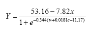
where:
Y = predicted predator density per m²
x = ln(distance in meters to perennial vegetation)
w = weeds (g biomass per m²)
c = crop (g biomass per m²)
In Figure 3.8 the observed number of arthropods is plotted against the numbers predicted by the model. In Figure 3.9 the predicted numbers of predators are shown for three combinations of the explanatory variable weed and crop biomasses and at three distances to perennial vegetation.
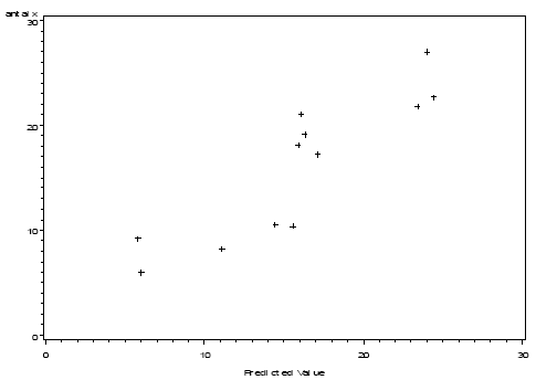
Figure 3.8. Plot of the arthropod numbers predicted by the model (X axis – no. per m²) with actual number of arthropods as response variable (Y axis - no. per m² )(r=0.88).
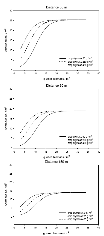
Figure 3.9. Predicted numbers of the polyphagous predator complex Agonum spp., Bembidion spp., Linyphiidae and Tachyporus spp. in spring wheat at increasing weed biomasses (dry masses) and at three distances to perennial vegetation (35, 80 and 150 m) and at three crop biomasses (50, 250 and 400 g / m²). The predictions are based on the data collected in late May and early June which are presented in Appendix D using the model presented in Table 3.11.
3.1.2 Field arena experiments
Using UV-light the positions of 80 A. dorsalis were recorded during the night observations 4 June. The results using the statistical model 9 showed an evenly distribution between the weeded and the un-weeded areas (53% vs. 47% respectively, Logit estimate = 0.1001, P = 0.6597). Only four B. lampros were seen, which was insufficient for further analysis.
On 5 June (day experiment) 273 beetles were recorded in total. Of these, 82 individuals were A. dorsalis with 68 being marked beetles. 191 were B. lampros of which 73 were marked beetles. On 11 June 191 beetles were recorded altogether with 48 being A. dorsalis and 143 being B. lampros. The results of the statistical analysis of the two day experiments are presented in Table 3.12.
Table 3.12. Summary of the statistical analysis on carabid presence on weed harrowed ground. Only the reduced models (using model 10) are presented.
| Parameter | 5 June | 11 June | ||||
| Logit estimate | Significance (P) | Logit estimate | Significance (P) | |||
| Both species (µ) | 0.0557 | 0.7374 | -1.0030 | 0.1076 | ||
| A. dorsalis (aA) | -0.2382 | 0.3340 | -1.4456 | 0.0049** | ||
| B. lampros (aB) | 0.3495 | 0.1002 | -0.6094 | 0.2154 | ||
| Species | 0.0351* | 0.0410* | ||||
| Time | -0.0836 | 0.0165* | -0.1522 | 0.1615 | ||
*P < 0.05, **P < 0.01
Table 3.12 shows that on 5 June there were no significant differences in beetle occurrence between weed harrowed and un-harrowed ground, neither for the sum of both species (µ) or for the individual species (aA and aB). However, the significant effect of difference between species indicates that there is some difference in preferences between the two species for weed harrowed and un-weeded soil. This difference is illustrated in Figure 3.10 which shows that the likelihood of finding beetles on weed harrowed ground is lower than 50% for A. dorsalis but higher for B. lampros. The significant effect of the parameter time on 5 June reveals that the percentage of recorded beetles on weed harrowed soil decreased during the day (Logit decreased by 0.0836 for every hour, Table 3.12). The vegetation biomass did not significantly influence the preferences of the beetles on 5 June in any case (P always > 0.05), and neither did any other variable analysed. If only the marked beetles recorded were analysed, the results did not differ either.
The statistical analyses of data from 11 June revealed that the probability of finding A. dorsalis on weed harrowed ground was significantly lower that 50% (Table 3.12, Figure 3.10). The probability of finding B. lampros on weeded ground was not significantly different from 50% (Table 3.12) although the estimated probability of finding the beetles was lower on weed harrowed ground (Figure 3.10). For the sum of both species there was no significant difference in preference either (Table 3.12, Figure 3.10). The significant effect of the parameter species indicates that there is some difference in preferences between species (Table 3.12), with a higher percentage of A. dorsalis preferring un-weeded ground compared to B. lampros. No of the other variables analysed were significant (P > 0.05).
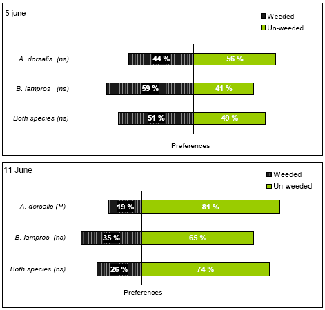
Figure 3.10. Preferences of the two common carabids A. dorsalis and B. lampros for non-weeded and newly weed harrowed spring wheat. Preference is defined as the likelihood of encountering beetles on weeded and un-weeded ground respectively. The results presented are based on two experiments carried out the 5 June and 11June. ns P > 0.05, **P < 0.01.
The results from the combined statistical analyses of the two experiments using model 11 are presented in Table 3.13. For A. dorsalis and the sum of both species there was a significantly lower preference for weed harrowed ground (Table 3.13, Figure 3.11). For B. lampros, the probability of finding the beetles on weeded ground did not differ significantly from 50% (Table 3.13), although the estimated preference for weed harrowed field was lower (Figure 3.11).
Table 3.13. Summary of the statistical analysis (model 11) of the two experiments (5 June and 11 June combined on carabid presence on harrowed ground. Only the reduced model is presented.
| Parameter | Logit estimate | Significance (P) |
| Both species (µ) | -0.4498 | 0.0136* |
| A. dorsalis (aA) | -0.7891 | 0.0135* |
| B. lampros (aB) | -0.1105 | 0.3876 |
| Both species 5 June (p5. June) | 0.0422 | 0.7740 |
| Both species 11 June (p11. June) | -0.9418 | 0.0050** |
| Date | <0.0001*** | |
| Species | 0.0377* | |
| Species ´ Date | 0.6971 | |
| Time | -0.1078 | <0.0001*** |
* P < 0.05, **P < 0.01, ***P < 0.001
The combimed analysis showed that on 11 June the sum of both species had a significant lower preference for un-weeded ground (Table 3.13, Figure 3.11), a significance which was not found when data from 11 June was tested separately (Table 3.12). Furthermore there were significant effects of the parameters date, species and time. The significant effect of species verified a difference in preference between the two species and the significant effect of time revealed that the percentage of beetles found on the weeded parts declined for every hour the sampling was carried out (Logit dropped 0.1078 for every hour – Table 3.13). No other variables analysed were significant (P > 0.05).
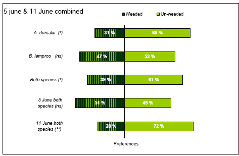
Figure 3.11. Preferences of the two common carabids A. dorsalis and B. lampros for non-weeded and newly weed harrowed spring wheat. Preference is defined as the likelihood of encountering beetles on weed harrowed and un-weeded ground respectively. The preferences presented are based on two experiments carried out the 5 June and 11 June and analysed in the same statistical model (model 11). ns P > 0.05, *P < 0.05, **P < 0.01.
3.2 Birds
3.2.1 Skylark
A total of 46 active Skylark nests were found in 2004, and 58 were found during the extended search period in 2005. The fate of the nests in each plot and year are summarized in Appendix B1. Fifty (48%) of the nests found were successful (one or more young left the nest), while 33 nests were predated, 15 were destroyed by weed harrowing and 6 failed for other reasons.
Seventeen known, active nests were exposed to weed harrowing (one of them to two harrowings). The fate of these nests is summarized in Table 3.14. In 15 cases (83%) the nest was completely lost; all eggs were removed, crushed or buried by the harrowing. Two of these nests contained 4 to 7 days old chicks, which were killed by the harrow (one of the chicks was still alive, albeit dying, two days after the event). Only in 3 cases, the nest survived, but the number of eggs/young was reduced. At the egg/young level, 55 out of 63 (87%) were destroyed while only 13% survived the harrowing.
Table 3.14. Summary of the fate of Skylark nests exposed to weed harrowing. Harrowing no. 2 was performed 11-14 May, no. 3 between 20 and 28 May and no. 4 between 30 May and 10 June.
| Weed harrowing no. | Contents at time of weed harrowing |
No. of nests exposed | Fate |
| 2 | Eggs | 3 | 3 nests destroyed |
| 3 | Eggs | 5 | 4 nests destroyed 1 nest survived: 1 egg gone, 3 intact eggs incubated |
| 4 | Eggs | 7 | 6 nests destroyed 1 nest survived: 1 egg gone, 2 intact eggs incubated |
| Eggs or newly hatched chicks | 1 | 1 nest survived: 3 chicks OK, 1 egg/chick gone | |
| Chicks | 2* | 2 nests destroyed: nestlings dead, moribund or removed |
* One of the nests had previously survived weed harrowing no. 3 (q.v.)
Weed harrowings performed = 37 days after sowing only affected known Skylark nests in two cases, whereas nests were generally exposed when harrowing was carried out = 40 days after sowing.
Rather few nests were established before mid-May, and in both study years the majority of Skylark nests were established between 15 May and 11 June (Figure 3.12). New nests were established at least until mid-July, but a clear second peak in July, corresponding to presumed second clutches, was not apparent.
Figure 3.12. Phenology of the establishing of Skylark nests on the study fields in 2004 and 2005. If a nest was found with a full clutch or with young, date of first egg was estimated from the age of the nestlings and/or the date of hatching. Notice that in 2004, nest searches stopped 3 to 4 weeks earlier than in 2005.
The density of Skylark nests and the number of eggs laid did not differ between plots that were exposed to two times weed harrowing and plots that were harrowed four times (Table 3.15). However, the number of hatchlings and the number of young leaving the nest were significantly higher in “2 harrowings” plots than in “4 harrowings” plots, indicating a higher success rate of each breeding attempt in plots that were only harrowed twice. It should be noticed that the densities in the table are minimum values (because a number of nests were certainly missed) and that first and second breeding attempts could not be distinguished with certainty and therefore were pooled.
Table 3.15. The estimated mean number of nests, eggs and chicks per ha in plots exposed to two and four times weed harrowing. Estimations and tests were based on model 13.
| No. of weed harrowings | 2 | 4 | Significance (P) |
| No. of nests per ha | 0.64 | 0.54 | 0.46 |
| No. of eggs per ha | 2.42 | 2.09 | 0.55 |
| No. of hatchlings per ha | 1.46 | 0.69 | 0.0041 |
| No. of fledglings* per ha | 1.14 | 0.40 | 0.0025 |
* Chicks leaving the nest, although still flightless at this stage
Thirty-seven out of 57 Skylark nests (65%) found in “2 harrowings” plots were successful, while this was the case in only 13 out of 47 nests (28%) found in “4 harrowings” plots. The difference in success rate is significant (P = 0.0013, model 12). By contrast, the number of fledglings per successful nest did not differ between treatments (2.89 and 2.92 in plots exposed to 2 and 4 weed harrowings, respectively).
Because the two first weed harrowings were carried out simultaneously in plots harrowed two and four times, treatment-related differences should not be manifest until after the third harrowing. To reflect this, comparisons between treatments should be restricted to nests that were active at the third harrowing or later. This constraint excluded 7 nests in “2 harrowings” plots and 2 nests in “4 harrowings” plots and increased the difference in success rate between treatments: 74% of the 50 nests in “2 harrowings” plots were successful, while only 29% of 45 nests were successful in “4 harrowings” plots (P < 0.001, model 12).
Not surprisingly, significantly more nests were destroyed by weed harrowing in “4 harrowings” plots than in “2 harrowings” plots: 26% vs. 5% (P = 0.044, model 12). However, weed harrowing mortality only accounted for part of the difference in breeding success between treatments; predation rates were also significantly higher in plots that were harrowed four times than in plots that were harrowed only twice (Table 3.16).
Table 3.16. Rate of predation on Skylark nests in plots exposed to 2 and 4 weed harrowings. Statistical significance of treatment effects on daily predation rates was tested using model 14.
| No. of weed harrowings | No. of nests | No. of nest-days | No. of nests predated | Daily predation rate | Estimated predation rate (23 days)* | Significance (P) 2 vs. 4 harrowings |
| 2 | 57 | 824 | 14 | 1.70 % | 33 % | 0.016 |
| 4 | 47 | 480 | 19 | 3.96 % | 61 % | |
| Data restricted to nests active at 3rd weed harrowing or later: | ||||||
| 2 | 50 | 802 | 10 | 1.25 % | 25 % | 0.0047 |
| 4 | 45 | 471 | 17 | 3.61 % | 57 % | |
* Calculated as 1 – (1 – daily predation rate)23
Besides the difference between plots exposed to two and four weed harrowings, it appears from Table 3.16 that predation rates were lower when only nests active at the time of the third harrowing or later were included. In fact, the daily predation rate for early nests (nests established with 1st egg no later than 20 May) was as high as 4.89% (based upon 21 nests, 184 nest-days, all plots pooled), corresponding to a total predation risk of 68% for these early nests.
It was not specifically studied which predator species were involved, but the main predator on the nests was probably Hooded Crow Corvus (corone) cornix that was frequent on most of the study fields. Predation from Crows was most important early in the breeding season when the nests were fairly easily visible. In June-July, Marsh Harrier Circus aeruginosus seemed to be an important nest predator on some of the study fields. In addition, some predation was certainly due to mustelids and other mammals.
3.2.2 Lapwing
A total of 15 and 21 Lapwing nests were found on the experimental fields in 2004 and 2005, respectively. In addition, 41 nests were found on the Vibygård study fields in 2006, and 13 Lapwing nests were found on the two Kalø fields in 2004-05. The fate of the nests on each field and treatment plot are summarized in Appendix B2. Out of the 90 nests, 47 were completely unsuccessful (all eggs lost), but in 38 nests one or more young hatched successfully and a further 5 nests were still being incubated at the end of the registration period.
By far the most frequent cause of nest failure was farming operations (27 losses, 16 because of weed harrowing, 11 because of other soil treatments). Ploughing, harrowing and rolling proved completely destructive as all nests and eggs exposed to one of these treatments were lost.
Twenty-eight active nests were exposed to one or more weed harrowings. Twelve of these nests were completely destroyed (all eggs crushed) after one harrowing. The fate of each of the other 16 nests is summarized in Table 3.17.
Table 3.17. Summary of the fate of the 16 Lapwing nests that were exposed to weed harrowing without being completely destroyed. An additional 12 nests were destroyed and abandoned after one weed harrowing.
| Year | Farm / Field | Nest ID | Contents before harrowing |
Date of harrowing1) |
Contents after harrowing |
| 2004 | Vibygård NV | B-1 | 3 eggs | 14.05 | 2 eggs gone, 1 intact egg incub. |
| B-2 | 4 eggs | 14.05 | 2 eggs gone, 2 intact eggs incub. | ||
| B-3 | 4 eggs | 14.05 | 1 egg crushed, 3 intact eggs incub. | ||
| B-4 | 4 eggs | 14.05 | 1 egg crushed, 3 intact eggs incub. | ||
| Oremandsgård | O-2 | 4 eggs | 11.05 | Nest destroyed; 1 egg gone, 1 crushed. 2 intact eggs incub. in re-established nest |
|
| 2005 | Asnæsgård | A-0 | 2 eggs | 20.04 2) | 2 intact eggs incub. |
| 2 eggs | 29.04 | Nest and eggs completely destroyed | |||
| A-1 | 4 eggs | 20.04 2) | 4 intact eggs incub. | ||
| 4 eggs | 06.05 | 2 eggs broken, 2 intact eggs incub. | |||
| Vibygård NV | B-3 | 4 eggs | 14.05 | 2 eggs gone, 2 slightly damaged eggs incub.4) | |
| B-4 | 4 eggs | 14.05 | 3 eggs gone, 1 intact egg incub. | ||
| 1 egg | 20.05 3) | Nest destroyed, abandoned. 1 egg c. 30 cm from nest, apparently intact | |||
| B-5 | 4 eggs | 14.05 | 3 eggs gone, 1 intact egg incub. | ||
| B-6 | 4 eggs | 14.05 | 1 egg gone, 2 broken, 1 slightly damaged. Incubated. | ||
| 3 eggs (2 broken) | 20.05 3) | Nest and eggs completely destroyed | |||
| B-10 | 4 eggs | 14.05 | 4 eggs more or less damaged; incub. | ||
| 4 eggs (+/– damaged) |
20.05 3) | 1 egg gone, 1 newly hatched chick, 2 partly broken eggs, incub.5) | |||
| B-11 | 4 eggs | 14.05 | Eggshell fragments – eggs crushed, predated or hatched ? | ||
| Viskingegård | V-1 | 3 eggs | 14.05 | Nest destroyed, 2 eggs intact, 1 slightly damaged. All 3 incub. in re-established nest 6) | |
| Kalø / Krovang | KR 616.33 | 3 eggs | 04.05 | 3 intact eggs incub. | |
| 3 eggs | 12.05 3) | Nest and eggs completely destroyed | |||
| 2006 | Vibygård / 5+6 | V-35 | 4 eggs | 27.05 | Nest destroyed, eggs intact but scattered. All 4 eggs later incub. in re-established nest |
1) First weed harrowing after crop emergence unless stated otherwise
2) Pre-emergence weed harrowing
3) Second weed harrowing after crop emergence
4) Both survived until time of hatching
5) One of the partly broken eggs maybe hatched
6) All 3 eggs hatched
If successive harrowings of the same nest are treated as separate events, and one nest (B-11) with unknown fate is omitted, the outcome of 33 monitored cases where a Lapwing nest was exposed to weed harrowing may be summarized as follows: 16 nests (48%) were completely destroyed (all eggs lost), 12 nests (36%) were partially destroyed (one or more viable eggs remaining, nest incubated), and 5 nests (15%) were intact (nest intact or re-established, all eggs viable, incubated). At the egg level, 116 eggs were exposed to weed harrowing; 66% of these were destroyed while 34% survived.
In several nests, more or less damaged eggs were still incubated after weed harrowing. At least in 3 cases, one or more of the foetuses were still viable:
- B-3 (2005): Incubated c. 20 days when exposed to weed harrowing. Two eggs were left in the nest after harrowing; one with just one, tiny hole, the other with 2-3 small holes. Four days later, the former was in the process of hatching and clear cheeps were heard from the egg with 2-3 holes (indicating a live young about to hatch).
- B-10 (2005): Incubated c. 18 days when exposed to weed harrowing for the first time. All 4 eggs were affected, the damage varying from tiny holes to dents c. 1 cm in diameter. The next weed harrowing was performed 6 days later, and on the following day the nest contained one newly hatched chick and two partly broken eggs. Three days later, one partly broken egg was left; the other egg possibly hatched or had been removed.
- V-1 (2005): Exposed to weed harrowing c. 3 days after the clutch was complete. All 3 eggs survived, one of them with a small crack in the shell, and the nest was re-established. On the day after harrowing, the eggs were cold when visited in late morning, but incubation was resumed one hour later. All eggs hatched successfully 24 days after weed harrowing.
The mean reproductive output per nest in relation to the number of post-emergence weed harrowings and the crop is shown in Table 3.18. Five nests (one in “1 harrowing” plots, 4 in “0 harrowings” plots) containing a total of 18 eggs were still incubated when the registrations were stopped and have been omitted from the table; these nests probably had a fair chance of being successful, thus increasing the mean reproductive output per nest.
Table 3.18. The number of Lapwing chicks (hatchlings) per nest in relation to the number of post-emergence weed harrowings and the crop. Nests abandoned with one egg and nests where the reproductive output was unknown (mainly because they were still incubated when the registrations stopped) have been omitted.
| No. of post-emergence weed harrowings | 0 | 1 | 3 | ||
| Crop | Spring-sown wheat | Spring oats with undersown grass | Perennial grass | Spring-sown wheat | Spring-sown wheat |
| No. of nests | 12 | 11 (8) 2) | 15 | 19 1) | 15 |
| No. of successful nests | 8 | 8 (8) | 12 | 4 | 5 |
| Mean no. of hatchlings per nest | 2.42 | 2.27 (3.13) 2) | 2.80 | 0.58 | 0.70 |
| Mean no. of hatchlings per successful nest | 3.63 | 3.13 | 3.50 | 2.75 | 2.10 |
1) Two nests placed in areas that were not harrowed according to schedule have been omitted.
2) 7 nests established before ploughing have been omitted. Figures in brackets also exclude nests that were established in the 5 day period between sowing and rolling.
Obviously, breeding success was greatly reduced in plots where one or more weed harrowings were performed, compared to untreated plots. The number of hatchlings per nest as well the number of hatchlings per successful nest were reduced, the latter because of partial destruction of clutches by harrowing. It appears that the success rate was higher in plots that were subject to three post-emergence harrowings than in plots that were only subject to one harrowing, but 4 of the 5 successful nests in “3 harrowings” plots were in fact only exposed to one harrowing, as the second harrowing after crop emergence on the field in question did not take place until 1 June and hatching occurred 21-29 May. Because Lapwings breed early in the season, the first weed harrowing after crop emergence is the main cause of harrowing-induced nest mortality. Out of 16 recorded nest losses due to weed harrowing, 13 were caused by the first harrowing after crop emergence and only 3 were caused by later harrowings.
In 2004 and 2005, systematic observations did not start until late April, after the emergence of the crop. This implies that nest mortalities caused by the pre-emergence weed harrowings performed between 12 and 25 April (4 to 17 days after sowing) were generally not recorded. On Asnæsgård in 2005, two Lapwing nests were found during exploratory field visits in mid-April. In these nests the first egg had been laid no later than 5 days after sowing. Both nests were exposed to a pre-emergence harrowing on 20 April and survived (cf. Table 3.17). On the other fields, no breeding Lapwings were discovered at exploratory visits around 20 April (1-2 weeks after sowing). However, on 26 April at Vibygård a nest was found with two broken and two intact eggs, probably damaged by the weed harrowing performed 8 days earlier.
On the Kalø fields, where pre-emergence harrowings were not carried out, only one or two of the 13 Lapwing nests found in 2004-05 were established before emergence of the crop (estimated from date of hatching) and would thus have been vulnerable to early weed harrowings.
In 2006, observations at Vibygård began on 7 April. The timing of the establishing of Lapwing nests varied between fields (Figure 3.13). On the two fields that were ploughed and sown in mid-April, no nests were established until early May, immediately after crop emergence (Figure 3.13 C). Thus, on these fields the nests were probably not exposed to the pre-emergence weed harrowings carried out. Contrary to this, on the large field lying as harrowed stubble until 22 April, at least 7 nests were established during the first half of April. These nests were all destroyed during soil preparation works (cf. Table 2.3). An additional 3 nests were established immediately after sowing and were destroyed by rolling 5 days after sowing. After this, 8 nests (most of them probably replacement clutches) were established within one week after rolling (12 days after sowing) and were all successful as no weed harrowings were carried out. On the perennial grassland acting as a reference area without any soil treatments, all first nesting attempts were established early, before 20 April (most of them during the first week of April), while later nests were probably replacement clutches after the first clutch had been predated or abandoned.
In at least 12 of the 90 nests found, predation was the primary cause of nest failure. Two more clutches were predated but were probably abandoned beforehand, and a further 6 clutches were partially predated as one or two eggs disappeared during incubation. In two of the 12 completely failed nests the clutch was predated over time, one or two eggs being removed between successive nest control visits until no eggs were left.
Predation rates varied greatly between fields, even on a local scale. For example, on Kalø in 2005 all Lapwing nests on the Keglehøj field were predated while all nests on the nearby Krovang field survived. However, data are too sparse to allow a detailed analysis of predation rates so only a few gross estimates can be made (Table 3.19). It appears from this table that predation rates on cereal fields and perennial grassland were rather similar and that an estimated 23% of all Lapwing nests were lost to predators while 12% of nests were partially predated.
Table 3.19. Rates of predation on Lapwing nests on the study areas. Nests abandoned early (with one egg) and nests with unknown cause of failure have been omitted from the calculations. Complete/partial predation refers to predation of whole clutch/part of the clutch, respectively.
| Crop | No. of nests / nest-days | No. of nests completely / partially predated | Daily predation rate complete / partial |
Estimated complete predation rate (30 days)* |
Estimated partial predation rate (30 days)* |
| Spring cereals | 65 / 1056 | 10 / 4 | 0.95 / 0.38 % | 25 % | 11 % |
| Perennial grass | 18 / 324 | 2 / 2 | 0.62 / 0.62 % | 17 % | 17 % |
| Total | 83 / 1380 | 12 / 6 | 0.87 / 0.43 % | 23 % | 12 % |
* Calculated as 1 – (1 – daily predation rate)30
Figure 3.13. The timing of the establishing of Lapwing nests in relation to soil treatments on the study fields at Vibygård in 2006. A: Perennial grass (no soil treatments). B: Spring-sown oats with undersown grass (1: coarse rolling, 2: ploughing followed by harrowing and sowing, 3: rolling). C: Spring-sown oats (1: ploughing, 2: sowing, 3: 1st weed harrowing, 4: 2nd weed harrowing). The oat fields were lying as harrowed stubble until ploughed. In B, one late nest (found with 4 eggs 27 May) has been omitted.
3.2.3 Oystercatcher
A total of 7 Oystercatcher nests were found (Table 3.20). Only two clutches hatched successfully while one nest was completely destroyed by weed harrowing and four were predated. Two of the predated nests had been partially destroyed by weed harrowing and were maybe abandoned before they were predated.
Table 3.20. Summary of the fate of the Oystercatcher nests found on the study fields. No nests were found in 2006.
| Year | Farm / Field | No. of eggs | Date of 1st egg (estimated) |
Date of weed harrowing | Fate |
| 2004 | Asnæsgård | = 2 | = 27.04 | 28.04 1) | = 1 egg destroyed, 1 egg intact, incub.2) Predated 7-12 days later |
| Kalø / Krovang | 2 | 02.05 | – | Hatched (2 chicks) | |
| 2005 | Asnæsgård | 3 | 29.04 - 04.05 | 05.05 1) | All eggs apparently intact, incub. Predated 19-24 days later |
| Gl. Oremandsgård | = 2 | 21-22.05 | 25.05 | = 1 egg destroyed, 1 egg apparently intact, incub.? Predated 3-9 days later, maybe abandoned beforehand | |
| Vibygård SØ | 3 | 2-3.05 | 13.05 | 1 egg gone, 2 eggs strongly damaged but incub. Predated 2-6 days later, maybe abandoned beforehand | |
| Kalø /Krovang 3) | 4 | = 25.04 | 04.05 | Completely destroyed by harrowing | |
| 3 | 12-15.05 | – | Hatched (2 chicks) |
1) Nest found on the day after harrowing
2) In re-established nest 10-15 cm from destroyed nest
3) Successive breeding attempts by the same pair
Three nests were monitored before and after weed harrowing. One of these nests was completely destroyed (all eggs lost) while the other two were partially destroyed by harrowing and may well later have been abandoned. In addition, two surviving nests were found after weed harrowing, one with 1 egg intact, the other with 3 eggs intact (Table 3.20); however, such nests should not be included in the calculation of loss and survival rates in relation to weed harrowing (cf. section 2.3.3).
The mean reproductive output was 2.0 hatchlings per nest in untreated plots and zero in plots that were subject to weed harrowing.
The daily predation rate was as high as 2.02 %, even when the two nests where predation was possibly secondary are omitted from the calculation. This is equivalent to an estimated predation rate of 46% of nests.
3.3 Weed control
3.3.1 Six field trials with repeated weed harrowings
The effect of repeated weed harrowings in spring barley has been evaluated in the selected trials described in section 2.4.1.1, and Dansk Landbrugsrådgivning concluded that an increasing number of harrowings did not increase the crop yield in spring barley (Petersen 2002).
In all eight trials, a pre-emergence weed harrowing was combined with one to four post emergence harrowings. The pre-emergence harrowing took place five days after sowing, the additional post emergence harrowings were planned to take place 7, 14, 21 and 28 days after sowing, respectively. For all eight trials the crop yield as well as the time of sowing and harrowing was reported, and for six of the eight trials the crop and weed density 14 days after the last treatment (primo/medio June) was also reported. Unfortunately the weed biomass and the intensity of harrowing were not reported.
Table 3.21 shows the effect of mechanical weeding in the selected spring barley trials.
Table 3.21. Effect of mechanical weeding in spring barley.
3.3.1.1 Yield and net yield
It is shown in Figure 3.21, that the average untreated yield is 48.4 hkg and that the highest yield, with at 0.8 hkg yield gain, is obtained by a pre-emergence harrowing plus two times post emergence harrowing. Three or more post emergence harrowings will result in a moderate 0.3-0.6 hkg yield loss. When the weeding costs are taken into account, none of the treatments are profitable. At a cost of 65 DKK per pre- and post-emergence harrowing, the increasing number of harrowings will raise the net yield loss from 1.5 to 4.6 hkg per ha. On average the mechanical weeding per se is not profitable. In this way the most efficient strategy is the one reducing the weed to a given level, involving as few harrowings as possible.
Figure 3.14 shows the net yield gain from post emergence harrowing in spring barley.
Figure 3.14. Net yield gain from post emergence harrowing in spring barley
Untreated weed density and average reduction in weed density pr. harrowing MSM is shown in parenthesis for each trial ID.
Source: Landsforsøg 2001 and 2002 (Petersen 2006, Link)
It is shown that one or two post emergence harrowings have been profitable or almost profitable for three out of six trials. For the other three trials, the net effect of mechanical weeding is negative. In these cases, the costs are increasing with the increased number of harrowings. Unfortunately there is no obvious correlation between the profitability of the treatments and weed density, and the weeding effect of the individual treatments. This indicates that in some cases, the mechanical weeding damage overrules the positive effect of reducing a high weed density, or that a high and untreated weed density not always causes a reduction in crop yield. On average a shift from a one post-emergence harrowing strategy to a three post-emergence harrowing strategy will increase the reduction in weed density from 40% to 70% and increase the weeding net cost by 1 hkg (80 DKK or 11€) per ha.
3.3.1.2 Effect on weed density
It is also shown (figure 3.14) that the first treatment reduced the crop density by 4%, the dicot weed density by 35%, and the grass weed density by 64%. In total, four post emergence harrowings have reduced the crop density by 16%, the dicot weed density by 81%, and the grass weed density by 84%.
The effect of each treatment can be calculated in many ways. A simple average effect per treatment can be calculated by dividing the total reduction by the number of treatments, and the effect can be calculated as a minimum survival effect by using the minimum survival method (MSM). According to Table 3.21 (third dicot weed column) the simple average reduction in the weed density is decreasing from 35% to 20% by increasing the number of treatments, whereas the MSM average reduction in the weed density (the fourth column) is stable and around 35%. This indicates that each post emerge harrowing reduces the remaining weed density by 35%. The average reduction per treatment calculated by using the MSM model is almost constant. This indicates that the MSM model is a god model for describing the harrowing weeding effect. It also indicates that the pre-emergence (blind) harrowing or (less likely the first post emergence harrowing) has none or little effect on the weed density. It is well known that pre-emergence weed harrowing has none or little effect on the crop, but it is also found, e.g. Rasmussen (2007), that pre-emergence harrowing in combination with post emergence harrowing has a modest and varying effect on the weed biomass. Although the pre-emergence harrowing in some cases effectively reduces the emerged weed, it also able to brings more new weed seeds to germinate.
It is found that, on average, each post-emergence harrowing reduces the weed density by 33%. In order to investigate the variation of effectiveness from trial to trial and from treatment to treatment, the total relative reduction in weed density and the logarithm to the total relative survival (100% - total relative reduction) of weed plants is shown in figure 3.15 and 3.16.
Figure 3.15. Total reduction in weed density from post emergence harrowing in spring barley. Untreated weed density and average reduction in weed density pr. harrowing (MSM) is shown in parenthesis.
Source: Landsforsøg 2001 and 2002 (Petersen 2006, Link).
It is shown (figure 3.15) that there is a huge variation in the weeding effect of post emergence harrowings. In one of the trials, a single post emergence harrowing was able to reduce the weed density by 70%, whereas in another trial four post emergence harrowings were needed to get a 60% reduction. It is also shown that high and low reductions in weed density cannot be explained alone by region (S, ØJ and VJ) or weed density (shown in parentheses).
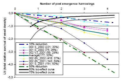
Figure 3.16. Total relative survival of weed plants for post emergence harrowings in spring barley. Untreated weed density and average reduction in weed density pr. harrowing MSM is shown in parenthesis.
Source: Landsforsøg 2001 and 2002 (Petersen 2006, Link).
It is shown (figure 3.16) that the logarithms to the total relative survival (100% - total relative reduction) of the weed density for all the trials are almost a linear function of the number of harrowings. The almost linear effect curves indicate that the MSM model is also a god model to describe the effect of repeated harrowings in individual trials. The two dashed, bold lines indicate the 66% and 16% reduction per harrowing curves. The effect of the post emergence harrowing varies from trial to trial, whereas for each trial the effect of the individual harrowings is almost constant (not varying). In other words, if the first post emergence harrowing offers a god or bad effect, the second, third, and fourth harrowing will most likely present the same god or bad effect. The bold black and gray lines indicate the 50% and 75% reduction in the weed density iso-curve. The lower the effect per harrowing, the more harrowing is needed to get a 50 or 75% reduction in the weed density. In case of the highest effect, less than one (0.8) post harrowing is needed, and in case of the lowest effect, more than two (2.2) harrowings are needed to reduce the weed density by 50%. In five of six trials, two post emergence harrowings have resulted in a 50% or higher reduction in the weed density. In all six trials three post emergence harrowings have resulted in a 75% or higher reduction in the weed density.
3.3.1.3 Effect on crop density
Also crop density is affected by mechanical weeding. Table 3.18 shows that pre-emergence harrowing plus one post emergence harrowing on average reduces the crop density by 4%, and each additional harrowing reduces the remaining crop density by 3-4%. On average, a pre-emergence harrowing plus four post emergence harrowings reduce the crop density by 16%.
Figure 3.17 shows reduction in weed and crop density in spring barley as a result of mechanical weeding.
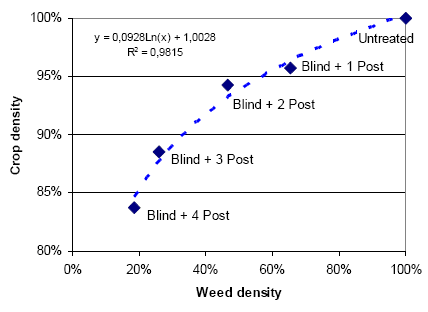
Figure 3.17. Reduction in weed and crop density in spring barley after mechanical weeding.
Source: Landsforsøg 2001 and 2002 (Petersen 2006, Link).
It is shown that weed density is much more affected by the harrowings than crop density, but it is also shown that an increased number of post emergence harrowings increases the crop damage – weed damage ratio. If it is the number of harrowings more than the intensity that causes the increased ratio, it might be an idea to perform a few but more intensive harrowings to control the weed.
3.3.1.4 Timing
It is a wide spread and often repeated assumption (e.g. Duval, 1997), that timing is alpha and omega for the weeding effect and crop damage caused by mechanical weeding. For instance, the crop is very resistant before the two-leave stage and most vulnerable in the two leave stage. Some weed spices are most resistant in the early growth stages and some are more resistant later on. The effect might also depend on the weather conditions before and after the treatment, and some treatments are able to bring more weed seeds to germinate.
Contrary to this, the above analyses (3.3.1.1 - 3.3.1.3) indicate that there is no significant timing effect. And also Rasmussen & Nørremark (2007, figure 2) found that the relative weed control (selectivity) by using post emergence harrowing in spring barley is unaffected by the crops growth stage (a two week interval from growth stage 12 to 21).
Unfortunately the selected trials do not include treatments with single pre- and post harrowings at different periods. And the first post emergence harrowings, if any, are always performed very early (7 days after sowing). By using the selected trials we can not measure the timing effect of the first post emergence harrowing. But the constant within-trial relative weed reduction (MSM)(table 3.21) and the almost straight lines in figure 3.16 indicates that timing is significantly not important for the weeding effect of at least the additional harrowings. This indicates that the post emergence harrowings, from the first to the last harrowing within each trial, independent of timing have the same relative weeding effect. In this way, the weeding effect of additional harrowings can be added up by using the MSM model, and the weeding effect of two or more post emergence harrowings can always be substituted by a single, more intensive post emergence harrowing. From a farm economic and environmental point of view, a single but intensive harrowing is optimal, and more than two harrowings, including the pre-emergence harrowing, is costly and inefficient. However, the selected data can not be used to verify whether or not timing is alpha and omega for the weeding effect of one intensive harrowing. Thus we can conclude that one intensive post emergence harrowing is optimal, and that this harrowing is expected to be an early harrowing.
Also the crop damage and crop yield may be influenced by intensity, frequency and timing of the weed harrowing. Figure 3.17 shows, that each harrowing, except for the second harrowing 14 days after sowing, reduces the spring barley plants by 5%. The harrowing 14 days after sowing seems to be less harmful than the earlier and later harrowings, and the barley is more likely to overcome the early damages by tillering etc. In that respect weed harrowings from 7 to 14 days after sowing, may be almost harmless to the crop yield. But due to shortcomings in the design of the selected field trials we can not be sure about the yield effect of intensity, timing and frequency of the weed harrowings.
As mentioned earlier, the timing of the harrowing is crucial for birds like the Lapwing and Skylarks, their nests, eggs, young and food (arthropod) for the young. Although the selected eight trials are limited to two years, no harrowings later than 28 days after sowing have been performed, these eight trials may possibly give an idea about how early the first harrowings can be carried out and how many harrowings can be performed in given periods in spring barley.
Table 3.22 sums up the timing and weeding effect of harrowing in spring barley.
Table 3.22. Timing and weeding effect of harrowing in spring barley.
| Pre emergence | 1. Post energence | 2. Post emergence | 3. Post emergence | 4. Post emergence | |||
| - Sowing - | -------------------------- Harrowing date ---------------------------- | ||||||
| 8 trials 2001-2002 | |||||||
| Day 0 | +5 days | +7day | +14days | +21days | +28days | ||
| First obs. | April 1. | April 8. | April 10. | April 20. | April 25. | May 7. | |
| Average obs. | April 13. | April 21. | April 24. | May 2. | May 12. | May 23. | |
| Last obs. | May 2. | May 7. | May 10. | May 17. | May 23. | June 14. | |
| 6 trials 2001-2002 | |||||||
| ------------- Average reduction in weed density ---------- | |||||||
| 37% | 54% | 74% | 80% | ||||
| Std.var. | (21%) | (23%) | (18%) | (15%) | |||
| ------------- Marginal reduction in weed density ---------- | |||||||
| 35% | 29% | 44% | 28% | ||||
| Std.var. | (21%) | (16%) | (17%) | (24%) | |||
Source: Landsforsøg 2001 and 2002 (Petersen 2006, Link).
It is shown that on average, the third post emergence harrowing was carried out the 12th of May, no later than the 23rd of May, and never before the 25th of April.
3.3.2 Modelling approach and more weeding trials
In this section even more but unbalanced fields trials data including chemical and mixed weeding strategies (presented in 2.4.1.2) are analysed primarily by using the complex of weed control models (presented in 2.5.1).
3.3.2.1 Weed harrowing calendar
The weed harrowing can be carried out at different periods relative to the time of sowing, the crop growth stage, the weed growth stage or the time of spraying with pesticides. Considering the Skylarks, weed harrowing should not be carried out more than 37 days after sowing and not after 20 May (see 4.2.1). The selected Landsforsøg have been used to investigate the timing of the harrowing.
Table 3.23 shows the planned and realised timing for harrowing used in the selected Landsforsøg weeding trials in spring barley.
Table 3.23. Planned and realised timing for harrowing in the selected weeding trials in spring barley 1999-2002.
| Planned treatments (timing) | Normal practice | Latest obs. |
| Barley st. 12-13 | primo-medio May | 10-May |
| Barley st. 12-14 | primo-medio May | 22-May |
| Barley st. 12-13 + 7 days | medio May | 23-May |
| Barley st. 21-25 | ultimo May | 28-May |
| Sowing + 7 days | primo May | 10-May |
| Sowing + 14 days | medio May | 17-May |
| Sowing + 21 days | ultimo May | 23-May |
| Sowing + 28 days | 1. June | 14-June |
| 5-7 days after spraying | medio May | 22-May |
| 8-10 days after spraying | medio May | 21-May |
| 16-18 days after spraying | ultimo May | 05-June |
Source: Selected Landsforsøg (Petersen 2006).
For each planned harrowing in the Landsforsøgene, the corresponding normal and latest observed timing has been deducted. The bold latest observations and treatments are those in conflict with the sky larks.
It is shown that only two types of treatments have been carried out later than the 1st of June. The treatments “Sowing + 28 days” and “16-18 days after spraying” (see also 2.4.1) are normally carried out the 1st of June and ultimo May, but in a few cases theses treatments were carried out the 14th and 5th of June, respectively. These late treatments were obtained for the fifth treatment in a five-treatment strategy, and for a combined strategy with pesticide spraying followed by a late (16-18 days) harrowing. None of the remaining mechanical strategies with less than five times harrowing (32 sites and more than 200 strategies/treatments) caused a treatment later than the 28th of May.
3.3.2.2 Standard weeding strategies
By using the above estimated model complex and the estimated local variation in crop density, yield and weeding conditions, etc., the weeding effect on weed biomass has been calculated for different herbicide and harrowing strategies. Not all of the strategies are tested in selected trials, but results are estimated by using the model complex. Table 3.24 shows the selected weeding strategies.
Table 3.24. Selected weeding strategies
| Strategy name | Short name | Pre-emergence harrowing | Herbicides | Post-emergence harrowing |
| --- No. --- | -- Treatment Freq. Index (TFI) -- | -- Crop soil cover (CSC) -- | ||
| Untreated | ||||
| Herb 0,1 TFI | Herb 0,1 | 0,1 | ||
| Herb 0,3 TFI | Herb 0,3 | 0,3 | ||
| Herb 0,5 TFI | Herb 0,5 | 0,5 | ||
| Herb 1,0 TFI | Herb 1,0 | 1,0 | ||
| Post 10% CSC | Post 10 | 10% | ||
| Post 20% CSC | Post 20 | 20% | ||
| Post 30% CSC | Post 30 | 30% | ||
| Pre | Pre | 1 | ||
| Pre + 1 x Post 10% CSC | Pre + 1 Post 10 | 1 | 10% | |
| Pre + 3 x Post 10% CSC | Pre + 3 Post 10 | 1 | 3 x 10% | |
| Pre + 1 x Post 20% CSC | Pre + 1 Post 20 | 1 | 20% | |
| Pre + 2 x Post 20% CSC | Pre + 2 Post 20 | 1 | 2 x 20% | |
| Pre + Herb 0,1 TFI | Pre + Herb 0,1 | 1 | 0,1 | |
| Herb 0,1 TFI + Post 20% CSC | Herb 0,1 + Post 20 | 0,1 | 20% | |
Figure 3.18 shows the estimated variation in weed biomass reduction for different mechanical weeding strategies in spring barley.
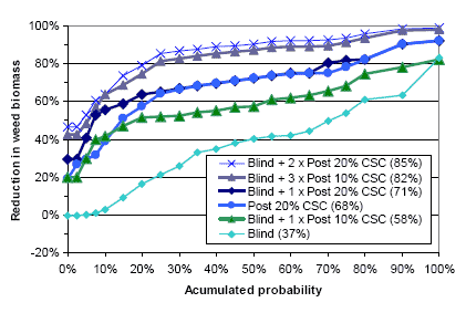
Figure 3.18. Estimated variation in weed biomass reduction for different mechanical weeding strategies in spring barley. Average reductions in weed biomass for 32 trials are shown in parentheses.
Source: Calculations on selected Landsforsøg (Petersen, 2006).
It appears that there is a great variation in the relative reduction in weed biomass for all the mechanical weeding strategies. A single pre-emergence harrowing with an average 37% reduction in weed biomass is obviously the least effective and least stable mechanical weeding strategy in spring barley. The more harrowings the higher is the relative reduction in weed biomass. A single 20% crop soil cover post emergence harrowing yields a reduction in weed biomass varying from 20 to 90%, and 68% on average. The combination of a pre-emergence harrowing and a 20% crop soil cover post emergence harrowing is, in most cases, as effective as the sole 20% crop soil cover harrowing. In some cases (less than 20% of the cases) the combination yields a 20% higher (50% instead of 30%) reduction in weed biomass, whereas, on average, the combination just yields a 3% higher reduction (71% instead of 68%). The combination of pre-emergence harrowing and one 10%, three 10% or two 20% crop cover post emergence harrowings on average yields a 58%, 82% and 85% reduction in the weed biomass, respectively. This indicates that one or two highly intensive (a high crop soil cover) harrowings are probably more (economically) efficient than three or more less intensive harrowings.
Figure 3.19 shows estimated variations in weed biomass reduction for different weeding strategies, including herbicides in spring barley.
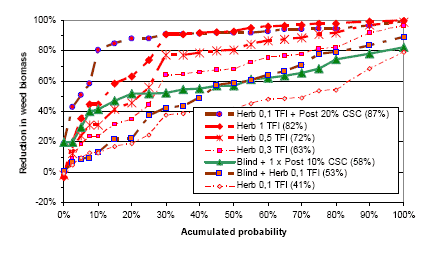
Figure 3.19. Estimated variation in weed biomass reduction for different weeding strategies, including herbicides in spring barley.
Average reductions in weed biomass for 32 trials are shown in parentheses.
Source: Calculations on selected Landsforsøg (Petersen, 2006).
It is shown that there is also a huge variation in the weeding effect of weeding strategies, including herbicides. The most effective strategies are the full dose herbicide strategy and the strategy combining a low herbicide dose and a 20% post emergence harrowing yielding an 87 and 82% reduction in the weed biomass. The least effective strategies are the 0,1 TFI low dose herbicide strategy and the strategy combining a pre-emergence harrowing and a low dose of herbicides, yielding a 41 and 53% reduction. Obviously, the weeding effect of the combination of herbicides and harrowing very much depends on the timing of the harrowing. On average they are as effective as the 0,3 TFI herbicide strategy, but used the right way, a low dose herbicides followed up by a harrowing at least a week or two after the spraying, the combination is more effective than a full dose of herbicides, or four to five intensive harrowings. The poor weeding effect of the pre-emergence harrowing followed by a low herbicide dose could, as also suggested by Petersen (2002), be caused by the pre-emergence harrowing causing new weed seed to germinate, and that the resulting new weed plants are not in the vulnerable two- leave state when herbicides are applied. The success of the low dose of herbicides followed by a post emergence harrowing could be that the weed plants surviving the herbicide treatment are retarded and weakened and thus more sensitive to the physical damage caused by the harrowing and easier to cover with soil when harrowing.
In order to pinpoint the most efficient strategy, one has to consider the costs of herbicides, spraying, and harrowing as well as yield reduction from harrowing, herbicides or weed. If there were no weed, the farmer could avoid weeding costs and yield losses from weeding. If there is a lot of weed, there will be a significant yield loss, or need for costly chemical and mechanical weeding, also damaging the crop. In the following economic analysis of the weeding strategies, the strategies are evaluated on their net cost for weed and weeding and their effect on the weed biomass. The price for a full herbicide dose (1 TFI) is set to 200 DKK per TFI. The price for spraying and harrowing is 65 DKK per ha, and the barley price is 80 DKK per hkg.
Figure 3.20 shows estimated net weed and weeding costs for a few effective weeding strategies in spring barley.
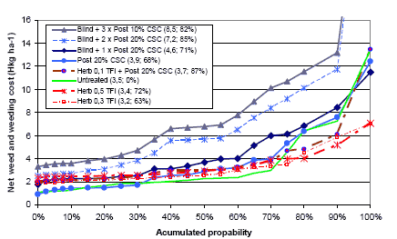
Figure 3.20. Estimated variation in net weed and weeding costs for a few effective weeding strategies in spring barley.
Average net cost and reductions in weed biomass for 32 trials are shown in parentheses.
Source: Calculations on selected Landsforsøg (Petersen, 2006).
It is shown, that there is a huge variation in the net weed and weeding cost for all the weeding strategies, however the 0.3 and 0.5 TFI herbicide strategies are significantly more stable than the strategies involving harrowing. The 0.3 and 0.5 TFI herbicide strategies and the untreated strategy are the cheapest strategies yielding a 3.2, 3.4 and 3.5 hkg per ha net cost. More harrowings results in significantly higher net weed and weeding cost. There is no correlation between net expences and the weeding effects. Some of the cheapest strategies, like the 0.5 TFI strategy, are very effective, whereas others, like the untreated strategy, have no effect at all. To pinpoint the most effective strategies both cost and effect has to be taken into account.
Figure 3.21 shows estimated net weed and weeding cost, and weeding effect for different weeding strategies in spring barley.
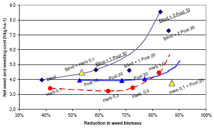
Figure 3.21. Estimated net weed and weeding cost, and weeding effect for different weeding strategies in spring barley.
Average net cost and reductions in weed biomass for 32 trials are shown in parentheses.
Source: Calculations on selected Landsforsøg (Petersen, 2006).
It is shown, that the net weed and weeding cost in most cases, except for herbicides, increase with increasing reduction in weed biomass. For the herbicide strategies, the total net cost has a minimum around the 0.3 TFI dose. In case of a required reduction in the weed biomass below 80%, the herbicide strategies are in general the most efficient strategies. If a higher reduction in the weed biomass is needed, the strategies involving post emergence harrowing, perhaps combined with low doses of herbicides, are more efficient. The 0.1 herbicide plus a 20% crop soil cover post emergence harrowing combination offer an extremely high reduction in the weed biomass, but it is a little more expensive (0.5 hkg or 40 DKK per ha) than the sole 0.3 or 0.5 TFI herbicide strategies. For farmers not using herbicides, a single intensive post emergence harrowing seems to be the most efficient strategy. A single 20-30% post emergence harrowing is more effective than the often recommended 0.3 TFI herbicide solution, indicating that such a strategy will yield the required weeding effect (70% is often supposed to be the required reduction in weed biomass).
3.3.3 Weed cost and yield loss
Yield loss is caused by weed and weeding. The yield loss from weed is often calculated as a simple difference between the full (or highest) herbicide dose yield and the less weed-controlled yield (e.g. Milberg & Hallgren 2004). In that case the controlled-weed yield and not the weed-free yield potential is the yield-loss reference. The yield loss from the surviving 20-25% weed biomass in the full dose reference is in this way “free” and not accounted for.
A new decision support system prototype for herbicides in spring barley taking care of the “free weed” problem has been tested in the Crop Protection Online (PVO) project (Jørgensen et al. 2007). In that prototype the short run economic objective is not just to maximize the net yield gain by controlling the weed, but to minimize the total weeding and weed costs. The optimal herbicide dose is unaffected, but the true cost of controlled as well as uncontrolled weed is exposed.
In Milberg & Hallgren (2004) and the Crop Protection Online (PVO) prototype the general weed yield-loss relations are set up regardless of crop density and varieties, soil type, and weed-free yield-potential etc. In Milberg & Hallgren each type of cereals has an individual (predictable) yield-loss relation, and in the Crop Protection Online (PVO) prototype each year and location has an individual (stochastic, not explained) yield-loss relation.
In the prototype the resulting fresh weed biomass (g ha-1) is a function of weed density (d), fresh weight (g) (g m-2) per weed plant, and the local (stochastic) weed conditions (T):
3.1) 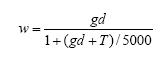
In spring barley the T-value is around 1.050 in the 15% fractal, 3.600 on average, and 12.600 in the 85% fractal. And the offset fresh weight per weed plant (g) is 10 g per weed plant per m² for an average mix of weed species. In the same prototype the yield loss (YL) (hkg ha-1) is a function of fresh weed biomass (w) (g m-2):
3.2) ![]()
By using the model complex, the yield loss depends on more than just the weed biomass, and the weed biomass itself also depends on a number of parameters. By using the model complex, the variety, seed density, weeding intensity etc has to taken into account. By using standard doses or economic optimal doses (Crop Protection Online) a 70-90% reduction in biomass is expected. Figure 3.22 shows estimated yield loss as a function of not controlled (untreated) weed biomass.
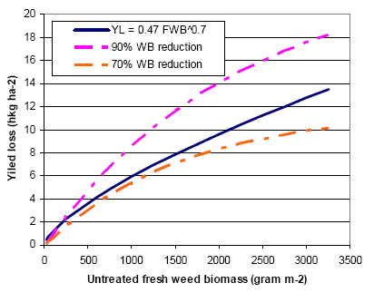
Figure. 3.22. Estimated yield loss in a 60 hkg yield potential, 250 crop plants per m-2 standard spring barley variety.
The figure shows, that an untreated 1.500 g fresh weed biomass will cause a 7, 8, or 11 hkg yield loss in case the losses are calculated by using the model complex at a low weeding intensity (70% effect, Yellow), the average Jørgensen et al. (2007) model (Blue, formula 3.1 and 3.2), or the model complex at a high weeding intensity (90% effect, Red) respectively. At a high weeding intensity, the controlled, but not weed free reference yield is higher, and thus the yield loss from not controlling the weed becomes higher. Apparently the simple yield loss (Blue) is very similar to the yield loss calculated by using the complex model on a standard barley variety with a normal yield potential (60 hkg) and seed rate (250 m-2) in case of no control and a (normally considered economically optimal) 70% reduction in the weed biomass. In scenarios where variety, seed rate, yield potential, and control measures (70% reduction) is not to be changed or discussed, the simple model (Blue line) might be as good as, and more handy, than the complex model. But we always have to remember, that the simple yield loss is not the loss compared to a weed free situation, but a situation where the weed biomass is reduced 70-80% by means of herbicides or mechanical weeding. The above figures show the yield effect caused by the barley-weed competition. The potential yield loss from using herbicides or mechanical weeding is not included in this figure and calculations.
3.3.4 Arthropods and weed costs
It is found that the number of arthropod predators (insects etc.) per m² is a function of the fields’ average weed biomass and the average distance to perennial vegetation (see 3.1.1.9). And the maximum number of arthropod is produced for a weed biomass around 15-20 g per m².
Figure 3.23 shows the estimated weed biomass as a function of weed density for a normal mix of weed species and normal (p=50%) as well as extreme weed conditions (p=15% and 85). The weed biomass is estimated by using functionality and findings from the Crop Protection Online (PVO) herbicide prototype (Jørgensen et al. 2007).
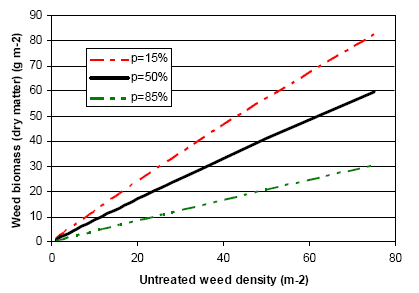
Figure 3.23. Weed biomass as a function of untreated weed density and varying weed conditions.
It is shown that in order to produce 15 g weed dry matter a weed density between 15 and 45 plants per m² is needed, depending on the weed species and the general growth conditions. A weed density around 10 to 35 plants per m² is needed to produce the maximum number arthropods, but a much higher initial weed density is of course required if the weed is controlled by herbicides or harrowing.
In order to assess the actual level of weed density and biomass in Danish fields, data from 128 field trials in spring cereals (Jørgensen et al. 2007) has been analysed (Figure 3.24). These trials are typically placed on well managed conventional arable clay soil farms on Zealand. These particular farms are considered to have low or moderate weed populations.
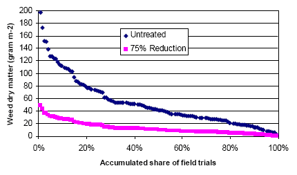
Figure 3.24. Distribution of untreated and treated (75% reduction) weed biomass (15% dry matter) for 128 spring cereal field trials.
The figure shows that almost 80% of the spring cereal fields have a sufficient untreated weed dry matter (>20 g) to insure a high density of arthropods. It is also shown, that in case of a 75% reduction in the weed biomass, less than 30% of the spring cereals fields can insure the highest density of arthropods.
Additional analysis (Figure 3.25) have shown, that 90% of these fields have an untreated weed density above 15, and 60% have a weed density above 50 plants per m².
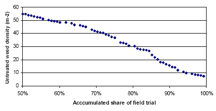
Figure 3.25. Distribution of untreated weed density for 128 spring cereal field trials.
All in all it can be concluded that even well managed conventional spring cereal fields on clay soil, in case of a reduced weed control, have a high potential for producing sufficient weed for a high arthropod predator density.
Figures 3.26 and 3.27 show weed and weeding costs (yield equivalent) estimated by using the complex of weeding models (2.5.1), and the Protection Online (PVO) prototype method (formula 3.1 and 3.2) with an average setting for weed species mix and weed growth.
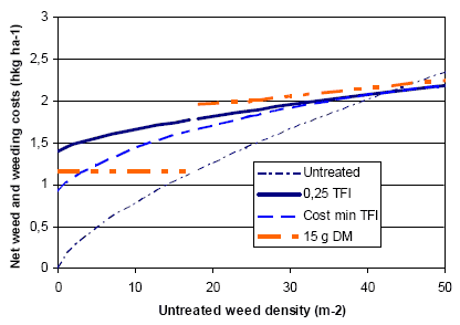
Figure 3.26. Weed biomass as function of initial untreated weed density.
Figure 3.26 shows the net weed and weeding costs in case of no weed control (Untreated), a cost minimizing herbicide strategy (Cost min TFI), a 0,25 TFI herbicide strategy, and a “15 g weed dry matter” strategy (15 g DM). Just in case of no weed and no weeding (Untreated) the net weed and weeding cost are zero. In most cases the net costs increases by increasing initial weed density. For weed deities below 40 plants per m² the no weeding strategy generates the lows net costs. On average a 17 plants per m2 weed density is required to produce 15 g weed dry matter and a high number of arthropods. At a density below 17 the “15 g dry matter” strategy requires that extra weed is “planted”. The extra plants results in more weed biomass and an extra yield loss, but weeding is not necessary. At a density above 17 the desired 15 g dry matter is produced by using reduced herbicides doses. The use of herbicides affords a spraying (result in a discontinuous curve) and the reduced (not optimal) dose and more surviving weed biomass, as in the case of the 0,25 TFI strategy, result in higher net costs.
Figure 3.27 shows the additional costs of producing the desired 15 g weed dry matter.
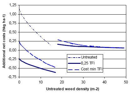
Figure 3.27. Additional net cost of producing 15 g weed dry matter relative to three different weeding alternatives.
It is shown that the additional cost of producing an average of 15 g weed dry matter depends on the initial weed density and the strategy used to produce the biomass. The additional cost (yield equivalent) of producing the desired 15 g weed dry matter at a weed density of 20 plants per m² is around 0.2-0.25 hkg (~ 2,3 € per ha) and the cost decreases to (and below zero) for an increasing weed density. In case of a very low weed density, the net costs of implantation the weed needed depends on the alternative strategy. If no weeding is the alternative the desired 15 g dry matter costs 1.25 hkg per ha (~12 € per ha), and if a 0.25 TFI herbicide strategy is the alternative, the net costs are negative.
In case of a low initial weed density, the weed biomass desired by the arthropods and sky larks can not be produced. But the above analysis have shown, that in case of a sufficient initial weed density the cost of producing more weed and to assure a high production of arthropods is very small (free or max 2,3 € per ha at the highest) and in practice insignificant for the farmer.
Additional analysis have shown that 20 and 25 g of weed dry matter also can be produced for free or at the highest for an extra cost of 0.33 and 0.5 hkg per ha (3.1 and 4.6 € per ha). Although it seems to be all most costless to produce more weed and arthropods, the farmer might still be worried about the long-run dynamic effect of producing more weed. Figure 3.28 shows the relative weed biomass reduction for different herbicide strategies.
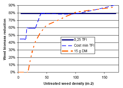
Figure 3.28. Weed biomass reduction for different herbicide weeding strategies.
It is shown, that the 0.25 TFI herbicide strategies secures a high 80 % reduction of the estimated weed biomass for all densities. Contrary to this, the “15 g weed dry matter” strategy results (not surprisingly) in a very low reduction in case of a moderate weed density. At a higher weed density the difference in weed reduction is however levelled-out.
The long run effect of a “15 g weed dry matter” strategy has not been analysed in details. But the long-run economic and dynamic effect of such a strategy will, as mentioned before, depend on the crop rotation and the weeding strategies used in the subsequent crops.
4 Discussion
The present project has focused on two major questions that have often led to discussions when chemical and mechanical weed control have been compared. One of these was an indication from a preceding project which shed light on the phase of conversion from conventional farming to organic farming, one of the changes being replacing chemical weed control with mechanical weed control (Navntoft et al. 2003). The indication of interest was that mechanical weed control might have adverse effects on beneficial soil-dwelling arthropods. These beneficials prey upon pest species providing ecosystem services of economic importance for the farmers (Östman 2003) and are also serving as prey for birds. The other debate area was the fate of bird nests during the operations of mechanical weed control. Both for the direct effects on invertebrate fauna and on bird nests as well as for the indirect effects (like, e.g., loss of bird food) more damage was anticipated after several than after few harrowings. By comparing two, three and four weed harrowings, and in addition including other weed control results in the modelling, the project results show effects on wild plants, the crop, the yield, arthropods and ground-nesting birds.
4.1 Weeds and arthropods
More than two weed harrowings had significant effects on flora and arthropod fauna in the experimental fields. The weed biomass decreased 43% after three weed harrowings when compared to two harrowings and as much as 48% after four harrowings compared to two. Along with the change in biomass, also a marked difference in weed species occurrence was seen at the high treatment level compared to only two harrowings.
The findings from the phenological studies with respect to the impact on flowering frequency and seedling frequency, respectively, may be explained in two ways. Firstly, there might be a sublethal effct on the plants due to harrowing (much like the effects of low dosages of herbicides); when the weed plant once has been covered by soil, the chance diminishes for this plant to reach maturity, make flowers and set seeds. Secondly, more seedlings may be provoked to germinate by the harrowing, but they fail to reach maturity due the late time for germination. Only the latter explanation is substantiated by the analysis of the field data obtained in this project.
The observations seem to indicate, that higher harrowing frequency reduces the number of weed plants by delaying the development of surviving plants, thus reducing flower and seed production. High weeding frequency thereby results in lower above ground weed biomass as well.
Weed harrowing had a significant negative effect on numbers of the arthropod predator complex Agonum spp., Bembidion spp., Tachyporus spp. and Linyphiidae. Shortly after the third harrowing the total density of these predators was 35% higher in plots where only two harrowings had been carried out, and shortly after the fourth harrowing this difference was 21%. The spiders Linyphiidae were the most vulnerable to weed harrowing showing a direct negative response to treatment after both third and fourth harrowing, probably as the result of a lethal effect on the mechanical operation as supported by findings of Thorbek and Bilde (2004). The rove beetles Tachyporus spp. were also vulnerable to weed harrowing, responding significantly and directly following the third harrowing. The ground beetles Agonum spp. and Bembidion spp. were the least sensitive to weed harrowing since they did not respond significantly directly to weed harrowing.
The third weed harrowing was more detrimental to the polyphagous predators than the fourth harrowing. Non-crop vegetation cover may provide an attractive foraging and resting site, which is particularly valuable prior to canopy closure (Lee & Landis 2002). This means that the arthropods may be more vulnerable to early weed harrowings carried out when the canopy is relatively open, which might explain the stronger effect of the third weed harrowing. We do not know, however, how much of the negative effect of weed harrowing after the fourth harrowing that can actually be explained by carry-over effects of the third harrowing. The findings of Thorbek & Bilde (2004) indicated that recolonization of spiders following weed harrowing eliminated the direct negative effects of the treatment within seven days. Also for carabids and staphylinids there were indications that immigration following weed harrowing compensated for direct negative effects of harrowing within a week (Thorbek & Bilde 2004).
Weeds were very important for the presence of beneficial arthropods, and weed harrowing was therefore also indirectly harmful to the beneficials. The negative effects of weed harrowing could be explained by the change in plant biomass since there was a highly significant, positive relationship between vegetation biomass (weeds and crop) and arthropod densities, with weeds having the highest positive effect on arthropod densities. An extra 1 g biomass of weed per sample could increase the density of the predator complex with up to 8 %. The importance of the vegetation was further emphasised by the statistical analysis of the effect of four harrowings because inclusion of the covariates ‘weed’ and ‘crop’ biomasses replaced the treatment effect of weed harrowing. The three predator taxa Agonum spp., Linyphiidae and Tachyporus spp. all responded positively to a higher vegetation biomass. For Bembidion spp. a significantly increase as a result of higher weed biomass was only found when data from two harrowing plots was analysed separately; in fact, a significant negative relationship between Bembidion densities and crop biomass was revealed. The contrary response of Bembidion spp. is in line with the findings of Mitchell (1963), who found that the common B. lampros had a preference for sparse vegetation (maybe because of a need for warmer soil). However, this response of B. lampros is not typical of the predatory ground beetle complex of the field taken as a whole (Speight & Lawton 1976).
Experiments with A. dorsalis and B. lampros (field arena experiments) gave further evidence that indirect effects of weed harrowing on ground beetles is species dependant. A. dorsalis had a preference for un-harrowed ground, which is in line with its positive relationship with weed biomass, whereas B. lampros had no preference for harrowed or un-harrowed ground, a result that is also in line with the observations from the larger field experiment. The probability of finding the ground beetles on the weed harrowed halves decreased during the day (as shown by the significant, negative parameter ‘time’ in Table 3.13). We do not have a bulletproof explanation, but it may be taken as an indication that the beetles had an increasing preference for undisturbed microhabitats during the day, maybe because of increasing temperatures. Honek (1997) revealed that epigaeic predators preferred shaded control stands at air temperatures of 18-25°C, while at temperatures below 16°C the catches on shaded and bare ground surface were similar. This may explain the relatively evenly distribution between weed harrowed and undisturbed soil found in the field-frame experiment on 5 June, which was a rather cool day with showers, and the strong preference for un-harrowed soil revealed for A. dorsalis on 11 June, which was warm and sunny.
The significant, positive relationship between beneficial arthropods and weed biomass made it possible to draw up a non-linear model which may be useful in the implementation of farming strategies that favour enhanced predation in spring cereal fields.
Other investigations have also revealed a positive effect of weeds on beneficial arthropods. Speight & Lawton (1976) demonstrated that beetles exerted a higher predation pressure on artificially placed fruit fly pupae (Drosophila) in weedy and presumably more humid fields. They observed a positive correlation between ground beetles and Poa annua L. and found that the underlying mechanisms were probably complex, but that is was likely that the weeds protect the predators from extremes of climate, i.e. insolation during the day and desiccation both during the day and at night. Rivard (1966) found higher catches of carabids in area of higher humidity and Powell et al. 2004 found further indications that there is a negative relationship between the majority of the epigael invertebrates and soil moisture in the summer. These findings might suggest that our results were mainly due to an arthropod – humidity relationship rather than an arthropod – weed relationship. We carried out analyses (Sørensen similarity and weighted Ellenberg indices, section 3.1.1.3) in order to test this possibility. Weed species composition reflects differences in ecological growth conditions e.g. differences in soil humidity. Differences in weed species composition should therefore unveil underlying growth conditions. There was however no indications of a different weed species composition as a result of more humid soil (e.g. in lower parts of the fields) as tested by weed species index calculations, and the positive relationship between weed biomass and important arthropods can be regarded as undisturbed this factor. This means that positive effects of the weed itself (e.g. an improved microclima) most likely is an important variable for the occurrence of generalist arthropod predators.
In addition to microclimatic considerations, it is also possible that there is an indirect effect operating via the abundance of natural prey, which may be more common in the denser patches of weed (Speight & Lawton 1976). Potts & Vickerman (1974) found a positive relationship between the numbers of predatory Coleoptera in cereal fields and the abundance of macroscopical Isotomidae (Collembola). Also Hawthorne & Hassall (1995) demonstrated that carabid density was positively correlated with the density of the prey items Collembola and aphids, besides being positively correlated with the vegetation cover. Pearce & Zalucki (2006) however, found that predator aggregation did not correlate consistently with pest aggregation, plant damage or predation rate. Collembola can be inhibited by dry microclimates (Basedow 1994). Mechanical weed control may therefore indirectly have a negative impact on the complex of polyphagous predators through a negative effect on alternative prey. However, Odderskær et al. (2006) found no negative effects of weed harrowing on densities of Collembola in organic spring wheat. This may be taken as an indication that effects of weed harrowing on alternative prey may not have influenced the distribution of the polyphagous predators in the present experiment.
The distance to perennial vegetation e.g. field margings is important for the dispersal and distribution of generalist arthropod predators in arable fields (Coombes & Sotherton 1986), a result that was also found in this experiment, based on data following the fourth harrowing. However, following the third harrowing the effect of distance to perennial vegetation was insignificant, even the estimates of the effects of distance were in most cases negative indicating that predator densities also in this case decreased at increased distance to field margins.
Generalist arthropod predators are especially important early in the growth season when specialist enemies are not yet present (Ekbom et al. 1992) These predators act as natural enemies of crop pests (Sunderland 1975), and their presence in the field early in the season can reduce the build up of pests such as the bird cherry-oat aphid (Rhopalosipum padi L.) in spring cereals (Ekbom et al. 1992). The population build up of R. padi in spring cereals usually starts late May and early June (L.M. Hansen pers. comm.). It is therefore important that the number of arthropod predators is as high as possible at that time for high natural control of aphids. To ensure a time period of one week for recolonization of predators (Thorbek & Bilde 2004), harrowing should not take place later than mid May. This should allow the population of predators to recover before aphid build up. In all cases the 2nd weed harrowing was carried out by mid May in this experiment (Table 2.1).
The present experiments only concern effects on adult individuals of polyphagous predators. Soil tilling may also affect juvenile stages (larvae and pupae) negatively. Juveniles occurring in the soil during the time of weed harrowing are often offspring of “autumn-breeders” that will emerge as adult beneficials in the field later in the season. It is also important that densities of these predators remain high later in the growth season, when they may impact pests such as Grain Aphids (Sitobion avenae (F.)) (Holland & Thomas 1997). The effect, if any, of weed harrowing on the juvenile beneficials is unknown.
For the promotion of early-occurring beneficial arthropods, and based upon the results of the present experiment, we suggest that weed harrowing is carried out early and limited to an absolute minimum and that more weed should be tolerated in the fields; the modelling indicates up to approximately 15 - 20 g weed biomass per m² in spring wheat should be allowed based on data collected in late May and early June (Figure 3.9).
4.2 Birds
4.2.1 Skylark
The number of hatchlings and the number of chicks leaving the nest were two to three times higher in plots exposed to two weed harrowings than in plots exposed to four harrowings. The significant difference in Skylark productivity between treatments was due to a higher percentage of nests being successful in “2 harrowings” plots than in “4 harrowings” plots (65% vs. 28%), whereas neither the number of nests per ha nor the number of chicks per successful nest differed between treatments.
Only 5% of the Skylark nests found in “2 harrowings” plots were destroyed by weed harrowing whereas this was the case in 26% of the nests in “4 harrowings” plots. In the latter plots, an additional 4% of the nests were exposed to harrowing but survived with a reduced number of eggs/young. Weed harrowing was generally destructive to the nests affected: 83% of the nests and 87% of the eggs or nestlings that were subject to harrowing were lost. In a study where artificial Skylark nests with eggs of Coturnix chinensis were exposed to weed harrowing, Odderskær et al. (2006) found that 72% of the nests were destroyed by a single harrowing.
In total, only 16% of the monitored Skylark nests were exposed to weed harrowing because most harrowings were performed before the number of Skylark nests peaked. The first post-emergence harrowing (weed harrowing no. 2) affected only 3 nests, whereas no. 3 and 4 affected 5 and 10 nests, respectively, although they were performed on just half of the area. Generally speaking, harrowings performed 37 days or less after sowing affected very few Skylark nests while the harrowings performed 40 days or more after sowing clearly put Skylark nests at risk. In the study of Odderskær et al. (2006), where the last harrowings were carried out 33-38 days after sowing, only two natural Skylark nests with eggs (and 3 without eggs) out of 92 nesting attempts were affected by weed harrowing. Odderskær et al. concluded that the direct, negative effect of weed harrowing on the reproductive output was insignificant, which is generally in accordance with the results from the “2 harrowings” plots in the present study.
In “2 harrowings” as well as in “4 harrowings” plots, predation was the most important cause of nest losses. Contrary to Lapwings and Oystercatchers, Skylarks have no active defence against predators and rely solely on their camouflage. Predation rates were particularly high early in the season with an estimated 68% of nests established before 21 May being predated. Later in the season, the frequency of predation was significantly higher in plots that were subject to four times weed harrowing than in plots that were harrowed only twice; the estimated predation rates were 57% and 25%, respectively. The risk of predation seems to be highly dependent on the vegetation cover. Early in the season, ground cover is sparse and the nests are fairly easily visible. Later, the higher risk of predation in “4 harrowings” plots suggests that the less developed weed cover caused by the extra harrowings makes the nests more visible to predators, probably aided by changes to the crop structure for a few days after harrowing.
The main predators were surely Crows, especially early in the season, but, interestingly, Marsh Harrier turned out to be an important nest predator in late season in some fields. Being adapted to foraging in reedbeds, Marsh Harriers seem able to localize the Skylark nests even in high vegetation, provided the ground cover is not too dense.
Overall, the difference in nest success rate (and thus in productivity) between treatments was due to the combined effects of a higher direct nest mortality caused by weed harrowings and a higher frequency of nest predation, probably due to the less developed vegetation cover, in “4 harrowings” plots.
The impact of weed harrowing on Skylark breeding success in spring-sown wheat thus depends strongly on the timing of the harrowing and the number of harrowings performed:
- Pre-emergence harrowings do not affect breeding Skylarks; the earliest known nests were established with 1st egg 18 days after sowing and never before 30 April.
- Weed harrowing performed during the first 3 weeks after crop emergence, or until 35-40 days after sowing, destroy a few Skylark nests, but the biological significance of these losses is most probably low because a high proportion of such early nests are anyway predated. Also, the height and density of the crop are still optimal for Skylark breeding so that replacement clutches have a good chance of being successful.
- Weed harrowing should not be carried out more than 37 days after sowing and not after 20 May (both conditions apply). After this point, high numbers of Skylark nests occur and their prospects are good due to a modest risk of nest predation. Also, crop growth will soon reduce the possibilities of successful re-laying because the height and density of the crop start to impede the movements of the Skylarks, making the field less attractive as a breeding and foraging habitat.
- Weed harrowings performed more than 50 days after sowing are particularly problematic from an ethical point of view. At this time, several nests contain nestlings, and our observations indicate that the chicks may suffer a slow death after harrowing.
- More than one post-emergence harrowing should be avoided, because the vegetation structure created by repeated weed harrowings seems to increase the risk of nest predation significantly.
It must be stressed that these recommendations for the timing of weed harrowing are based solely on results from spring-sown wheat and that they should not uncritically be extrapolated to other spring-sown cereal crops where phenology and growth pattern may be different.
The negligible effects of weed harrowing on natural Skylark nests found in the study of Odderskær et al. (2006) are fully consistent with the above recommendations. Using a modelling approach, Odderskær et al. extrapolated their results from spring-sown wheat to spring barley and found that weed harrowings performed before 20 May have no significant impact on the Skylark population. Their recommendation was that weed harrowing in spring cereals should be carried out no later than 30 days efter sowing, which is probably on the safe side.
Chick survival after leaving the nest was not monitored in the present study and has indeed been very little studied (Donald 2004). Thus, the above discussion and recommendations are based solely on the number of Skylark nests producing young leaving the nest and do not take into account that the prospects of these young may differ during the season. In many bird species, early young have a better first year survival and a greater lifetime reproduction than late young. If this is the case also in Skylarks, the negative effects of early weed harrowings on the population may well be underestimated.
4.2.2 Lapwing and Oystercatcher
Weed harrowing was the most frequent cause of failure of Lapwing nests in the study. Harrowing of nests was generally destructive: only 15% of the harrowed nests survived with all eggs intact, and 66% of the eggs were destroyed. On fields where weed harrowing was carried out, 40% of all recorded nesting attempts completely failed because of harrowing and a further 25% of the nests were damaged but survived with one or more viable eggs still being incubated. The mean number of hatchlings per nest was 0.63 in fields with weed harrowing, compared to 2.35 in similar fields where weed harrowing was not performed and 2.80 in reference areas with perennial grassland.
Few Oystercatcher nests were found, but the available data suggest that weed harrowing is at least as damaging to this species. None of the five Oystercatcher nests found in plots that were subject to weed harrowing was successful, whereas the two nests placed in untreated plots produced two hatchlings each.
There was no significant difference in Lapwing breeding success between plots that were subject to only one weed harrowing after emergence of the crop and plots where several post-emergence weed harrowings were carried out. Lapwings breed early in the season – among others because their anti-predator strategy depends on the incubating bird being able to see the predator at some distance – so the major damage is caused by the first weed harrowings. In fields where weed harrowings were carried out, only 6 out of 40 nests were established after the first post-emergence weed harrowing (several of them probably as replacement clutches), and only one of these nests was successful while 4 were predated. Thus, most of the Lapwings whose nests were destroyed by post-emergence weed harrowing did not produce replacement clutches (at least not inside the study fields), and for those who did, the success rate was low. Ettrup & Bak (1985) also state that the success rate of late clutches is poor. However, if successfully hatched, late chicks survive at least as well as early chicks (Klomp & Speek 1971).
Perhaps to compensate for the poor prospects of late replacement clutches, Lapwings and Oystercatchers are much less prone to abandoning a damaged nest than Skylarks are. As a rule, incubation of a harrowed nest was resumed as long as one or more eggs were intact or only slightly damaged, even if the eggs were scattered (up to at least 30 cm) outside the nest. In several cases where the old nest was destroyed, a new nest scrape was made and the surviving eggs were rolled into the new nest. Interestingly, at least 4 eggs with small holes or cracks after weed harrowing proved able to hatch 4 to 24 days after being damaged.
From the outset, the emphasis of the study was on effects of weed harrowing performed after the emergence of the crop (because these are the harrowings affecting Skylark breeding success). Hence, the study only to a minor extent elucidates the impact of pre-emergence harrowings on Lapwing breeding success. Data from 2004-05 indicate that at least on some fields, active Lapwing and Oystercatcher nests occurred already at the time when the pre-emergence harrowings were performed, but the frequency of such early nests is unknown. In 2006, the vast majority of Lapwing nests (= 80%) were established before 20 April in undisturbed areas or within 12 days after sowing in cereal fields and would thus be vulnerable to pre-emergence harrowings, but the time of nesting varied greatly between fields (cf. Figure 3.13). Thus, the data do not provide any clear indication of the frequency of Lapwing breeding attempts that (potentially) collide with pre-emergence weed harrowings.
Even if nesting attempts are destroyed by pre-emergence harrowings, laying of replacement clutches with fair chances of survival is possible at this stage, because the height of the crop is still suitable for Lapwings. Galbraith (1988) found that first clutches and replacement clutches did not differ significantly in size, so early replacement clutches may – at least in theory – be as productive as first clutches. Unfortunately, data are too sparse to allow the determination of a cut-off date, after which the probability of success is significantly reduced. On the Zealand study fields, few nests were established after 5 May, and only one of these (placed in an area where crop growth was poor) was successful. By contrast, on the Krovang field at Kalø, successful Lapwing and Oystercatcher nests were established throughout the first 3 weeks of May 2005, whereas in 2004 and on Keglehøj, all nests established after the first few days of May failed.
Other farming activities (ploughing, harrowing/sowing and rolling) were completely destructive to all nests present on the field. Ten nests were destroyed by these activities on a field left untreated until 18 May, but most or all of the pairs affected probably laid replacement clutches. As a rule, re-laying is possible after ploughing and sowing, whereas rolling may be more problematic – and comparable to weed harrowing – in this respect. Ettrup & Bak (1985) state that farming activities in spring is most years do not significantly reduce the number of chicks produced because the lost clutches are replaced. However, they also infer that this may not be the case in wet and cold years, where farming activities are delayed and take place over a longer period.
Humid patches, where cultivation takes place later than in the rest of the field, represent a particular problem. Such areas with sparse or no vegetation may be the only areas suitable for nesting after mid-May, when the crop is too high elsewhere. Galbraith (1988) describes how newly cultivated areas in late May were quickly colonized by Lapwings whose previous breeding attempt had failed. However, experiences from Vibygård in 2005 indicate that if the soil and vegetation structure of these humid patches is already suitable for Lapwings, late cultivation may be disastrous, destroying the nests at a time where successful re-laying is no longer possible. Really wet, uncultivated patches with a high water table and little vegetation may be of great value as a feeding habitat for the chicks.
Nest predation was less important than in Skylarks with an estimated 23% of Lapwing clutches being lost to predators. This is in good accordance with other studies (compiled by Trolliet 2000) where predation losses varied between 9 and 50% with an average of 23% of clutches. The relatively low incidence of nest predation is probably related to an effective, active defence against predators. This predator defence is particularly effective where Lapwings breed semi-colonially, and the collapse of the colony structure (e.g. following weed harrowing of the area) may increase the risk of predation of surviving nests or single replacement clutches. For example, at Oremandsgård in 2004, not even two abandoned nests were predated while a colony of at least 6 pairs was active. However, after the colony had been destroyed by weed harrowing, the single surviving nest and one replacement clutch were predated within a week.
In the solitary breeding Oystercatcher, the estimated predation rate (46%) was twice as high as in the Lapwing. Partly compensating for these egg losses, the survival of Oystercatcher hatchlings is better, probably because the chicks (uniquely among European waders) are fed by the parents (Cramp & Simmons 1983).
Various Lapwing studies compiled by Hudson et al. (1994) indicate that an annual production of 0.80 to 0.97 fledged young per pair is necessary to prevent Lapwing populations from declining. Lapwing chicks are unable to fly until 35-40 days old (Cramp & Simmons 1983), and mortality rates of unfledged chicks are huge; four studies cited by Trolliet (2000) reported mortality rates between 58 and 93% (average 75%). Thus, each female must produce at least 3.2 hatchlings per year to maintain population size.
In Table 3.18, the mean number of hatchlings per nest and per successful nest represent the minimum and maximum productivity per female (and year), respectively. On the fields exposed to weed harrowing, where nest losses occurred late and all but one of the supposed replacement clutches were unsuccessful, annual productivity per female was surely close to the recorded mean number of hatchlings per nest and far too low to be sustainable. On fields that were untreated after crop emergence and on perennial grassland, the productivity was probably close to the level needed in order to keep the population stable.
Working in Scotland, Galbraith (1988) found that Lapwing chick survival was higher on grassland than on arable land and that survival in arable areas was positively related to the proximity of pasture. During their first days of life, most “arable” chicks in his study moved from their natal field to nearby pasture to find suitable feeding conditions. In years where weather conditions were favourable for crop growth, survival of chicks at the arable sites was as low as 7-15% , almost certainly due to food shortage (Galbraith 1988). Such survival rates may well be typical for conventional arable farmland and suggest that even if the hatching success is high, the number of fledglings produced is too low to maintain population size. Ettrup (2002) states that the Lapwing population in Danish farmland is maintained by immigration from meadows, but this has been questioned because breeding success on meadows is often poor (H. Olsen pers. comm.).
Organic fields generally hold higher amounts of insects and other birds’ food items than conventional fields (e.g. Hald & Reddersen 1990, Brooks et al. 1995, Navntoft et al. 2003) and are probably superior to conventional fields as foraging habitats for Lapwing chicks. This may be important for chick survival; in one year of Galbraith’s (1988) study, adverse weather retarded crop growth and retained suitable feeding conditions for Lapwings in the fields for a longer period. This enabled many “arable” chicks to stay and feed in their natal field, increasing chick survival to 31%. Furthermore, organic farms more frequently hold a mosaic of spring-sown fields and pasture that is favourable to Lapwings.
Although conventional (sprayed) fields may seem superior to organic (weed harrowed) fields as a Lapwing breeding habitat, the benefits of omitting weed harrowing may to a great extent be offset by less favourable conditions for chick survival. Therefore, the optimum solution is not to replace mechanical weed control with pesticide sprayings in Lapwing areas but to confine weed harrowing and other soil treatments to the period when Lapwings are still able to produce a replacement clutch with good chances of success. The available information is insufficient to allow the determination of a definite cut-off date, but the critical date may be around 1 May or few days after emergence of the crop. The preservation of wet patches with low or sparse vegetation in (or adjacent to) fields with breeding Lapwing may also increase the breeding success by improving chick survival.
4.3 Weed control
4.3.1 The economic objective
There are lots of reasons why the weed most be controlled in spring cereals and other field crops. The weeds compete with the crop, weed plants can make it difficult to harvest the crop, uncontrolled weed will produce more seed, weed seed can cause higher water content in the grain, and weed seed can be expensive to remove from the grain. Also uncontrolled weed and more weed seed will dynamically increase the weed problem, from year to year and from crop to crop. In some cases weed species causing problems in one crop are most effectively (effect) or efficiently (costs) controlled in another crop. For instance some broad-leaved weed species causing problems in sugar beets are most effectively and efficiently controlled in spring cereals. And some species like Lamium spp. and Polygonum spp. are weakly and moderately competitive, respectively, in spring barley but moderately and weekly competitive in winter wheat (Rasmussen et al. 1997). So even if specific weed species or weeds in general are not a problem in spring cereals, the farmers may still have good reasons to control the weed also in the spring cereals.
In the actual analyses the farmers objective is to control the weed effectively (a specific reduction) and efficiently (at the lowest possible costs). It is normally considered that a 70-80% reduction in weed biomass will be sufficient to prevent the weed from causing the above mentioned direct, indirect and dynamic problems and costs.
In the Crop Protection Online (PVO) decision support system (Jørgensen et al. 2007 and Bøjer & Rydahl 2007) problematic weed species have individual, density based reduction thresholds. In spring barley the most problematic weed species like Galium aparine are, regardless of the density, to be reduced by at least 80% of biomass and in case of the highest density by at least 95%. More inferior weed species like Viola arvensis are not to be reduced at low densities but should be reduced by at least 75% at the highest densities. By using these individual thresholds the weed is found to be effectively controlled as well in a short-run as in a long-run perspective. The economic objective in the Crop Protection Online (PVO) system is to recommend herbicide solutions that will satisfy the individual thresholds at the lowest cost possible. Actually the recommendation is chosen independent of crop yield, crop prices and yield gain from controlling the weed.
The herbicide-weed response parameters and the individual thresholds used in the Crop Protection Online (PVO) system have been established by using field trial data including detailed registrations of weed species density and biomass. Such detailed registrations are however not included in the available field trials used by Landsforsøgene (Petersen 2002) to asses effects of mechanical weeding and to compare effects of herbicide and weed harrowing in spring cereals. In the Landsforsøgene the weeding effect is systematically expressed in terms of net yield and in some cases also in terms of the total weed density (not individual species) before the first and after the last treatment[1]. In the Landsforsøgene context, the implicit economic objective is to optimize the short-run net yield. In this way the trials are perfect for comparing the efficiency of effective and robust, but not specific, solutions for weed control. As long as the tested solutions are believed to control the weed effectively in a long-run perspective, there is no conflict between the short-run economic objective and a long-run dynamic objective. However, if we are not sure about the effectiveness of the solutions, as is the case of mechanical weeding, the Landsforsøgene with their implicit economic short-run objective has some critical shortcomings.
It is found that the selected trials are the best available data to asses the timing and weed control effect of strategies involving more than one or two post emergence harrowings in spring barley. However, due to missing information on harrowing intensity, missing information on weed biomass, and missing treatments with separate pre-emergence harrowings, treatments with separate harrowings performed at different periods, and treatments with different varieties and crop density, the selected trials are not the ideal background for selecting and recommending efficient mechanical weeding strategies. But these trials and the actual analysis might still be a good (and the best available) setting to evaluate and recommend mechanical weed control strategies involving more than just one or two post emergence harrowings. The following conclusions should be assessed in the light of all these shortcomings, limitations and possibilities.
4.3.2 Six weed harrowing trials
In general spring cereals suppress the weed very well, and the analysis (see 3.3.1) of six Landsforsøg weed harrowing trials has shown that weed harrowing in most cases is not profitable in spring barley. An increasing number of harrowings did not increase the crop yield in spring barley. Weed harrowing is however an effective tool to control the weed in spring cereals. The higher the number of harrowings, the higher is also the weed reduction and the yield damage.
Using a combination of one pre- and one or more post-emergence harrowings, the pre-emergence harrowing does not seem to affect the weed density (in general also confirmed by J. Rasmussen (pers. comm.)).
The weed control effect of harrowing differs from trial to trial, but within each trial the effects from additional harrowings are almost constant. In some cases, one post-emergence harrowing will reduce the weed density by 70%, in other cases three post-emergence harrowings are needed to give a 50% reduction. The variation in the weed density reduction can neither be explained by region nor by weed density.
Timing is normally considered to be a critical (but not verified) parameter in mechanical weeding. It is however found that the relative weeding effect of additional harrowings (five harrowings with one week intervals) is almost constant within each of the selected trials. This indicates that the timing of (at least the additional) harrowings after all is not important. Also Rasmussen & Nørremark (2007) found that the weeding effect in general was unaffected by the timing.
It is well known that weeding often fails to be profitable, at least in a short-run perspective. According to Jørgensen et al. (2007) the average net yield gain from using herbicides is negative. Also Rasmussen (1993) stated that crop yield gain was often not apparent in experiments with post-emergence harrowing: “It is however difficult to reveal the causes, because quantitative approaches were not used. If crop yield gain fails to appear, the failure may be caused by low competition from weeds, or may be a result of a balance between crop damage caused by harrowing and yield gain”. Rasmussen used a modelling approach (Rasmussen 1991) to clarify such doubts.
4.3.2.1 Weed retardation, density, and biomass
In the absence of registrations on weed biomass, the analyses presented in section 3.3.1 and 4.3.2.1 have focused on the weed density. Analyses of five-year herbicide trials in spring barley (Jørgensen et al. 2007) indicate that the relative reduction in weed density raised to the power of 0.6 is a good approximation for the corresponding reduction in weed biomass. That the reduction in weed density and the reduction in biomass are not the same can be explained by the fact that the herbicides not just kill some weed but also retard the surviving weed, and also that different weed species may have varying potential biomass and varying sensitivity to herbicides.
Also in the case of mechanical weed control there are differences in the weed species’ potential biomass and sensitivity to mechanical weed control, and the surviving weed will also to some extent be retarded. However, the difference in weed retardation between the two weed control methods has apparently not yet been reported. As mentioned before, a 70%-75% reduction in the weed biomass is normally considered to be an acceptable result and the implicit objective for mechanical as well as mechanical weeding in cereals. If the weed is retarded to the same extent by harrowing as by herbicides, a 55% weed density reduction in needed to accomplish this objective. If the harrowing does not at all retard the surviving weed plants, a 70% reduction in weed density is required to accomplish the objective.
According to Table 3.22, a strategy with two or three post emergence harrowings will reduce the weed density by 54% and 74%, respectively. If the harrowed weed is retarded to the same extend as by herbicides, two post emergence harrowings are needed to accomplish the 70% objective; otherwise three post emergence harrowings are needed. Also according to Table 3.22, the second and third post emergence harrowing on average took place on 2nd and 12th of May, respectively, corresponding to 14 and 21 days after sowing, and the latest of these harrowings were performed on 17th and 23rd of May. In case a higher, acceptable reduction in the weed biomass can only be achieved by increasing the number of one week interval harrowings, as implied in the selected trials (Petersen 2002), an effective weed harrowing will be costly and occasionally in conflict with Skylark breeding.
4.3.2.2 Weeding intensity
An increased reduction in weed density and biomass might also be achieved by intensifying the individual harrowings. Unfortunately, information on the intensity of harrowings is missing in the selected field trials. It is however well known (e.g. Rasmussen 1991, Rasmussen 1993, Rasmussen et al. 2004) that the weed control effect and the crop damage definitely depend on the harrowing intensity. It is also established that two or more, less intensive harrowings may equal the effect of one very intensive harrowing. In that case, differences in harrowing intensity could explain the significant variation in weed control effect between trials (Figures 3.15 and 3.16). The harrowing intensity is often measured in terms of the relative crop soil cover (CSC) after harrowing. Normally a 20% CSC is recommended. LandbrugsInfo (Petersen 2006) recommends a 10% to 20% CSC, and in Rasmussen (1993) and Rasmussen & Nørremark (2007) even higher CSC values were successfully applied. On average, a 20% CSC from a single post emergence harrowing will reduce the weed biomass by at least 70% (e.g. Rasmussen & Nørremark 2007, figure 2). Analysis of the 32 selected Landsforsøg trials involving post emergence harrowing (see 2.4.1.2) indicates that the average CSC used in these trials was 10%, varying from less than 2% to more than 50%.
The cereal type and variety, vigour, and crop density are important parts of a mechanical weed control strategy (e.g. Rasmussen 1993, Rasmussen & Rasmussen 2000, Gundersen et al. 2006). The higher the initial crop density, the more intensive harrowing can be performed without yield loss, and a weed competitive variety will reduce the need for a high crop density and for weed control. Also differences in these parameters could help explaining the huge variation in the weed control effect from trial to trial. But variety, vigour and crop density were not included in the selected trials.
Because one intensive post emergence harrowing is more efficient than two or more, less intensive harrowings, and because the effect is not influenced by timing, a strategy with one single (but intensive) post-emergence harrowing carried out between 7 and 30 days after sowing, and no later than 20th May, appears to be an effective (biomass reduction), efficient (costs) and Skylark-friendly mechanical weed control strategy. Actually the farmers are advised to perform the first and most efficient harrowing as an early post emergence harrowing, and the later the harrowing is performed, the more Skylark nests are damaged (cf. sections 4.2 and 4.4). ). This means that there doesn’t need to be conflict between an effective and Skylark friendly mechanical weed control.
As mentioned weed control is needed not just to optimize the actual net yield, but also to reduce harvest problems and long-run dynamic problems. It is normally considered, that there is a direct linear correlation between weed biomass production and the weed seed production, and thus the long-run dynamic weed problem. It is found that one intense harrowing is as effective as two or more less intensive harrowings to control the weed, and that timing of (at least) the additional harrowings is of limited importance to the weed effect and thus also of limited importance to the weed seed production. However, it has been found, section 3.1.1.4, that weed surviving two times of harrowing is more likely to flower than weed surviving four times of harrowing. In seems that the flowering is postponed in case of four harrowings. It is however hard to say whether or not it is the extra intensity or the later harrowing that causes the postponed flowering.
4.3.3 More field trials and a modelling approach
Because the mechanical weed control is accomplished most efficiently by using a few intensive post-emergence harrowings, and because the timing of at least the additional harrowings obviously is of limited importance, the investigations on mechanical weeding can be expanded to field trials with just one or more harrowings applied liberally from sowing to late May and early June.
Unbalanced data from these extra field trials (different design and strategies) that also include chemical weed control have been used to construct new chemical, mechanical and mixed weeding strategies by using the complex of weeding models established (see 2.5.1.1). By using this model approach (as also suggested by Rasmussen 1993) mechanical and chemical weeding have been analysed (see 3.3.2) in a broader context than normally used in the Landsforsøgene. As an example the model is used to estimate the weed and yield effect of a higher (or lower) herbicide dose or more (or less) intense harrowing than observed in the actual field trials. In this way data from many different unbalanced trials can be transformed and treated as if they were carried out on the same locations (weed density and weather conditions) and with the same design and treatments (herbicide doses, harrowing intensity and timing etc.).
The extended analysis has shown that a 0.3 TFI herbicide low dose strategy is probably the most (economically) efficient weed control strategy in conventionally grown spring barley. It has also been shown that a single, but intensive, post-emergence harrowing (resulting in at least 20% crop soil cover) is the most cost-efficient mechanical weed control strategy. The intensive post-emergence harrowing is more effective and just as stable, but more expensive (0.7 hkg or 60 DKK per ha) than the most efficient 0.3 TFI herbicide strategy. In case the conventional farmer needs a weed control effect beyond the normally required 70% weed biomass reduction, a low herbicide dose followed up by one post-emergence harrowing is maybe the most (economically) efficient strategy.
It is also found that the timing of at least the additional post-emergence harrowings, except for the sometimes fatal too early harrowing in the one to two leaf stage of the crop, has no significant effect on neither weed biomass nor crop yield.
In case the conventional farmer wants to reduce the use of herbicides in spring barley, the most efficient strategy is to reduce the herbicide dose. When the herbicide dose becomes too low to effectively control the weed, the herbicides should be followed up by a single post-emergence harrowing applied at least 7 to 14 days after herbicide spraying. In this way, herbicide use can be reduced from a TFI about 0.3 to a TFI below 0.1 at a modest extra cost (0.5 hkg or 40 DKK per ha). A weed harrowing 14 days after spraying occurs on average in mid-May or in some cases in late May or early June. However, it should be borne in mind that harrowing performed more than 35 days after sowing or later than 20 May have a significant, negative impact on Skylark productivity (section 4.2.1).
Also seed density and barley variety should be considered in the analysis. Using a higher seed density or other barley varieties could be costly, but a weed competitive variety and a more vigorous and dense seed might reduce the weed control costs due to better weed competition and less sensibility to harrowing (see Rasmussen & Rasmussen 2000). In case the spring barley has to be grown without herbicides, these parameters are of great importance. Also some of the variations in the local (ex post) parameter estimates might not be stochastic. In that case, it will be possible to design more intelligent strategies and decision support systems, involving seed varieties and seed density etc. and utilising the farmers’ expectations and knowledge on yield potential, weed density, weed species etc. The economic and environmental potential for such more intelligent strategies and decision support systems has not been analysed.
The established complex of weeding models has proved useful in the process of connecting and accessing the different weeding aspects, trials and strategies. In Rasmussen & Nørremark (2007) the need for more detailed and specific field trials and a modelling framework is recommended: “It is, however important that the research in sub-items related to physical weed control are connected in modelling frameworks that secure the practical aspects and perspectives are not lost in reductionism”. The actual analysis using the established complex of weeding models (see 3.3.2.2) has however shown that the variation, and especially the co-variation, in the herbicide, harrowing, and timing effects, as well as the variation in the general growth conditions, are essential parameters in that process.
In order to understand the weed control mechanisms and to assess the value of pre-emergence harrowing, as is the case in 3.3.2.2, it is important to know how its effect is correlated to the weed growth conditions, the post-emergence harrowing effect, the herbicide effect, the weed density etc. These parameters must be measured simultaneously in many trials over a span of years to reveal the required correlations. A model is needed to estimate and quantify the parameters and their correlations (as in 3.3.2.2), but the correlations cannot be estimated by using a model and piecewise data from specific field data.
4.3.4 Herbicides versus weed harrowing
Duval (1997) compared mechanical and chemical weed control in cereals. The advantages and disadvantages of the two technologies are summed up in Table 4.1. Duval (1997) mentions that an increased seeding rate and deeper planted cereal seed will compensate for or reduce losses during mechanical weeding.
Table 4.1. Advantages and disadvantages of mechanical weed control according to Duval (1997).
| Advantages | Disadvantages |
| --------------------------------- Mechanical weeding ------------------------------- | |
| * Maintains yields | * Leaves on average 20% more weeds in the field than herbicides |
| * Maintains or reduces cost of weed control | * Timing is critical |
| * Aerates soil, stimulates crop growth | * Stony surfaces reduce degree of coverage |
| * Reduces pollution | * Needs drier soil conditions to operate |
| * Breaks soil crust | |
| ----------------------------------- Herbicides ---------------------------------- | |
| * Give nearly complete weed control | * Result in pollution |
| * Cover large areas in less time | * Are subject to price fluctuation |
| * Create weed resistance problems which reduce herbicide effectiveness | |
| * Involve health risks for the applicator | |
Many of these advantages and disadvantages are verified, or are not included, in the actual economic analysis. The timing problem mentioned by Duval (1997) is however in open conflict with the actual analysis and with Rasmussen & Nørremark (2007). Also the reduced costs and the less effective weed control mentioned for mechanical weeding divert from the actual findings. More intensive harrowing might level these differences. Unfortunately, Duval (1997) provides no references to support the statements concerning timing and harrowing intensity.
Stony fields are of course a problem in case of mechanical weeding, but the large-area less-time advantage might not be a problem in the case of Danish agriculture. The width, quality and speed of the harrowing equipment have improved alongside the improvements in capacity and width of the spraying equipment. The widest harrows are now as wide as the widest sprayers, the sprayers are susceptible to wind, and the harrows are even faster than the sprayers.
4.3.5 Weed harrowing and timing
The farm economic study of this project is based on findings from literature and has for the first time ever comprised most field trials on weed harrowing and the weed - crop relations in spring cereal available and relevant from 1999 till to day from all over Denmark. In this way the farm economic results, if any, can easily be generalized to all parts of Danish agriculture and covers different weeding strategies and growth conditions in spring barley.
It is found that efficient weed harrowing in spring cereals must be carried out by using one or two intensive post emergence weed harrowings. The intensity is here measured in terms of relative crop soil cover. It is found that at least a 20% crop soil cover is needed to effectively control the weed and that the required crop soil cover can be achieved by one intensive or repeated less intensive harrowings. It is also found that the timing of the additional weed harrowings is unimportant to the weeding effect. Thus, from an economic point of view, one intensive post emergence weed harrowing is the most efficient harrowing strategy. The results from a recent Danish field trial (Rasmussen & Nørremark, 2007) have implied that also timing of the first and only, intense weed harrowing is unimportant to the weeding effect (the selectivity, but not necessarily the crop damage is constant over time). In that case, from a weeding point of view, a single intensive weed harrowing liberally performed in the period from 7 days to 21 days after sowing might be an efficient, flexible, and competitive alternative to herbicides.
Traditionally weed harrowing and other alternatives to herbicides are considered to be less reliable, less flexible and less effective than using herbicides. Some times weed harrowing works, and some times it doesn’t work. When it works, it is traditionally considered, that timing of the harrowings has been perfect, and if it doesn’t work, it is considered, that the timing was wrong. It is however found in this project that the weeding effect of harrowing varies from trial to trial (as for herbicides), but that the weeding effect seems to be independent of timing. And it is found, that the variation in the weeding effect is all most the same or maybe even lower for weed harrowing than for herbicides. The net yield gain is however lower and less stable for weed harrowing than for using herbicides.
Traditionally the farmers using mechanical weeding in spring cereals are advised to perform a pre emergence harrowing and at least one, early post emergence harrowing. And traditionally it is considered, that it is difficult for the farmer to find time to perform theses two operations within a short span of time and at the same time (by chance) get a perfect timing. Because nobody knows if the timing was right in the first place, the farmer might be encouraged to perform more harrowings to hit the right timing. The more harrowings, the better is the chances. Following this advises and logic, the farmer will however end up with a costly mechanical weed control, not at all competitive to herbicides, and with maximum damage to the arthropods and the Skylarks.
Contrary to the traditional understanding of weed harrowing, it is found in this project, that the pre emergence harrowing is inefficient, that timing of the remaining post emergence harrowing from a weed control point is unimportant, and that a single intensive weed harrowing may be as effective and reliable as using herbicides to control the weed. Consequently weed harrowing, using the right strategies, can be a more efficient, flexible and reliable alternative to herbicides than normally considered, but from an economic point of view a low herbicide dose is still the most efficient and reliable strategy.
4.3.6 Weed harrowing, herbicides and biodiversity
The main purpose of the mechanical and chemical weeding in spring cereals is to control the weed. Although the most efficient weed harrowing strategies (a single or a few intensive post emergence harrowings) are found to be efficient and as effective, flexible and reliable to control the weed as herbicides, they are not as efficient as the most efficient herbicide strategies. It also appears that a single, early and intensive post emergence weed harrowing may result in a higher flowering ratio in the surviving weed and may also result in fewer ground-dwelling arthropod predators at a time when they are needed by the farmer to control aphids or by the Skylarks to feed their young. Even if it turns out that timing and weed flowering is not a problem from a weed control point of view, timing may still be an important issue from a crop damage, and therefore also from an economic, point of view. One intensive weed harrowing performed less than 35 days after sowing and no later than 20th of May is an effective, flexible and reliable mean to control the weed, doing little harm to the Skylarks. Probably due to timing, intensity and frequency related crop damages the net costs from weed harrowing are more varying and in general a little higher (0.7 hkg per ha or 11 € per ha) than using herbicides. In order to improve the efficiency of weed harrowing and if possible to do better than the herbicides, a more reliable and less crop damaging strategy with respect to timing, intensity and frequency has to be found. It has been implied that weed harrowing one to two weeks after sowing is less harmful to the crop. It is hard to say whether or not such a strategy by nature always will be in conflict with the arthropods being valuable for Skylarks, Lapwings and pest control. In the worst case, from a flora and bird perspective, Skylark friendly weed harrowing is as harmful as using herbicides and from a Lapwing perspective the Skylark-friendly weed harrowing will almost eliminate the production of young for the whole season.
The control of root weed and pests has not been analysed in this project. The arthropods and their timing, is indeed related to the pest problem, and from organic farming we know, that also root weed can be controlled by using mechanical weeding. But without doubt, herbicides like glyphosat and MCPA and insecticides are the fare more efficient and reliable means to control root weed and pests also in spring cereals. However, insecticide use is clearly more damaging to birds’ food resources than any pest control measure used in pesticide-free farming systems.
Consequently an efficient and Skylark-friendly weed harrowing in spring barley will save the herbicides used to control the dicot and seed-grass weed in spring cereals for a net cost of 2.3€ per ha. Such a strategy might be almost harmless to the Skylarks and effectively control the dicot and seed-grass weed. But in most cases, such an efficient weed harrowing will be as harmful to the weed flora and weed seed production as using low dosage herbicides and even more harmful to the early ground-dwelling arthropods. It has also been found, that the farmer by using a lower, less efficient herbicide dose or a more extensive weed harrowing than the optimal, for a net cost of 3€ per ha, can “produce” more weed and enough weed to obtain the optimal conditions for the arthropods. Performed the right way, both the use of herbicides and the weed harrowing can be more Lapwing, Skylark, arthropods and weed friendly for a low additional cost. However the long-run costs of such more weed and arthropods friendly strategies has not been analysed.
Thus from an economic point of view (and thus in conventional practice) low doses of herbicides turns out to be a more convenient and efficient mean to control the weed than weed harrowing. And the efficient use of low dosage herbicides is friendlier to Lapwing, Skylark and ground-dwelling beneficial arthropods than a frequent use of weed harrowing.
However, in a broader perspective the use of herbicides may also be related to a reduction in the frequency of highly weed dependant insects like butterflies, flowing weed etc., and related to an increased risk of herbicide drift, human health and reproduction problems, and point pollutions etc. In that broader perspective weed harrowing, may still be a reliable, efficient and environmental better alternative to the herbicides.
4.4 General discussion
The present project has followed up upon two areas of debate. One of these is an indication from a preceding project, which shed light on the phase of conversion from conventional farming to organic farming, one of the changes being replacing chemical weed control with mechanical weed control (Navntoft et al. 2003). The indication of interest was that mechanical weeding might have adverse effects on beneficial epigaeical arthropods (species which prey upon pest species) that also serve as prey for birds. The other area of debate was the fate of bird nests during the operations of mechanical weed control. Both for the direct effects on invertebrate fauna and bird nests and for the indirect effects (like, e.g., loss of birds’ food items) more damage was anticipated at an increasing number of weed harrowings.
By comparing two, three and four times weed harrowing, and in addition including other weed control options in modelling, the project results show effects on wild plants, insects and several birds as well as on crop and on yield.
In contrast to earlier results of reducing herbicide dosages by 50% and 75%, which created significant increases in the number of weed species, there was no significant difference between the numbers of weed species found after 2, 3 and 4 times harrowing, respectively. The weed occurrence, however, showed a fairly clear effect of an increased number of harrowings (Figure 3.1), and the weed biomass decreased up to 48% after four weed harrowings and 43% after three (Table 3.1). An interesting ecological question is whether weed harrowing has both direct and indirect effects on epigaeical fauna. For Linyphiidae spiders, Thorbek & Bilde (2004) found an immediate decrease due to harrowing. The present project confirms that result for spiders and for selected epigaeic beetles. The project also shows a very interesting and firm, positive correlation between vegetation biomass and the density of the investigated polyphagous predators (Figure 3.9). This correlation proved to be strongest for weed biomass. The general indicating is that vegetation plays a major role for arthropods on the soil surface. Therefore one effect of harrowing is negative effects on the beneficial arthropod complex, both directly and indirectly through interruption of the positive influence of vegetation. Therefore harrowing can already on this background be seen as a field operation with potential damage on organisms across the food web: plants directly, epigaeic arthropods directly + indirectly and birds indirectly through food depletion (+ directly through nest mortality). The overall result of comparing different numbers of harrowing is that more than two times harrowing will reduce selected epigaical predators by 20 - 35 % at least in the short term.
The food aspect is in general of importance to the bird potential. Previous work has proved that the epigaeic arthropods involved here are important as food for Skylark and several other birds (Elmegaard et al. 1999, Moreby & Stoate 2001, Navntoft et al. 2003), and a retrospective study in UK has shown a correlation between the decline of insects in agricultural land and the decreasing abundance of birds (Benton et al. 2002).
The possible influence of reduced food amounts on Skylark populations was not studied in the present project, but the direct effects of harrowing on breeding success came out very clearly. The fate of Skylark nests was a question raised from the outset but at several of the involved farms it became obvious that Lapwing nests should also be included.
For the Skylark more than two times harrowing proved very damaging to nests and thus to the production of offspring. Two times harrowing allowed a nest success more than two times higher (65%) than four times harrowing (only 28% success), and in terms of the number of fledglings per ha the similar proportion was almost 3:1 (1.14/ha versus 0.40/ha). This reduction of offspring numbers includes crushed and buried eggs etc. as well as increased predation. Such a massive effect of course raises the question whether weed harrowing is at all compatible with successful Skylark breeding. The project results, however, include the answer, which is proper timing. Pre-emergence harrowing can in this respect be neglected because Skylark nests are not established until after the emergence of the crop, and if harrowing is finished no later than 35-37 days after sowing and never later than 20th May the reduction of Skylark reproduction will be negligible.
For the Lapwing the timing is even more crucial. This species is highly vulnerable to weed harrowing. More than half of all nests examined were completely unsuccessful, mainly due to farming operations, and clutch size was reduced by harrowing in many of the remaining nests. Overall, the number of hatchlings per nest was reduced by 73% in fields subject to post-emergence weed harrowing compared to similar cereal fields where post-emergence harrowings were not performed. In relation to farming practice a further problem is that already the first weed harrowings can cause a massive mortality if not carried out very early (no later than a few days after crop emergence). The project results indicate that intensive agriculture on Lapwing rich areas has to be carefully considered in the light of the present vulnerability of this bird species. This is especially important because breeding success in the other main habitat of the species, meadows, is also poor.
Viewed from an agricultural perspective, weed harrowing must have some damaging effect on weeds – otherwise this control operation is meaningless. However, the interesting question is whether one or two times harrowing is sufficient for control and whether there are other positive or negative effects on yield. Within the latter category is the disturbance of polyphagous predators. If this live buffer against, e.g., aphids in cereals is removed it can cause a loss of 3 hkg/ha in spring barley attacked by aphids (Östman et al. 2003).
In relation to the more central question of general efficiency, a re-analysis of a long series of farm placed experiments (Landsforsøgene) is important. This shows that in two thirds of all cases two times weed harrowing is sufficient in terms of control efficiency, and the harrowing is competitive with chemical weed control. Other results further point at the intensity, measured as soil coverage of the crop after the mechanical operation, as being very important. Thus 20% crop soil cover is the most appropriate, and at this harrowing intensity level one operation may be sufficient and two will be as good as and often better than a chemical treatment, if measured by yield at harvest time. In terms of net economy the picture is, however, somewhat different. Then the best option (found by re-analysis of data on weed treatment from the Danish Agricultural Advisory Service and the use of modelled scenarios) is one herbicide treatment plus one weed harrowing. Further analysis of data from organic fields with spring barley shows that one, not too late, post-emergence harrowing has on average a cost of 0.5 - 1 hkg/ha more than one herbicide treatment.
Interestingly, the more and more used pre-emergence harrowing seems to be an option with a highly variable outcome, although it sometimes may be useful in combination with a later treatment. Thus it appears that already at present the farmers make use of weed control strategies, which are in terms of net yield more “risky” than the most efficient mechanical weed control strategies implying a net loss of 0.5 - 1 hkg/ha compared with a chemical strategy. Overall, the results point at the fact that several weed control strategies are possible, depending on farm practice and incentives. For instance, it will be rather easy to ensure successful breeding of Skylark under the use of mechanical weed control in spring cereals (cf. above). However, it has to be underlined that the highly cost-efficient use of a combination of (low-dose) herbicides and mechanical weed control – which possibly includes insecticide use – is probably far from optimal to Skylarks. This is partly because harrowing carried out at least 7-14 days after herbicide application (as recommended in section 4.3.2) will invariably destroy a significant number of nests, partly because pesticide use reduces the number of offspring produced (Odderskær et al. 1997).
Conservation of the Lapwing in Danish farmland represents the greatest challenge, however, because of its unfavourable conservation status and vulnerability to harrowings performed later than a few days after crop emergence. Only a very skilled manager can carry out the harrowing(s) in such a way that sufficient weed control is attained and Lapwing breeding success is ensured. Overall, the demands of skills and managerial incentive is also a cloudy area of potential, combining respect to biodiversity with the request to income.
Footnotes
[1] In some cases, but not systematically, density for a few weed species after the last treatment or total weed coverage after harvest might be registered.
5 Conclusions and Perspectives
5.1 Conclusions
- Weed harrowing which is intensive in terms of number of treatments (more than two) is damaging to flora and fauna and has, with the exception of very rare situations, no economic justification.
- More than two weed harrowings (one pre-emergence + one post-emergence) are in general non-economic.
- Post-emergence harrowing is most efficient for weed control, but unfortunately also most harmful to arthropod predators and ground nesting birds.
- More than two weed harrowing treatments cause a marked drop in biomass of wild plants.
- More than two harrowing treatments cause a significant decrease of beneficial polyphagous predators that are also important birds’ food items.
- Weeds in spring cereals are beneficial to both arthropods and bird life. Sufficient weed for supporting a high arthropod density (15 g weed dry mass / m²) can be allowed at a cost below 3 € per ha.
- More than two harrowing treatments cause a strong reduction of the number of Skylark fledglings.
- Timing of even few harrowing treatments is essential for the avoidance of damage to Skylark nesting success and can be done without affecting yield significantly: 35 days after sowing and 20th May should be respected as the latest time for harrowing.
- Lapwings are extremely vulnerable to harrowing treatments, which should ideally be avoided; only very early treatment(s) (no later than a few days after crop emergence) that allow successful replacement clutches can keep the damage to the production of offspring within acceptable limits.
- For important Lapwing colony areas it should be considered how to avoid or restrict the use of harrowing as well as the use of herbicides and insecticides throughout the breeding period.
- A combination of harrowing and herbicide treatment for weed control in the growing season may seem agriculturally attractive but is problematic for within-field biodiversity.
- Harrowing alone with one or two treatments respecting the Skylark nesting period is a meaningful strategy that also economically is a fair alternative to herbicides.
- Weed harrowing in organic farming is not a threat to Skylarks if the time rules expressed above are followed.
- For early beneficial arthropods on the soil surface the use of low dosage herbicides may be a better alternative than weed harrowing.
- The above conclusions open for a potential consideration of how to improve biodiversity in Danish agricultural fields.
5.2 Perspectives
5.2.1 Perspectives for management
The project has delivered some fairly clear answers to the issue of the fate of birds, weeds and arthropods exposed to weed harrowing. First of all, it is important to stress the finding that more than two times harrowing is not beneficial for the economic yield level, and therefore it can be assumed that a maximum of two times harrowing in spring cereals will be the realistic level of weed harrowing operations in the vast majority of cases.
On the other hand, it is clear that Skylark nests may be demolished and eggs destroyed by weed harrowing. This however can fairly easily be avoided by following some simple (and agronomical acceptable) rules of timing: if weed harrowings in spring cereals are carried out before 20 May and no later than 35 days after sowing, they will never cause much damage to young Skylarks, as has been argued. It must be stressed, though, that this holds true for the Skylark but not for the Lapwing, which has a nesting behaviour and phenology that makes it far more sensitive to weed harrowing. However, Lapwings tend to be more concentrated on specific areas for which special approaches may be considered, as mentioned later.
For the Skylark, one or two times harrowing in accordance with the above-mentioned recommendations on timing will also ensure an improved supply of arthropods and weed seeds partly due to a higher weed biomass. Weed harrowing no later than 20th May will also secure that the population of early beneficial arthropods can partly recover before they are most needed to control insect pests. If this shall function as a benefit to the birds it is highly important not to add herbicide treatments and to avoid insecticides whenever possible. Should insecticide treatment become necessary, a reduction to 25% of the normal (label) dosage is recommendable. This will permit the survival of 25% more insect biomass than full dosage, and still a decent control of, e.g., aphids in cereals can be obtained (Esbjerg & Petersen 2002).
For the Lapwing, the results of the present project point at a quite delicate situation. For areas with only few Lapwings it might be acceptable that only very dedicated farmers limit their weed control efforts to one or two very early harrowings, which will not damage hatching success too much. However, Lapwings frequently nest in loose colonies and benefit from a common defence behaviour towards predators. Because of the normally high hatching success in these colonies they are potentially extremely valuable, and harrowing in such areas causes substantial population damage to this vulnerable species, which is already in focus in an EU context (Petersen submitted). On the other hand, herbicide and insecticide use is also damaging and removing the food items of the Lapwing chicks by indirect or direct means, and is thus incompatible with protective measures for the species. Therefore the results of this project, in a broader context, call for special attention to ensuring successful Lapwing breeding, maybe through Statutory Management Requirements (cross-compliance rules) or – using a voluntary approach – by the creation of particular agri-environmental measures available to farmers with important Lapwing colonies on their land.
It may at present seem most relevant to conclude that weed harrowing is a realistic alternative to the use of pesticides. In this context it should be noticed that the replacement of herbicide treatments with harrowing is possible at an average cost of only 0.5-1 hkg cereals per hectare – and the focus of the debate may be a different one than the economical. However, we do not know if an efficient use of low herbicide dosages is more Skylark and arthropod friendly than the most efficient weed harrowing alternative; that question needs further investigation.
5.2.2 Perspectives for further research
5.2.2.1 How does uncertainty about intensity, frequency and timing influence further conclusions?
It is at present not possible to safely separate weed harrowing effects into effects of intensity (soil covering), frequency or timing of harrowings. In case of arthropods, Skylarks and Lapwings it is without doubt that the effect of harrowing is a combined effect of timing, frequency and intensity. In the case of the weeding effect is has been shown, that the effect of additional treatments is an intensity effect. But in some cases the doubt about timing, frequency and intensity effects of the weed harrowing in spring cereals will make it difficult to change policy and make up the understanding and advices considering weed harrowing in spring cereals. There is no doubt that 1) to protect Lapwings their major nesting areas should not at all be harrowed, 2) to protect Skylarks late harrowings should be avoided, 3) densities of important ground-dwelling arthropods are reduced by harrowing through direct removal and indirectly trough reduced plant biomass. However, the question of arthropod effects and costs of one intensive harrowing (higher degree of soil covering of the crop) versus two less intensive harrowings remains unclear.
5.2.2.2 More research and field trials needed
In accordance with the remaining question more field trials that are testing the intensity, timing and frequency aspects in relation to weed control, crop damage, arthropods and weed flowering are needed to identify the most farmer and Skylark-friendly weed-harrowing strategies. Also the relevance of spring cereal species and varieties, seed density, sowing techniques, weed species, time of sowing, crop free plots (e.g. Skylark scrapes) and weed sowing should be integrated into these trials. Furthermore, different herbicide dosage levels should be included as references, to allow a comparison of the biodiversity effects of reduced dosages and “Skylark-friendly” harrowing. It should also be discussed how to measure the weed problem and the quality of the weed control, e.g. weed species density, biomass, seed production and germination, in relation to intensity, frequency and timing of the weed harrowing. All these parameters and measures can hardly be included in one, single, and traditional field trial design. Like in this project, a model framework could be used to integrate and analyse all these parameters and relations from less complex, but more varied and at the same time more specific field trials than used in the past.
Furthermore, it can at present not be argued to farmers that they will benefit (in terms of yields) from an increased beneficial effect of natural enemies such as the polyphagous predators included in the present project. The reason for this is not a lack of documentation about examples of increased abundance of beneficials. The documentation which is lacking is on more precise yield effects of particular levels of particular beneficial insects. Precise estimation of the reduction of insect pests is scientifically demanding, but it has been done in some cases, such as the recent documentation of reduction of yield loss to aphids caused by polyphagous predators (Östman et al. 2005). Secondly, there is a large annual variation in pest insect infestation levels. Accordingly, the assessment of annual benefits of predators and other beneficials is difficult, and basically the benefit will always be a mean benefit over years.
An important question in relation to breeding Skylarks also deserves further attention: how does weed harrowing in winter cereals affect breeding success? Skylarks often produce their first brood in winter cereals before moving to the spring-sown fields (e.g. Esbjerg & Petersen 2002), and weed harrowing carried out in winter cereals in mid or late April may potentially cause as much damage to Skylark breeding success as late harrowing in spring cereals.
6 References
Akaike, H. (1974) A new look at the statistical model identification. IEEE Transactions on automatic control, 19, 716-723.
Andreasen, C., Stryhn, H. & Streibig, C. (1996) Decline of the flora in Danish arable fields. Journal of Applied Ecology, 33, 619-626.
Basedow, T. (1988) Der einfluß gesteigerter Bewirtschaftungsintensität im Getreisebau auf die Laufkäfer (Coleoptera, Carabidae)—Auswertung vierzehnjähriger Untersuchungen (1971-1984). Habilitation University, Gießen.
Basedow, T. (1994) Phenology and egg production in Agonum dorsale and Pterostichus melanarius (Col., Carabidae) in winter wheat fields of different growing intensity in Northern Germany. Carabid Beetles: Ecology and Evolution (eds K. desender, M. Dufrene, M. Loreau, M.L. Luff & J.P. Maelfait), pp. 101-107. Kluwer Academic Publishers, Dordrecht.
Basedow, T., Klinger, K., Froese, A. & Yanes, G. (1988) Aufschwemmung mit Wasser zur Schnellbestimmung der Abundanz epigäischer Rauparthropoden auf Äckern. Pedobiologia, 32, 317-322.
Benton, T.G., Bryant, D.M., Cole, L. & Crick, H.Q.P. (2002) Linking agricultural practice to insect and bird populations: a historical study over three decades. Journal of Applied Ecology, 39, 673-687.
Berg, Å., Lindberg, T. & Källebrink, K.-G. (1992) Hatching success of lapwings on farmland: differences between habitats and colonies of different sizes. Journal of Animal Ecology, 61, 469-476.
BirdLife International 2004: Birds in Europe: population estimates, trends and conservation status. – BirdLife Conservation Series No. 12, BirdLife International, Cambridge, UK.
Boatman, N.D., Brickle, N.W., Hart, J.D., Milson, T.P., Morris, A.J., Murray, A.W.A., Murray, K.A., Robertson & P.A. (2004) Evidence of the indirect effects of the pesticides on farmland birds. Ibis, 146, 131-143.
Braae, L., Nøhr, H. & Petersen, B.S. (1988) Fuglefaunaen på konventionell og økologiske landbrug. Miljøprojekt, 102. Miljøstyrelsen.
Brenøe, J. (1987) Wet extraction – a method for estimating populations of Bembidion lampros (Herbst) (Col., Carabidae). Journal of Applied Entomology, 103, 124-127.
Brooks, D., Bater, J., Jones, H. & Shah, P.A. (1995) The effect of organic farming regimes on breeding and winter bird populations. Part IV: Invertebrate and weed seed food-sources for birds in organic and conventional systems. BTO Research Report 154. BTO, Thetford, UK.
Bøjer, O.Q. & Rydahl, P. (2007). Dokumentation for ukrudtsmodulet i Planteværn Online. Danmarks Jordbrugsforskning Afd. for Plantebeskyttelse og Skadedyr, Flakkebjerg. http://pvo.planteinfo.dk/cp/documents/infoweeds.pdf
Coombes, S.D. & Sotherton, N.W. (1986) The dispersal and distribution of polyphagous predatory Coleoptera in cereals. Annals of Applied Biology, 108, 461-474.
Cousens, R. (1985). An empirical model relating crop yield to weed and crop density and a statistical comparison with other models. J. Agric. Sci. 105, 513-521.
Cramp, S. (ed.) (1988) The Birds of the Western Palearctic, Vol. V. Oxford University Press, Oxford, UK.
Cramp, S. & Simmons, K.E.L. (eds.) (1983) The Birds of the Western Palearctic, Vol. III. Oxford University Press, Oxford, UK.
Donald, P.F. (2004) The Skylark. T & A D Poyser, London, UK.
Duval, J. (1997). Mechanical weed control in cereals. Ecological Agriculture Projects, EAP Publication - 72.
Ekbom, B.S., Wiktelius, S. & Chiverton, P.A. (1992) Can polyphagous predators control the bird cherry-oat aphid in spring cereals? Entomologia Experimentalis et Applicata, 65, 215-223.
Ellenberg, H. (1974) Zeigerwerte der Gefässpflanzen Mitteleuropas. Scripta Geobotanica IX: 97 pp.
Ellenberg, H., Weber, H.E., Düll, R., Wirth, V., Werner, W. & Paulißen, D. (1991) Zeigerwerte von Pflanzen in Mitteleuropa. Scripta Geobotanica XVIII: 248 pp.
Elmegaard, N.E., Andersen, P.N., Odderskær, P. & Prang, A. (1999) Food supply and breeding activity of Skylarks in fields with different pesticide treatment. In: Adams, N.J. & Slotow, R.H. (eds.) Proc. 22 Int. Ornithol. Congr., Durban. 1058-1069. Birdlife South Africa, Johannesburg.
Esbjerg, P. & Petersen, B.S. (2002) Effects of reduced pesticide use on flora and fauna in agricultural fields. Pesticides Research, 58, Danish Environmental Protection Agency. Danish Ministry of the Environment.
Ettrup, H. (2002) Vibe. In: Meltofte, H. & Fjeldså, J. (eds.) Fuglene i Danmark, 313-317. Gyldendal, København.
Ettrup, H. & Bak, B. (1985) Nogle træk af danske Vibers Vanellus vanellus yngleforhold. Dansk Ornitologisk Forenings Tidsskrift, 79, 43-55.
Galbraith, H. (1988) Effects of agriculture on the breeding ecology of Lapwings Vanellus vanellus. Journal of Applied Ecology, 25, 487-503.
Gundersen, H., Rasmussen, J. & Nørremark, M. (2006). Tolerance of cereals to post- emergence weed harrowing. Paper presented at third international conference on non chemical crop protection methods, Lille, France, 13-15 March 2006; Published in Proceedings from AFPP (on CD-rom). Association française de protection des plantes (AFPP).
Hald, A.B. & Reddersen, J. (1990) Fugleføde i kornmarker – insekter og vilde planter. Miljøprojekt 125. Miljøministeriet, Miljøstyrelsen, Denmark.
Hansen, K. (1981) Dansk Feltflora. Gyldendal, København.
Hansen, V. (1951) Rovbiller 1, Biller XV, Danmarks Fauna, 57. G.E.C. Gads forlag, Copenhagen.
Hansen, V. (1952) Rovbiller 2, Biller XVI, Danmarks Fauna, 58. G.E.C. Gads forlag, Copenhagen.
Hansen, V. (1954) Rovbiller 3, Biller XVII, Danmarks Fauna, 59. G.E.C. Gads forlag, Copenhagen.
Hawthorne, A. & Hassall, M. (1995) The effect of cereal headland treatments on carabid communities. Acta Jutlandica, 70, 185-198.
Heldbjerg, H. (2005) De almindelige fugles bestandsudvikling i Danmark 1975-2004. Dansk Ornitologisk Forenings Tidsskrift, 99, 182-195.
Holland, J.M. & Thomas, S.R. (1997) Quantifying the impact of polyphagous invertebrate predators in controlling cereal aphids and in preventing wheat yield and quality reductions. Annals of Applied Biology, 131, 375-397.
Honek, A. (1997) The effect on plant cover and weather on the activity density of ground surface arthropods in a fallow field. Biological Agriculture & Horticulture, 15, 203-210.
Hudson, R., Tucker, G.M. & Fuller, R.J. (1994) Lapwing Vanellus vanellus populations in relation to agricultural changes: a review. The ecology and conservation of lapwings Vanellus vanellus (eds. G.M. Tucker, S.M. Davies & R.J. Fuller), pp. 1-33. UK Nature Conservation No. 9, Joint Nature Conservation Committee, Peterborough, UK.
Jensen, H.A. & Kjellsson, G. (1995) Frøpuljens størrelse og dynamik i moderne landbrug 1. Ændringer af frøindholdet i agerjord 1964-1989. Bekæmpelsesmiddelforskning fra Miljøstyrelsen 13. Miljø- og energiministeriet, Danmark.
Jørgensen, L.N. et. al (2007). Vurdering af Planteværn Onlines miljømæssige og økonomiske potentiale - Evaluation of Crop Protection Online. Forthcoming report from the Dansih EPA.
Klomp, H. & Speek, B.J. (1971) Survival of young Lapwings in relation to time of hatching. Bird Study 18, 229-231.
Krebs, C. J. (1998) Ecological methodology. Benjamin/Cummings, Menlo Park, California.
Lee, J.C. & Landis, D.A. (2002) Non-crop habitat management for carabid beetles. The Agroecology of Carabid Beetles (J.M. Holland), pp. 279-303. Intercept Ltd., Andover.
Lindroth, C.H. (1985) The Carabidae (Coleoptera) of Fennoscandia and Denmark. Fauna Entomologica Scandinavica, 15, part 1. Scandinavian Science Press Ltd., Copenhagen.
Lindroth, C.H. (1986) The Carabidae (Coleoptera) of Fennoscandia and Denmark. Fauna Entomologica Scandinavica, 15, part 2. Scandinavian Science Press Ltd., Copenhagen.
McGulloch, C.E. and Searle, S.R. 2001. Generalized, Linear, and Mixed Models. John Wiley & Sons, Inc. New York. 325 pp.
Marshall, E.J.P., Brown, V.K., Boatman, N.D., Lutman, P.J.W., Squire, G.R. & Ward, L.K. (2002) The role of weeds in supporting biological diversity within crop fields. Weed Research, 43, 77-89.
Milberg, P. & Hallgren, E. (2004) Yield loss due to weeds in cereals and its large-scale variability in Sweden. Field Crops Research, 86, 199–209.
Mitchell, B. (1963) Ecology of two carabid beetles, Bembidion lampros (Herbst) and Trechus quadristriatus (Schrank). II. Studies on populations of adults in the field, with special reference to the technique of pitfall trapping. Journal of Animal Ecology, 32, 377-392.
Danish EPA (1999). The Bichel Committee - Report from the main committee.
Moreby, S.J. & Stoate, C. (2001) Relative abundance of invertebrate taxa in the nestling diet of three farmland passerine species, dunnock (Prunella modularis), whitethroat (Sylvia communis) and yellowhammer (Emberiza citrinella) in Leicestershire, England. Agriculture, Ecosystems and Environment, 86, 125-134.
Navntoft, S., Esbjerg, P., Jensen, A.-M. M., Johnsen, I. & Petersen, B.S. (2003) Flora and Fauna Changes During Conversion from Conventional to Organic Farming. Pesticides Research 74. Danish Environmental Protection Agency, Danish Ministry of Environment, Denmark.
Odderskær, P., Prang, A., Elmegaard, N. & Andersen, P.N. (1997) Skylark Reproduction in Pesticide Treated and Untreated Fields. Pesticides Research 32. Danish Environmental Protection Agency, Ministry of Environment and Energy, Denmark.
Odderskær, P., Topping, C., Rasmussen, J., Petersen, M.B., Dalgaard, T. & Erlandsen, M. (2006) Ukrudtsstriglingens effekter på dyr, planter og ressourceforbrug. Bekæmpelsesmiddelforskning fra Miljøstyrelsen 105. Miljøministeriet, Miljøstyrelsen, Denmark.
Pearce, S. & Zalucki, M.P. 2006. Do predators aggregate in response to pest density in agroecosystems? Assessing within-field spatial patterns. Journal of Applied Ecology, 43, 128-140.
Petersen, B.S. submitted. European Union Management Plan for Lapwing Vanellus vanellus 2007-2009. Prepared by DDH Consulting (Denmark) and Tour du Valat (France) on behalf of the European Commission.
Petersen, C.A. (2002 - 2006). Oversigt over landsforsøgene. Landbrugets Rådgivningscenter.
Potts, G.R. (1986) The Partridge. Pesticides, Predation and Conservation. Collins, London.
Potts, G.R., & Vickerman, G.P. (1974) Studies on the cereal ecosystem. Advances in Ecological Research, 8, 107-197.
Powell, W., A’Hara, S., Harling, R., Holland, J.M., Norting, P., Thomas, C.F.G., Walters, K.F.A. (2004) Managing biodiversity in field margins to enhance integrated pest control in arable crops (´3-D Farming’ Project. HGCA project report, 356, 1-80.
Rasmussen I.A., Melander, B., Rasmussen, K. & Rasmussen, J. (1997). Regulering af ukrudt (Weed control). SP rapport no. 15, chapter 5, page pp. 63-86. Forskningscenter for Økologisk Jordbrug, Danmarks JordbrugsForskning.
Rasmussen, J. (1991) Udbytteeffekter ved ukrudtsharvning – udvikling og anvendelse af en simuleringsmodel - Application of a model for prediction of yield response in weed harrowing. Artikel til 8. Danske Planteværnskonference 1991.
Rasmussen, J. (1993). The influence of harrowing used for post-emergence weed control on the interference between crop and weeds. 8th EWRS Symposium in Braunschweig, pp. 209-217.
Rasmussen, J., Kurtzmann, J. & Jensen, A. (2004) Tolerance of competitive spring barley cultivars to wee harrowing. Weed Research, 44, 446-452.
Rasmussen, J. & Nørremark, M. (2007). Digital images for assessing soil cover of crop plants. Article in prep.
Rasmussen, K. & Rasmussen, J. (2000). Barley seed vigour and mechanical weed control. Weed Research 40, 219-230.
Rivard, I. (1966) Ground beetles (Coleoptera: Carabidae) in relation to agricultural crops. Canadian Entomologist, 98, 189-195.
Roberts, J.M. (1985-93) The spiders of Great Britain and Ireland (Part I & II). Harley Books, Colchester, Essex.
Roberts, M.J. (1995) Collins Field Guide. Spiders of Britain & Northern Europe. HarperCollinsPublishers, London.
Robinson, R.A. & Sutherland, W.J. (2002) Post-war changes in arable farming and biodiversity in Great Britain. Journal of Applied Ecology, 39, 157-176.
SAS Institute Inc. 2005. The GLIMMIX procedure, Nov. 2005. SAS Institute, 256 pp.
SAS Institute Inc. 2006. SAS OnlineDoc. Version 9.1.3 (http://support.sas.com/onlinedoc/913/docMainpage.jsp)
Satterthwaite, F.E. 1946. An approximate distribution of estimates of variance components. Biometrical Bulletin, 2, 110-114.
Schwarz, G. (1978) Estimating the dimension of a model. The Annals of Statistics, 6, 461-464.
Shrubb, M. (1990) Effects of agricultural change on nesting Lapwings Vanellus vanellus in England and Wales. Bird Study, 37, 115-127.
Snyder,W.E., Snyder, G. B., Finke, D. L. & Straub, C. S. (2006) Predator biodiversity strengthens herbivore suppression. Ecology Letters, 9, 789-79.
Speight, M.R. & Lawton, J.H. (1976) The influence of weed-cover on the mortality imposed on artificial prey by predatory ground beetles in cereal fields. Oecologia, 23, 211-223.
Sunderland, K.D. (1975) The diet of some predatory arthropods in cereal crops. Journal of Applied Ecology, 12, 507-515.
Thorbæk, P., Bilde, T. (2004) Reduced numbers of generalist arthropod predators after crop management. Journal of Applied Ecology, 41, 526-538.
Tilman, D., Fargione, J., Wolff, B., D’Antonio, C., Dobson, A., Howarth, R. Schindler, D., Schlesinger, W.H., Simberloff, D. & Swackhamer, D. (2001) Forecasting agriculturally driven global environmental change. Science, 292, 281-284.
Tottman, D.R., Broad, H. (1987) The decimal code for the growth stages of cereals, with illustrations. Annals of Applied.Ecology, 110, 441-454.
Tooley, J. & Brust, G. (2002) Weed seed predation by carabid beetles. The Agroecology of Carabid Beetles (J.M. Holland), pp. 215-229. Intercept Ltd., Andover.
Topping, C.J. (1993) Behavioural responses of three linyphiid spiders to pitfall traps. Entomologia Experimentalis et applicata, 68, 287-293.
Tottman, D.R. & Broad, H. (1987) The decimal code for the growth stages of cereals, with illustrations. Annals of Applied Biology, 110, 441-454.
Trolliet, B. (2000) European Union Management Plan for the Lapwing; Vanellus vanellus. European Commission, DG XI, Contract 97/162/3040/DEB/D2.
Tscharntke, T., Klein, A.M., Kruess, A., Steffan-Dewenter, I. & Thies, C. (2005) Landscape perspectives on agricultural intensification and biodiversity – ecosystem service management. Ecology Letters, 8, 857-874.
Van Oers, K., Heg, D. & Le Drean Quenec’hdu, S. (2002) Anthelminthic treatment negatively affects chick survival in the Eurasian Oystercatcher Haematopus ostralegus. Ibis, 144, 509-517.
Wilson, J.D., Morris, A.J., Arroyo, B.E., Clark, S.C. & Bradbury, R.B. (1999) A review of the abundance and diversity of invertebrate and plant foods of granivorous birds in northern Europe in relation to agricultural change. Agriculture, Ecosystems and Environment, 75, 13-30.
Ørum, J.E. (2004a) Farm economic potential for a reduced and environmental-friendly use of pesticides. Artikel til 1. Danske Planteavlskongres 2004.
Ørum, J.E. (2004b) Driftsøkonomiske muligheder for en reduceret og miljøvenlig pesticidanvendelse. Indlæg på 1. Danske Planteavlskongres.
Ørum, J.E. (2005) Mulighederne for at udvikle en økonomisk model for ukrudtsbekæmpelse i vårbyg. Notat til Følgegruppen den 6. juni 2005.
Ørum, J.E, Kudsk, P & Rydahl, P. (2006) Generaliserede PVO responsfunktioner for herbicidblandinger i korn - Metodestudie og demonstration på grundlag af syv års effektforsøg i vårbyg. Unpublished working paper, Institute of Food and Ressource Economics, Copenhagen University.
Ørum, J.E. & Rasmussen, J. (2006) Responsfunktioner for mekanisk ukrudtsbekæmpelse i vårsæd. Unpublished working paper, Institute of Food and Ressource Economics, Copenhagen University.
Östman, Ö., Ekbom, B. & Bengtsson, J. 2003 Yield increase attributable to aphid predation by ground-living polyphagous natural enemies in spring barley in Sweden. Ecological Economics, 45, 149-158.
Appendix A - Names of organisms studied
Plant names
| Scientific name | English name | Danish name |
| Aethusa cynapium L. | Fool's Parsley | Hundepersille |
| Anagallis arvensis L. | Scarlet Pimpernel | Rød Arve |
| Aphanes arvensis L. | Parslet Piert | Alm. Dværgløvefod |
| Arabidopsis thaliana (L.) Heynh. | Thale Cress | Gåsemad |
| Arenaria serpyllifolia L. | Thyme-leaved Sandwort | Alm. Markarve |
| Artemisia vulgaris L. | Mugwort | Grå-Bynke |
| Atriplex patula L. | Common Orache | Svine-Mælde |
| Bilderdykia convolvulus (L.) Dumort. | Black Bindweed | Snerle-Pileurt |
| Brassica napus L. ssp. napus | Rape | Raps |
| Capsella bursa-pastoris (L.) Medicus | Shepherd's Purse | Hyrdetaske |
| Carduus crispus L. | Welted Thistle | Kruset Tidsel |
| Cerastium fontanum Baumg. ssp. triviale (Link) Jalas var. Triviale | Common Mouse-ear | Alm. Hønsetarm |
| Chaenorrhinum minus (L.) Lange | Small Toadflax | Liden Torskemund |
| Chamomilla suaveolens (Pursh) Rydb. | Rayless Mayweed | Skive-Kamille |
| Chenopodium album L. | Fat Hen | Hvidmelet Gåsefod |
| Cirsium arvense (L.) Scop. | Creeping Thistle | Ager-Tidsel |
| Elymus repens (L.) Gould | Couch-grass | Alm. Kvik |
| Epilobium sp. | Willow-herb | Dueurt |
| Equisetum arvense L. | Common Horsetail | Ager-Padderok |
| Euphorbia exigua L. | Dwarf Spurge | Liden Vortemælk |
| Euphorbia helioscopia L. | Sun Spurge | Skærm-Vortemælk |
| Festuca rubra L. | Red Fescue | Rød Svingel |
| Galeopsis bifida Boenn. | Bifid Hemp-nettle | Skov-Hanekro |
| Galeopsis tetrahit L. | Common Hemp-nettle | Alm. Hanekro |
| Galium aparine L. | Cleavers | Burre-Snerre |
| Geranium pusillum L. | Small-flowered Cranesbill | Liden Storkenæb |
| Gnaphalium uliginosum L. | Marsh Cudweed | Sump-Evighedsblomst |
| Juncus bufonius L. | Toad Rush | Tudse-Siv |
| Kickxia elatine (L.) Dumort. | Fluellen | Spydbladet Torskemund |
| Continues |
| Plant names continued | ||
| Scientific name | English name | Danish name |
| Lamium amplexicaule L. | Henbit | Liden Tvetand |
| Lamium hybridum Vill. | Cut-leaved Dead-nettle | Fliget Tvetand |
| Lamium purpureum L. | Red Dead-nettle | Rød Tvetand |
| Lolium perenne L. | Rye-grass | Alm. Rajgræs |
| Matricaria perforata Merat | Scentless Mayweed | Lugtløs Kamille |
| Mentha arvensis L. | Corn Mint | Ager-Mynte |
| Myosotis arvensis (L.) Hill | Common Forget-me-not | Mark-Forglemmigej |
| Papaver rhoeas L. | Field Poppy | Korn-Valmue |
| Plantago major L. | Rat-tail Plantain | Glat Vejbred |
| Poa annua L. | Annual Poa | Enårig Rapgræs |
| Polygonum aviculare L. | Knotgrass | Vej-Pileurt |
| Polygonum lapathifolium L. | Pale Persicaria | Bleg Pileurt |
| Polygonum persicaria L. | Persicaria | Fersken-Pileurt |
| Rumex crispus L. | Curled Dock | Kruset Skræppe |
| Sagina procumbens L. | Procumbent Pearlwort | Alm. Firling |
| Scleranthus annuuss L. | Annual Knawel | Enårig Knavel |
| Sherardia arvensis L. | Field Madder | Blåstjerne |
| Silene noctiflora L. | Night-flowering Campion | Nat-Limurt |
| Sinapis alba L. | Charlock | Gul Sennep |
| Sinapis arvensis L. | Wild Mustard | Ager-Sennep |
| Solanum nigrum L. ssp. nigrum | Black Nightshade | Sort Natskygge |
| Sonchus arvensis L. | Perennial Sow-thistle | Ager-Svinemælk |
| Sonchus asper (L.) Hill | Prickly Sow-thistle | Ru Svinemælk |
| Spergula arvensis L. | Corn Spurrey | Alm. Spergel |
| Stachys arvensis L. | Field Woundwort | Ager-Galtetand |
| Stellaria media (L.) Vill. | Chickweed | Fuglegræs |
| Taraxacum sp. L. | Dandelion | Mælkebøtte |
| Trifolium pratense L. | Red Clover | Rød-Kløver |
| Trifolium repens L. | White Clover | Hvid-Kløver |
| Tussilago farfara L. | Colt's-foot | Følfod |
| Urtica urens L. | Small Nettle | Liden Nælde |
| Veronica agrestis L. | Field Speedwell | Flerfarvet Ærenpris |
| Veronica persica Poiret | Large Field Speedwell | Storkronet Ærenpris |
| Veronica arvensis L. | Wall Speedwell | Mark-Ærenpris |
| Veronica hederifolia L. | Ivy-leaved Speedwell | Vedbend-Ærenpris |
| Vicia hirsuta (L.) Gray | Hairy Tare | Tofrøet Vikke |
| Viola arvensis Murray | Field Pansy | Ager-Stedmoderblomst |
Arthropod names
| Class/order | Family | Genus/species | ||
| Scientific name | Scientific name | Scientific name | English name | Danish name |
| Araneae | Spiders | Edderkopper | ||
| Linyphiidae | Money spiders | Tæppespindere | ||
| Lycosidae | Wolf spiders | Jagtedderkopper | ||
| Opiliones | Harvestmen | Mejere | ||
| Chilopoda | Centripedes | Skolopendre | ||
| Diplopoda | Millipeds | Tusindben | ||
| Collembola | Springtails | Springhaler | ||
| Hemiptera | Næbmundede | |||
| Aphididae | Aphids | Bladlus | ||
| Rhopalosiphum padi | Bird-cherry oat aphid | Havrebladlus | ||
| Sitobion avenae | English grain aphid | Kornbladlus | ||
| Coleoptera | Beetles | Biller | ||
| Carabidae | Ground beetles / Carabids | Løbebiller | ||
| Agonum | Kvikløber | |||
| Anchomenus dorsalis (Agonum) | Spraglet kvikløber | |||
| Agonum assimile | ||||
| Agonum müelleri | ||||
| Agonum obscurum | ||||
| Bembidion | Brassy ground beetles | Glansløber | ||
| Bembidion lampros | Markglansløber | |||
| Bembidion obtusum | But glansløber | |||
| Bembidion properans | ||||
| Bembidion quadrimaculatum | ||||
| Bembidion tetracolum | ||||
| Loricera pilicornis | Børsteløber | |||
| Pterostichus | A ground beetle genus | Jordløbere | ||
| Pterostichus cupreus | Strawberry ground beetles | Bred metaljordløber | ||
| Pterostichus melanarius | Strawberry ground beetles | Markjordløber | ||
| Pterostichus niger | Skovjordløber | |||
| Pterostichus versicolor | Lille metaljordløber | |||
| Trechus | A ground beetle genus | Grotteløber | ||
| Trechus quadristriatus | Markgrotteløber | |||
| Trechus secalis | ||||
| Staphylinidae | Rove beetles | Rovbiller | ||
| Tachyporus | Agerrovbiller | |||
| Tachyporus chrysomelinus | ||||
| Tachyporus hypnorum | Sortplettet agerrovbille | |||
| Tachyporus nitidulus | ||||
| Tachyporus obtusus | ||||
| Tachyporus solutus |
Bird names
| Scientific name | English name | Danish name |
| Alauda arvensis | Skylark | Sanglærke |
| Circus aeruginosus | Marsh Harrier | Rørhøg |
| Corvus (corone) cornix | (Hooded) Crow | Krage (Gråkrage) |
| Haematopus ostralegus | Eurasian Oystercatcher | Strandskade |
| Perdix perdix | Grey Partridge | Agerhøne |
| Vanellus vanellus | Northern Lapwing | Vibe |
Appendix B1. Summary of the fate of Skylark nests found on the study fields in 2004 and 2005. “Successful” indicates that at least one young left the nest.[1]
| Year | Farm | 2 x weed harrowing | 4 x weed harrowing | ||
| No. of nests | Fate | No. of nests | Fate | ||
| 2004 | Asnæsgård | 5 | 5 successful | 4 | 1 predated 3 successful |
| Gl Oremandsgård | 0 | 0 | |||
| Oremandsgård | 8 | 1 destroyed by harrowing 1 destroyed by heavy rain 1 predated 5 successful 1) |
1 | 1 successful 1) | |
| Vibygård NV | 4 | 1 destroyed by heavy rain 3 successful 2) |
0 | ||
| Vibygård SØ | 7 | 4 predated 3 successful |
8 | 2 destroyed by harrowing 4 predated 2 successful |
|
| Viskingegård | 5 | 1 predated 4 successful |
4 | 1 abandoned 2 predated 1 successful 3) |
|
| 2005 | Asnæsgård | 10 | 5 predated 5 successful |
11 | 4 destroyed by harrowing 6 predated 1 successful |
| Gl. Oremandsgård | 2 | 1 predated 1 successful |
1 | 1 predated | |
| Oremandsgård | 3 | 1 predated 2 successful |
4 | 3 destroyed by harrowing 1 successful 3) |
|
| Vibygård NV | 6 | 2 destroyed by harrowing 1 abandoned 3 successful |
7 | 4 predated 3 successful |
|
| Vibygård SØ | 6 | 1 predated 5 successful |
2 | 2 destroyed by harrowing | |
| Viskingegård | 1 | 1 successful | 5 | 1 destroyed by harrowing 1 abandoned 1 predated 1 inviable? 4) 1 successful |
|
| Total | 57 | 3 destroyed by harrowing 1 abandoned 2 destroyed by heavy rain 14 predated 37 successful |
47 | 12 destroyed by harrowing 2 abandoned 19 predated 1 inviable? 13 successful |
|
1) No. of young in one nest heavy rain soaking the nest
2) No. of young in two nests reduced by heavy rain soaking the nest
3) No. of young reduced by weed harrowing
4) Found with one small young and 4 unhatched eggs; young had disappeared at next visitreduced by
Appendix B2 - Summary of the fate of Lapwing nests found on the study fields.
B.2.1. Lapwing nests found on the experimental fields on Zealand in 2004 and 2005. All fields were spring-sown with wheat. In all treatment plots, one of the weed harrowings was performed before or coinciding with emergence of the crop.
| Year | Farm | 2 x weed harrowing (B + 1) | 4 x weed harrowing (B + 3) | ||
| No. of nests | Fate | No. of nests | Fate | ||
| 2004 | Oremandsgård | 8 | 2 abandoned with 1 egg 3 destroyed by harrowing 3 predated |
1 | 1 destroyed by harrowing |
| Vibygård NV | 0 | 6 | 1 destroyed by harrowing 1 predated 4 hatched 1) |
||
| 2005 | Asnæsgård | 3 | 1 destroyed by harrowing 1 predated 1 hatched 1) |
0 | |
| Gl. Oremandsgård | 0 | 2 | 2 destroyed by harrowing | ||
| Vibygård NV | 7 | 2 destroyed by harrowing 1 destroyed by sowing 2) 1 predated 2 hatched 3) 1 unknown 4) |
5 | 3 destroyed by harrowing 1 abandoned / predated 1 hatched 1) |
|
| Vibygård SØ | 2 | 1 predated 1 hatched |
0 | ||
| Viskingegård | 2 | 1 predated 1 hatched |
0 | ||
| Total | 22 | 2 abandoned with 1 egg 6 destroyed by harrowing 1 destroyed by sowing 7 predated 5 hatched 1 unknown |
14 | 7 destroyed by harrowing 1 predated 1 abandoned / predated 5 hatched |
|
1) No. of eggs in all nests reduced by weed harrowing
2) Nest placed in moist area sown 51 days later than the rest of the field
3) One nest with reduced no. of eggs after weed harrowing, the other nest in area left untreated at the 2nd harrowing
4) Eggshell fragments in nest; predated, destroyed by weed harrowing or hatched ?
B.2.2. Lapwing nests found on the Kalø fields in 2004 and 2005. All fields were spring-sown with wheat. All three weed harrowings were performed after crop emergence.
| Year | Field | No weed harrowing | 3 x weed harrowing | ||
| No. of nests | Fate | No. of nests | Fate | ||
| 2004 | Krovang | 2 | 1 abandoned 1 hatched |
0 | |
| Keglehøj | 0 | 0 | |||
| 2005 | Krovang | 7 | 7 hatched | 1 | 1 destroyed by harrowing |
| Keglehøj | 3 | 1 abandoned / predated 2 predated |
0 | ||
| Total | 12 | 1 abandoned 1 abandoned / predated 2 predated 8 hatched |
1 | 1 destroyed by harrowing | |
* One cracked egg left in nest; 3 other eggs predated or hatched
B.2.3. Lapwing nests found on Vibygård in 2006.
| Crop | No. of nests | Fate |
| Permanent grass | 16 | 1 abandoned with 1 egg 2 predated 1 with inviable foetuses 4) 9 hatched 3 still incubated on 10 May 5) |
| 2nd year grass/clover | 3 | 3 hatched |
| Spring oats with undersown grass | 7 1) | 7 destroyed by soil treatments |
| 3 2) | 3 destroyed by rolling | |
| 9 3) | 8 hatched 1 still incubated on 8 June |
|
| Spring oats, 2+1 weed harrowings (2 pre- and 1 post-emergence) |
3 | 2 destroyed by weed harrowing 1 still incubated on 31 May 5) |
1) Nests established before ploughing and sowing
2) Nests established bewteen sowing and rolling
3) Nests established after rolling
4) One died during hatching, other eggs unhatched
5) Registration period curtailed to avoid conflicts with hunting interests
Footnotes
[1] FØL.JORD 14/4/4: 1 udkast til rapport til drøftelse på følgegruppemøde den 2. februar 2007
Appendix C - The statistical models used for analysing plant, arthropod and bird data
Model 1 (Number of weed species and hits in 2004)
Click here to see Model 1 (Number of weed species and hits in 2004).
Model 2, 3 and 4 (weed and crop biomass and number of arthropods over both years)
Model 2, 3 and 4 (weed and crop biomass and number of arthropods over both years).
Model 5 (Pitfall trapping of arthropods in 2004)
Model 5 (Pitfall trapping of arthropods in 2004)
Model 6 and 7 (Linear effect of vegetation on arthropod abundance within field)
Model 6 and 7 (Linear effect of vegetation on arthropod abundance within field)
Model 8 (Non-linear effect of vegetation effect on arthropod abundance accross fields)
Model 8 (Non-linear effect of vegetation effect on arthropod abundance accross fields)
Model 9, 10 and 11 (Field arena experiment)
Model 9, 10 and 11 (Field arena experiment)
Model 12, 13 and 14 (Birds)
Appendix D. Data for estimating the vegetation effect on densities of polyphagous arthropod predators in spring wheat. All data presented are plot averages collected in late May and early June in plots receiving a maximum of two weed harrowings. Arthropods = the polyphagous predator complex Agomum spp., Bembidion spp., Linyphiidae and Tachyporus spp.
| Year | Farm | Arthropods | Distance | Crop | Weed | |||
| No. / m² | Loge m to perenn. veg. | g / m² | g / m² | |||||
| 2004 | Asnæsgård | 9.2 | 5.1 | 151.2 | 7.6 | |||
| Viskingegård | 10.5 | 4.3 | 292.7 | 8.9 | ||||
| Vibygård SØ | 18.1 | 4.8 | 339.0 | 30.5 | ||||
| Vibygård NV | 21.0 | 4.4 | 300.4 | 11.1 | ||||
| Oremandsgård | 8.1 | 4.7 | 174.5 | 10.1 | ||||
| Gl. Oremangsgård | 21.8 | 3.8 | 117.0 | 55.9 | ||||
| 2005 | Asnæsgård | 5.9 | 4.0 | 305.4 | 2.8 | |||
| Viskingegård | 19.1 | 4.5 | 373.6 | 10.8 | ||||
| Vibygård SØ | 10.4 | 4.8 | 421.1 | 16.3 | ||||
| Vibygård NV | 17.2 | 4.6 | 119.5 | 23.4 | ||||
| Oremandsgård | 27.0 | 3.7 | 348.0 | 24.1 | ||||
| Gl. Oremangsgård | 22.7 | 3.7 | 56.9 | 29.7 | ||||
Version 1.0 August 2007, © Danish Environmental Protection Agency