| Forside | | Indhold | | Forrige | | Næste |

Sammenligning af miljøpåvirkningen af konkurrerende jordbrugsprodukter

Bilag A

Pig production in 5 different countries. Production technology and environmental data.

Anne Merete Nielsen, Claus Mosby Jespersen, Bo Weidema, Greg Norris, Pere Fullana, Llorenç Milà i Canals, Imke de Boer, Jacob Madsen

A.1 Background: Pig production and the environment

The global pork production in 1993 was 76 Tg. By the year 2003, this had increased to 99 Tg (Faostat, 2004).

The 15 countries with the largest production together make up more than 80 % of the total, global production. These countries are shown in table A.1.

Some of these countries have a high production per inhabitant. This indicates that these countries have a high domestic consumption and/or a high export. Denmark is in top with 329 kg pork produced per inhabitant. Netherlands and Spain comes next with more than 80 kg pork produced per inhabitant.

Some of these countries have a very intensive production per area. Denmark and Netherlands are in top with 409 and 342 kg pork produced per hectare.

Table A.1. The 15 countries contributing most to global pork production 2003. FAOstat (2004).

In this study, we focus on Denmark and the most important competing countries, as estimated by industry representatives. Data on pig production are collected for 5 different countries: Denmark, Netherlands, Spain, Brazil and US.

For USA, production in Iowa and North Carolina were chosen for further study. Iowa represents production in the Heartland of USA “the corn belt”. This production has had a large share of American pig production in the past. North Carolina represents production in the southeastern states. This production has a growing share of the American pig production.

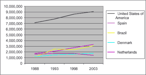
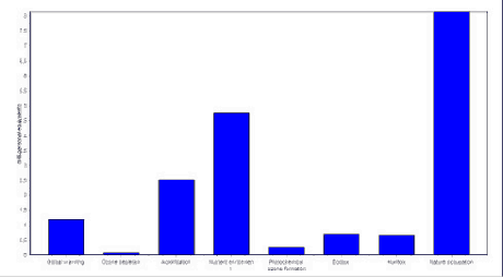
Figure A.1. Development in Pig Production 1088-2003 in the 5 countries under study (in Mg) (FAOSTAT 2004).

The pig production in US, Spain and Brazil is increasing rapidly (see figure A.1), whereas the production in Denmark experiences a more modest growth. Pig production in the Netherlands is stable/slightly decreasing.

A.2 What do we know about environmental impacts from pig production?

The LCAfood project (Nielsen et al., 2003) provided a database for environmental assessment of basic food. In this model, Danish pig production is split up into 7 farm types according to animal density and soil type. The most important inputs and outputs as well as emissions to air and water from these productions are modelled according to national statistics.

As can be seen in figure A.2, the main environmental impacts from Danish pigs are nature occupation and nutrient enrichment, when assessed with the EDIP impact assessment methodology extended the impact category nature occupation (as a rough indicator for biodiversity impacts of land use).

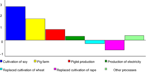
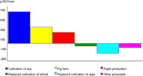
Figure A.2. Normalised environmental impact from 100 kg Danish pig.Calculation based on data from Nielsen et al. (2003) and EDIP impact assessment methodology, adapted by Nielsen et al. (2003).

Nature occupation is the environmental impact category contributing most to the normalised score. Approximately 50 % of the land use contributing to nature occupation is caused by production of soy, which is used as protein feed input in the pig production.

Nutrient enrichment is mostly caused by nitrate and ammonia from agricultural productions. Less than 1 % comes from combustion processes in agriculture, transport and other production.

Acidification is almost entirely caused by ammonia from pig production.

Nitrous oxides and methane from agricultural productions make up 80 % of the global warming, whereas CO2 only contribute 20 %.

Note that pesticides are not included in this assessment, and the impact categories ecological toxicity and human toxicity mainly cover toxic impacts from combustion processes.

For eutrophication, global warming, and nature occupation, the main contributions are from the production of pigs at the farm and the soybean cultivation, see figures A.3-A.5. In these figures, the pig production is modelled as a pig farm including fattening of pigs (from 30 kg to 100 kg) and cultivation of various crops at the associated farmland. Production of piglets (breeding and fattening till 30 kg) is assumed separated from this production. Soy cultivation abroad supplies protein feed for the production. Note that transportation of soy to Denmark and processing into livestock feed contributes insignificantly to the environmental impacts. All environmental impacts at the farm are attributed to the pigs, which are considered the main product determining the overall production. The crop by-products produced at the pig farm are assumed to replace similar productions elsewhere in the world. The emissions and use of resources from these replaced productions thus contribute with negative environmental impacts (seen as the negative values in figure A.3-A.5).

Figure A.3. Contribution to global warming from 1 kg Danish pig ready for slaughter divided on processes. Processes contributing with more than 5 % of the total amount are shown individually. Calculation based on Nielsen et al. 2003.

Figure A.4. Contribution to Eutrophication from 1 kg Danish pig ready for slaughter divided on processes. Processes contributing with more than 5 % of the total amount are shown individually. Calculation based on Nielsen et al. 2003.

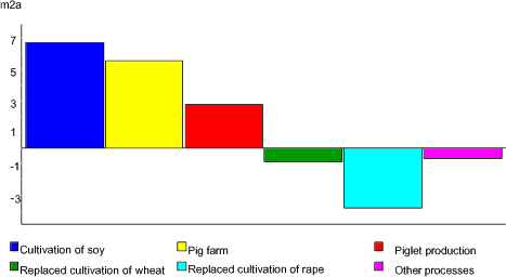
Figure A.5. Contribution to nature occupation from 1 kg Danish pig ready for slaughter divided on processes. Processes contributing with more than 5 % of the total amount are shown individually. Calculation based on Nielsen et al. 2003.

A.3 Scope of the data collection of this study

Based on the knowledge of the Danish farm system and its main environmental impacts, as outlined above, we concentrated the data collection for the foreign competing products on the following data:

• Feed consumption and composition for piglet production and fattening, and the consequent feed production emissions and land use.
• Emissions from piglet production and fattening of pigs, and the related manure handling, with special focus on the substances contributing to global warming (N₂O, CH₄ and CO2), acidification (NH₃) and eutrophication (evaporation of NH₃, potential leaching of nitrogen from arable land where manure is supplied).
• Data from the slaughtering process.

Data are collected for the modern production technology, which is likely to be implemented to meet future increases in demand. Pig production is modelled separately from cultivation of crops.

A.4 Description of production technology

All 5 countries have experienced the same development towards industrialised production.

In this development, pig production has been separated from other agricultural productions, which also means that feed production (crop cultivation) and utilisation of manure as fertiliser in crop cultivation are now increasingly separated.

In US, parts of the administration and marketing have been split out from pig production as well. The majority of US pigs are thus produced on farms that are run by a farmer (operator) different from their owner (contractor), a trend also seen in Spain.

Pig production units have grown in size. For example from 1982 to 1997 in US, the number of pigs per farm increased by more than 300%, while the number of pig farms decreased by two thirds (McBride, 2003).

Newest development goes in the direction of further specialisation, where the processes of farrowing, nursing and fattening are split out on separate production units.

A.4.1. Manure handling systems

Manure used to be utilised as fertiliser in crop production. With the above-mentioned development of pig production, all countries face the problem that manure is in excess on pig producing farms. Artificial fertiliser is relatively cheap compared to the cost of storing and transporting manure to distant crop producing areas.

In Europe, much focus has been on the negative impacts of nutrient enrichment caused by emissions from manure.

In Netherlands as well as Denmark, manure is always stored in covered tanks, which is the storage system with the lowest emissions. In Spain, some open storage may still exist, but the marginal production (i.e. the new production units that are installed with increasing production) will have modern technology with covered tanks. When manure is applied as fertiliser on land, emissions are highest when manure is applied with a sprinkler, and lower when the manure is incorporated into the soil.

In contrast, a combination of lagoon storage and sprinkler application is actively used in US to increase evaporation (emissions to air) and decrease emissions direct to water biotopes.

Only approximately 80 % of the small farm units have a manure storing facility (see table A.2.). The remaining farms must be assumed to use the storing system of neighbouring farms or apply manure on farmland immediately.

Modern productions always have manure-storing systems. In the southern seaboard (North Carolina), use of lagoons is absolutely prevalent. In the US heartland (Iowa), more than 30 % is stored in pits or tanks. This can be explained by the bigger amount of crop production in the heartland, which makes it more economically interesting to utilise manure as fertiliser. Also, application of manure by incorporation into the soil (either by injection or tillage operation) is much higher in the heartland, than in the southern seaboard. More than two-thirds of the liquid manure from medium or large-scale production operations in the Heartland was incorporated into the soil (either by injection or tillage operation) at application, compared with less than 15 percent of manure on those operations in the southern seaboard (McBride, 2003).

A major part of the growth in US pig production can be expected to take place in North Carolina (McBride, 2003). Therefore storage of manure in open lagoons is assumed for the modelling.

Table A.2. Presence of manure storing facilities at farms in US (McBride, 2003). i.d. means insufficient data. 1 Animal unit equals 7.8 pigs raised from 20 to 100 kg. Further definition of this term can be found in table D.7.

Data from Brazil report of manure stored in grooves covered with plastic or masonry.

A.4.2. Feed efficiency

The feed conversion factor, or feed transition coefficient is the amount needed of kg feed to produce 1 kg pig ready for slaughter. It is usually calculated separately for the breeding, piglet production and the fattening period (see table A.3). However, it is usually only the feed conversion factor in the fattening production that is compared (see e.g. table A.4), since in the piglet production the crucial parameter is rather the number of piglets per year-sow.

Table A.3. Feed conversion factors in Danish pig production.

Table A.4. Average feed conversion factors for the fattening period (Rasmussen, 2004).

The average feed conversion factors estimated by the Danish National Committee of Pig Production (table A.4) are not necessarily representative of the modern technologies, which will be affected by future increase in demand. In general, in our own data-collection (see tables A.5-8) we have not found any significant difference in feed conversion factors for fattening between modern, industrial scale farms in the different countries. This implies that the only difference in the overall feed conversion factors (i.e. including the breeding) is due to the difference in number of surviving pigs per year-sow (see table A.9).

Table A.5. Feed conversion factors in Dutch farms. DSU meansDutch Size Units and is a measure of the economic size of agricultural productions based on the standard gross margins.

¹ Data from Rasmussen (2004). 2 Data from LEI (2004).

National statistics on Dutch pig production shows that the feed conversion factor does not vary significantly between farm sizes (see table A.9). Integrated farms have a slightly lower feed efficiency than farms specialised in production of either piglets or fattening pigs.

Table A.6. Feed conversion factors for modern technology in Spain. All data are in kg feed per kg weight gain. Data from database of private consultancy, see annex C, section 1.2.

Table A.7. Feed conversion factors for 4 different sizes of pig production in US. All data are in kg feed per kg weight gain. Source: McBride (2003; table 6).

* uncertainty on this estimate is higher than on other estimates in this table (coefficient of variation between 25 and 50).

nr indicates not reported due to a limited sample size and a high coefficient of variation.

Data in table A.7 cover average US production grouped according to type of production as well as size. Industrial productions always have the lowest feed coefficients. The relatively high values for integrated farms may be explained by the fact that they are often older farms.

Table A.8. Feed conversion factor for production units in three areas of USA. McBride (2003). All data are in kg feed per kg weight gain.

1 uncertainty on this estimate is higher than on other estimates in this table (coefficient of variation is higher than 50). nr indicates not reported due to a limited sample size and a high coefficient of variation.

Table A.8 shows average US productions grouped according to geographic location and type of production. The relatively low values for production in the Southern Seaboard can be explained by the recent production increases in this area, which implicates that the estimate in table A.8 cover a larger share of modern farms. The estimates for disintegrated production in the Southern Seaboard could therefore be used as estimate of modern US technology.

For Brazil a value of 2.5 kg feed per kg pig was reported. However, this was not verified from other sources.

We have not found any convincing arguments to support that the feed transition coefficient for fattening in modern, industrialised technology should vary between the countries. However, taking to account the differences in number of pigs per sow, the overall feed conversion factor does vary slightly between the countries as seen in Table A.9.

Table A.9. Number of pigs per year-sow and overall feed conversion factors for modern, industrialised farms in the five countries.

1) Rasmussen (2003)
2) In feed units per kg weight gain

A.4.3 Feed composition

Carbohydrate crops such as maize, cereals (barley, wheat, etc.) form the energy basis of the feed. This may be substituted to some degree by industrial by-products when available. However, this availability is limited by the production volume of the corresponding main products. Therefore, an increase in pig production cannot be based on industrial by-products, and the standard feed rations we have used in our calculations are therefore based exclusively on crops.

In Denmark and the Netherlands, barley and wheat/triticale are the most important sources of carbohydrate, whereas maize is the major feed input in US. In Spain a combination of maize and cereals is used.

The typical protein source is soy meal from soybeans. USA, Brazil, Argentina and Canada supply the majority of soybeans. In Spain, spring peas is reported as a competitive national ingredient that allows a reduction in price and therefore is used whenever available. However, the significant amount of the protein feed for pig production in all countries can be expected to come from soy meal.

Based on data on feed combinations in the different countries in table B.1, C.2, D.1 and D.4, the marginal feed combinations in table A.10 are used for our comparisons. For Spain we assume that modern productions will have the same relationship between protein and carbohydrate feed as Danish and Dutch productions. For US, we have assumed a relatively high-protein feed combination to be representative of the marginal production facilities. For Brazil, the input of meat meal has been converted to soybean meal in the marginal feed combination.

Table A.10. Marginal feed combinations in pig production (in mass-%)

Based on the data presented above, a model for each production is compiled in the table below. Inputs of crop based live stock feed and synthetic amino acids are estimated based on a the feed coefficients in table A.9 and the feed combinations in table A.10. A supplement of synthetic amino acids and mineral feed is estimated based on Danish data.

Table A.11. Feedstuff inputs to pig production.

The data are chosen to reflect the technology that will be used for future production increases, i.e. specialized, large-scale production.

Soy is traded on a global market. Increases in consumption of protein feed will most likely affect the production of soybean in South America, no matter in which country the consumption takes place. Therefore a common cultivation model for South American soybean (from Nielsen et al. 2003) has been used for calculating environmental impacts from all 5 countries.

Similarly, wheat and other carbohydrate feed stuffs are traded on more regional markets, but changes in consumption in one part of the world may still influence production in another part. Therefore we have used a common cultivation model for wheat and barley (from Nielsen et al. 2003) to estimate the environmental impacts from the consumption of carbohydrate feed. Emissions from maize cultivation has been modelled as equal to those from cultivation of the same quantity of wheat, but the land use adjusted to a yield of 9 Mg per ha.

A.5 Inputs of energy in pig production

Energy is used for transport and handling of manure and for heating and light in the production plant etc.

The Dutch estimate of energy consumption is shown in table A.12. Energy consumption is highest in the breeding phase. Differences in energy consumption in the farms sorted by size can be explained by differences in the amount of breeding and piglet production.

Table A.12. Direct use of energy per fuel on Dutch farms (stables only). All Data in MJ/kg produced pig.

Danish data are in the same range as the Dutch, but in the statistical data it is less easy to distinguish between energy used in stables and energy used for other farm processes.

The Spanish data have been discarded, as they were conspicuously low in comparison. Based on Ozkan and Harmon (1995), the American fuel consumption can be estimated to 3.0 MJ/kg pig. These data are, however, quite old.

Because of the low importance of the energy consumption for the overall impact from pig production, no particular effort has been spent on improving the data quality. In the calculations, we therefore use the same data (for the Dutch production on integrated farms for all countries (i.e. 2.34 MJ diesel and 0.8 MJ direct electricity).

A.6 Emissions to air from pig production

Emission from the manure depend upon the manure handling system and the climate, and is identified as one of the most important differences between the production systems in the different countries. Air emissions increase by high temperatures storage in open pits or lagoons instead of covered tanks, application by use of sprinkler instead of incorporation into the soil, and high temperatures.

A.6.1. Emissions of NH₃

In the table below, the average data on emission of ammonia from pig production is presented.

Table A.13. Emission of ammonia from pig production per kg produced pig, average technology. All figures in g N/kg pig. Values have been rounded.

1) Hutchings et al. (2001). 2) Own calculation Based on Hoek (2002) and Statistics Netherlands (2004). 3) Own calculation Based on closed-cycle production systems cf. Spanish Ministry of Agriculture, Fisheries and Food. (2004). See further details in Table C.4. 4) Own calculation Based on US EPA (2004).

The values in table A.13 refer to average production. Danish and Dutch values were not found to vary significantly. No specific data were found for Brazil. Since the manure storage conditions appear to be closer to European, and the climate of Brazil is closer to Spain than to Denmark or The Netherlands, the Spanish data are used as a proxy for Brazilian data.

Modern production units can be expected to have a lower amount of nitrogen in the manure as a consequence of the lower feed transition coefficients. In table A.14, the above data are adjusted in accordance with the feed inputs of the modern technology farms, as outlined in Chapter A.4.

For Spain, further details on the emission factors are presented in table C.4. For USA, the data represent the production system of the South-eastern seaboard, where the focus is on minimising eutrophication of water by maximising emissions to air.

Table A.14. Emission of ammonia from pig production per kg produced pig, modern technology. N in manure is own calculation based on the use of feed presented in Chapter A.4. All figures in g N/kg pig. Values have been rounded.

A.6.2. Emissions of methane

Given the very similar feed conversion factors between the countries, the difference in methane emissions (which are calculated with standard factors based on the feed input) is also limited. Calculated with the default methane conversion factor provided by IPCC (39%) the emission is 65 g CH₄/kg pig for DK, NL and Brazil, and 66g CH₄/kg pig for ES and USA.

A.6.3. Emissions of N₂O

Emissions of nitrous oxides from pig production are estimated on the basis of the nitrogen balance of the production (see table A.17) and standard emission factors: the emission of nitrous oxides is estimated to be 1 % of the nitrogen emitted as ammonia, and 2.5 % of the nitrogen potential for leaching.

Table A.15. Estimates of emissions of nitrous oxide from pig production. All values in g N₂O per kg pig.

A.7 Emissions to water from pig production

Potential leaching of nitrogen are calculated based on nutrient balances.

The emission data presented in the previous sections are integrated with the data on feed consumption and modified to give a realistic model of the substance flows of the pig production.

Emissions to water can be estimated as the difference between nutrients in the inputs (feedstuffs) minus the outputs in pigs, crops and known emissions.

To calculate the nutrient content of the inputs, the data presented in the table below have been used.

Table A.16. Content of dry matter and nitrogen in feedstuff. (Møller et al. 2000 og Landsudvalget for svin 1994).

Based on table A.16 and the adjusted data on feed consumption and emissions, the nutrient balance is calculated in table A.17. The amounts of N utilised by plants have been estimated to 50% of the available N, except for Denmark where legislative requirements have raised this to 75%.

Table A.17. Nitrogen balance of pig productions. All data in g N per kg produced pig. Nitrogen content in feed is calculated from the feed inputs in table A.11 and the nutrient contents of table A.16. Differences in sums due to rounding.

A.8 Avoided emissions from artificial fertiliser

The N utilised by plants from Table A.17 is calculated as avoided artificial fertiliser input, using the data from LCA-Food (Nielsen et al. 2003), which includes production of artificial fertiliser, the difference in energy for spreading, and field emissions related to application of artificial fertiliser.

A.9 data uncertainty

Uncertainties on the above data sources have been estimated and are summarized in Table A.18.

Table A.18. Uncertainty estimates for the data applied in this analysis

Uncertainty on the feed coefficient is used as uncertainty factor for the single feed inputs, which also affects the area occupation. For Denmark, the Netherlands and Spain these values are estimated based on table A.5. Uncertainties for US and Brazil are estimated based on table A.8. Since data in these tables reflect average technology, we assume that the uncertainty is lower in the fraction representing modern technology. Because of the lack of specific data for Brazil, the higher value is chosen.

The uncertainties on the methane emissions are estimated from the uncertainty in feed coefficient, since methane emissions relate to the amount of dry matter in manure, which again depends upon the amount of feed.

For US, uncertainty on all nitrogen-related emissions and on the amount of replaced artificial fertiliser has been estimated from model calculation of 3 scenarios with different manure handling systems: 1) maximum evaporation from the manure lagoons, 2) Dutch manure handling technology, and 3) an average situation where 30 % of the N-surplus in manure is lost from the lagoons as ammonia, and 14 % of the N-surplus in manure ex storage is lost as ammonia from field application with sprinkler system.

For all other countries, the uncertainty of the ammonia emission is estimated from uncertainty on feed coefficient (see above) plus an extra uncertainty caused by differences in manure handling.

The amount of fertiliser, which can be replaced by pig manure, is fixed by regulation in Denmark. Therefore the uncertainty on this value is estimated based on the uncertainty of the feed intake. For the Netherlands, Spain and Brazil the uncertainty is based on results from field-experiments of the fertilising effect of manure.

Nitrate emission to water (N-tot) is closely connected to the amount of nitrate taken up by the plants, and therefore we estimate the uncertainty to be similar to the uncertainty of the amount of replaced fertiliser (see above).

Emissions of nitrous oxides depend partly upon the emissions of ammonia, partly on the emission of nitrogen to water. Therefore the uncertainty is estimated as the larger uncertainty of these variables.

References

McBride W D, Key N. (2003). Economic and Structural Relationships in U.S. Hog Production. Agricultural Economic Report No. 818. U.S. Department of Agriculture. Resource Economics Division, Economic Research Service.

Hauschild M, Potting J. (2004). Spatial differentiation in life cycle impact assessment – the EDIP2003 methodology - Final Draft. Guidelines from the Danish Environmental Protection Agency. Copenhagen: Danish Environmental Protection Agency.

van der Hoek KW. (2002). Input variables for manure and ammonia data in the Environmental Balance 1999 and 2000. RIVM Rapport 773004012. In Dutch. http://www.rivm.nl/bibliotheek/rapporten/773004012.html.

Hutchings N, Sommer S G, Andersen J M, Asman W A H. 2001. A detailed ammonia emmision inventory for Denmark. Atmospheric Environment 35:1959-1968.

Landsudvalget for svin (1994). Foderstoffer til svin.

LEI (the agricultural economics research institute of Netherland), 2004. Binternet statistics. Available at http://www2.lei.dlo.nl/binternet. Accessed April 2004.

Møller J, Thøgersen R, Kjeldsen A M, Weisbjerg M R, Søegaard K, Hvelplund T, Børsting C F. (2000). Fodermiddeltabel. Rapport nr. 91, 1-52.

Mount R, Zelling K D, Stanislaw C M. (1994). Production and financial summary - 1993. North Carolina State University. Swine development center. Available at http://mark.asci.ncsu.edu/ECONOM~1/pf_sum93.htm.

Nielsen P H, Nielsen A M, Weidema B P, Dalgaard R, Halberg N (2003). LCA food data base. www.lcafood.dk.

Ozkan E, Harmon J. (1995). Estimating farm fuel requirements for crop production and livestock operations. Iowa State University, Department of Agricultural and Biosystems Engineering. http://www.abe.iastate.edu/livestock/pm587.asp.

Rasmussen J. (2004). Costs in international pig production 2002. Report no. 24. Denmark: the National Committee for Pig Production.

Spanish Ministry of Agriculture, Fisheries and Food. (2004). Ganaderia. Emisiones de Gases en la Ganaderia. Available through http://www.mapya.es/es/ganaderia/pags/Emisiones_gases/emisiones.htm

Statistics Netherlands. (2004). Milieu, natuur en ruimte. Dierlijke mest en mineralen 2001. Available at http://www.cbs.nl/nl/publicaties/artikelen/milieu-en-bodemgebruik/Milieu/mest/2001/dierlijke-mest-mineralen-2001.htm

US EPA. (2004). Unspecified statistics.

Western Area Power Administration. (2004). Technical Help. Accessed October 2004 at http://www.wapa.gov/es/techhelp/powerline/98sep.htm.

| Forside | | Indhold | | Forrige | | Næste | | Top |

Version 1.0 August 2005, © Miljøstyrelsen.