Environmental Project No. 1296, 2009
Model assessment of reductive dechlorination as a remediation technology for contaminant sources in fractured clay: Case studies
Delrapport III
Contents
2 Modeling and remediation objectives
- 4.1 Characterization of contamination source
- 4.2 Geological characterization – Fracture distribution
- 4.3 Hydrogeological characterization
- 4.4 Model configurations and scenarios
- 4.5 Modeling results
- 4.6 Sensitivity analysis on parameters
- 5.1 Characterization of the contaminant source
- 5.2 Geological characterization – Fractures distribution
- 5.3 Hydrogeological characterization
- 5.4 Enhanced reductive dechlorination
- 5.5 Model configuration and scenarios
- 5.6 Model results
- 6.1 Characterization of contamination source
- 6.2 Hydrogeological characterization
- 6.3 Use of EPM model
- 6.4 Enhanced reductive dechlorination
- 6.5 Model configuration and scenarios
- 6.6 Model results
- 7.1 Comparison between the sites
- 7.2 Recommendations for definition of remediation criteria
- 7.3 Recommendations for field investigations prior to and during remediation
- 7.4 Recommendations for use of reductive anaerobic dechlorination
- 7.5 Recommendations for improving modeling tool
Preface
Enhanced reductive dechlorination has successfully been applied in high permeability media contaminated with chlorinated ethenes, but has not yet proved its effectiveness for use in low permeability media. In Denmark there are only few examples of such “in-situ” bioremediation, focusing on the source zone located in clay till and so there is a need for a better understanding of the different processes implied in this remediation technology.
The first and second phases of this project consisted in gathering the different experiences for reductive dechlorination as a remediation technology in clay till in Denmark and developing a modeling tool for assessing efficiency and time horizons for enhanced reductive dechlorination in clayey till. This report is the third phase of the project, where the developed model is applied to three Danish sites with chlorinated solvents in clayey till, where enhanced reductive dechlorination has been either applied or considered as a remediation technology.
The project is financed by Region Hovedstaden and Miljøstyrelsens Teknologiprogram for jord- og grundvandsforurening.
Miljøstyrelsen has appointed a management group in order to follow the work. The group consists in:
- Carsten Bagge Jensen, Region Hovedstaden
- Henriette Kerrn-Jespersen, Region Hovedstaden
- Jesper Elkjær, Region Hovedstaden, now in Københavns Energi
- John Flyvbjerg, Region Hovedstaden
- Ole Kiilerich, Miljøstyrelsen
- Mette Christophersen, Region Syddanmark
- Henrik Rud Larsen, Region Midtjylland
1 Introduction
1.1 Background
Chlorinated solvents are wide spread subsurface contaminants and an important threat to groundwater quality. Chlorinated solvents are sparingly soluble dense non aqueous phase liquids (DNAPL) that can be long term sources of contamination to groundwater. Many contaminated sites occur in areas with fractured clay geology at the land surface (Chapman and Parker 2005), where the released DNAPLs penetrate into preferential flow pathways formed by fractures and can then rapidly dissolve and diffuse from the fractures into the matrix (Falta 2005). Even after the removal of the physical source from the site, the contaminant can back diffuse to the fracture network for hundreds of years, causing long-term contamination of an underlying aquifer (Harrison et al. 1992,Parker et al. 1997,Reynolds and Kueper 2002). In Denmark, clay tills are wide spread and this scenario is very common. It is important to characterize the behavior of chlorinated solvents sources in clay aquitards so as to be able to predict their impact on the underlying groundwater aquifers. The remediation of contaminated clayey till sites is very challenging, because of the complexity of the source, the processes taking place and the mass transfer limitations due to slow diffusion process in the low permeability clay matrix (Johnson et al. 1989).
Recent laboratory and field experiments have shown that bioremediation may be an attractive method for chlorinated solvents decontamination. Chlorinated solvents can be anaerobically degraded through sequential reactions to a non toxic end product (ethene). These sequential reactions are termed “reductive dechlorination”. This degradation is possible in an anaerobic environment, with the presence of both dechlorinating bacteria and electron donor (generally hydrogen).
Bioremediation, where an electron donor and/or bacteria are injected into the fracture system to enhance reductive dechlorination, is a promising remediation technology that may be able to reduce clean-up times.
1.2 Project description
The overall purpose of the project is to assess the effects and timeframes for remediation using enhanced reductive dechlorination in clay till. The first phase consists in gathering the different experiences for reductive dechlorination as a remediation technology in clay till in Denmark (Miljøstyrelsen 2008b). A modeling tool for assessment of the time horizons for remediation of low permeability media using reductive dechlorination has been developed during the second phase (Miljøstyrelsen 2008a).
In this third phase, the modeling tool is tested on three selected case sites each representing clay till systems with different occurrences of vertical fractures, horizontal sand lenses and sand stringers.
The initial model presented in (Miljøstyrelsen 2008a) has been further developed and Section 3 gives a short description of the model and the new features.
2 Modeling and remediation objectives
2.1 Aim of modeling
The overall purpose of the modeling tool is to assess the performance of enhanced reductive dechlorination (ERD) as a remedy for contaminated low permeability media.
For each of the test sites, the model will be used to provide information on the temporal development of three important performance metrics:
- residual source mass
- contaminant mass flux out of the source zone
- average source zone concentrations
The performance metrics will be evaluated for a number of different remediation scenarios representing different situations in terms of distribution of bacteria and substrate in the subsurface. The remediation scenarios will be compared to a baseline scenario without enhanced dechlorination.
The model consists of two components: a model of the fractured clay system containing the contaminant source; and a model of the underlying groundwater aquifer. The contaminant flux from the fractured clay source model is input to the aquifer model in order to estimate the expected aquifer concentrations in either a upper or regional aquifer depending on the remediation objectives for the specific site.
Given the remedial objectives for a site, the model is used to assess the timeframe for achieving the desired cleanup level. This requires that a clear and operational termination criterion for the site cleanup has been set, which is not always the case in real life applications (Miljøstyrelsen 2008b).
To address parameter uncertainty, a number of sensitivity scenarios will be presented for one of the sites. In the sensitivity analysis, the sensitivity of the various parameters e.g. fracture spacing and degradation rates is assessed by examining the effect on the calculated mass removal and contaminant flux.
2.2 Remedial objectives
Remedial objectives must be defined before commencing treatment of contaminant sources such as clay till source zones.
The task is not as straightforward as it is for groundwater plumes in aquifers, where compliance with groundwater quality criteria can directly be used as a remedial objective. In-situ remediation of clay till source zones eventually results in compliance with objectives of groundwater quality, but as there is a delay before an aquifer experiences the impact of source zone remediation, groundwater cleanup criteria are less useful for determining when a source zone treatment can be terminated.
In the following section a framework for setting of remedial objectives is presented. This is followed by a presentation of the existing remedial objectives for the three case studies used in this report.
2.2.1 Absolute objectives and functional objectives
Following the nomenclature of ITRC (ITRC 2008), remedial objectives can be either absolute or functional. Absolute objectives describe the overall goals of remediation and represent social values such as protection of human- or ecosystem health and preventing deterioration of groundwater resources. Each absolute objective should be accompanied by a number of functional objectives that are means by which the absolute objective is achieved. A functional objective should be equipped with a quantifiable performance metric which can readily be measured; alternatively the functional objective can be broken down into subsidiary measurable objectives.
As an example, consider a contaminated site with an absolute objective of protecting the groundwater resource. The contaminant source is located in a low permeability clayey till overlying a groundwater aquifer used for drinking water extraction. An upper aquifer not used for drinking water extraction is also present. The conceptual site model is presented in Figure 2.1.
A common functional objective for such a site is the compliance with groundwater quality criteria at a certain point of compliance. Possible points of compliance are: (a) the upper aquifer at the downstream boundary of the treatment zone; (b) the regional aquifer at the downstream boundary of the treatment zone; and (c) the regional aquifer at a downstream receptor (drinking water well, receiving water body).
Figure 2.1 - Conceptual site model for setting of remedial objectives. Possible locations for point of compliance (POC) with groundwater quality criteria are indicated.
Since source zone remediation does not affect groundwater concentrations immediately, quality criteria cannot be used directly to guide the remedial action taken in the source zone. In order to have an operational termination criterion it is therefore necessary to define a subsidiary functional objective for the source zone, where the effect of remediation is monitored.
Thus we will advocate for the use of two complementary functional objectives in the case of source zone remediation:
- Long term functional objective: To comply with groundwater quality criteria at selected point of compliance in the groundwater. Performance metric: groundwater concentration (µg/L).
- Source zone functional objective: To reduce the source zone contamination to a level that ensures that the long term functional objective is met. Performance metrics: total[1] soil concentrations in source zone (mg/kg), source zone aqueous concentrations (µg/L), and contaminant mass flux from source zone (kg/yr).
Objective 2 can be seen as a termination criterion for the source zone treatment, whereas objective 1 is a termination criterion for the post-remediation monitoring.
Setting of a source zone termination criterion requires that modeling of the contaminant attenuation from the source zone to the chosen point of compliance is carried out.
The termination criterion for the source zone is ideally defined in terms of the total (or percentage) mass removal, as this is a more reliable metric than aqueous concentrations when it comes to assessing the extent of residual contamination left in the source zone. Continuous monitoring via soil cores is not typically conducted during site remediation as it is more practical and economically feasible to monitor via water sampling. A termination criterion expressed in terms of aqueous contaminant concentrations in the source zone, should preferably be accompanied by a total soil concentration criterion. When the termination criterion for the aqueous phase has been achieved, the next step is to investigate the compliance with a termination criterion defined by total soil concentrations.
Another possible performance metric for defining a termination criterion is the total contaminant mass flux leaving the source zone. This definition requires that a procedure for determining the site-specific mass flux is available i.e. via multilevel sampling along a cross-section directly downstream the source zone.
Prior to the commencement of the remediation, it is essential to establish a baseline for each of the performance metrics used (contaminant mass in source zone, total contaminant concentrations in source zone, contaminant mass flux from the source zone). This makes it possible to evaluate the changes in the contaminant situation at the site.
2.2.2 Remedial objectives at Vadsbyvej
A conceptual sketch of the Vadsbyvej site is presented in Figure 2.2. In the risk assessment for Vadsbyvej (Region Hovedstaden 2008c) the absolute objective of a remedial action at the site is defined to be the protection of the groundwater resource to ensure its future use as a source of drinking water. There are no risks related to the present land use and no surface water receptors at risk.
Figure 2.2 – Conceptual sketch of the Vadsbyvej site. The remediation objective for the site is based on complying with quality criteria in the abstracted drinking water at the water supply well 500 m downstream from the site.
The risk assessment concludes that at present there is no acute risk of contamination of the drinking water abstracted at the nearby well field. Based on the elevated contaminant concentrations in the source zones it is, however, anticipated that there will be a significant risk in the future. As the upper sandy aquifer is hydraulically connected to the regional aquifer in the downstream direction, the two aquifers are regarded as one interconnected aquifer in the risk assessment.
A long term functional objective is defined as complying with the drinking water quality criteria for the groundwater abstracted at the downstream water supply. Based on this long term objective, a criterion for the short term has been defined as the maximum mass flux in the upper sand aquifer that satisfies the long term criterion. This is combined with a criterion for the maximum concentration of vinyl chloride in the sand aquifer. Thus the two short term functional criteria that in combination define the termination criteria for a successful remediation are (Region Hovedstaden 2008c):
- to obtain a stationary or decreasing contaminant flux in the upper sand aquifer compared to the baseline of 10 g/year (sum of chlorinated solvents: chlorinated ethenes and ethanes, ethene/ethanes are not included in this sum)
- to obtain a stationary or decreasing concentration of vinyl chloride in the upper sand aquifer compared to the baseline of 60 µg/l.
These objectives are irrespective of the choice of technology for remediation. Furthermore a temporary increase in both contaminant flux and concentrations can be accepted during treatment (Region Hovedstaden 2008c).
The baseline flux was estimated from (a) a volume pumping of a well downstream from the hotspots and (b) a mass flux calculation based on contaminant concentrations in four wells and assignment of a representative cross-section area to each well. A homogenous flow field (hydraulic conductivity and gradient) in the upper aquifer was assumed and the hydraulic conductivity was estimated using pump test data.
The existing remedial objectives for Vadsbyvej can be used together with the models to assess the time horizon for cleanup. However, as the modeling tool only handles chlorinated ethenes and not chlorinated ethanes, the flux criterion is reduced to only represent the contaminant flux of chlorinated ethenes which according to the flux calculations in (Region Hovedstaden 2007) constitutes approximately 20% of the total contaminant flux from the site. The existing termination criteria could be strengthened by combining it with a criterion considering the total soil concentration in the source zone.
2.2.3 Remedial objectives at Gl. Kongevej
As for Vadsbyvej, the absolute objective of remediation is to protect the drinking water aquifer. The drinking water aquifer at Gl. Kongevej is approximately located only 9 meters below the surface and has already been significantly contaminated. A sketch of the Gl.Kongevej site is seen in Figure 2.3. In 2004 it was suggested that the contaminant flux from the source zone was to be reduced by a factor of 100 as concentrations of up to 70 µg/L (sum of chlorinated ethenes) was found in the regional groundwater. In addition to this, a termination criterion of 10 µg/L (sum of chlorinated ethenes) in the source zone porewater was suggested (Miljøkontrollen 2004a).
Later investigations measured concentrations of up to 3100 µg/L (sum of chlorinated ethenes) in the drinking aquifer (Miljøkontrollen 2005). In 2006, in-situ stimulated reductive dechlorination was initiated at the site and a number of revised functional objectives were formulated (Miljøkontrollen 2006). A short term functional objective was set to be the achievement of stationary or decreasing concentrations (and flux) of chlorinated ethenes in the drinking water aquifer within 5 years from initiation of the treatment. An actual termination criterion was suggested to be the reduction of concentration levels in the treatment zone with a factor of 50 as this would give an equivalent reduction in the contaminant flux to the aquifer.
As this termination criterion is a rough estimation we will investigate the necessary cleanup level further by using the modeling tool. Hence for the purpose of the performance modeling in this report, a functional objective of complying with groundwater quality criteria is used and a point of compliance is chosen at the downstream boundary of the treatment zone in the drinking water aquifer (POC (b) in Figure 2.3). A termination criterion for the source zone is then assessed by a combined use of a source zone flux model and an aquifer model.
Figure 2.3 - Conceptual sketch of the Gl. Kongevej site. The proposed long term remediation objective is to comply with quality criteria in the regional aquifer at the downstream boundary of the treatment zone. The treatment zone is indicated with the dotted black box.
2.2.4 Remedial objectives at Sortebrovej
At the Sortebrovej the source zone is located in at clayey till layer overlying an upper aquifer, which is also significantly contaminated (see Figure 2.4). The clayey till source zone has a significant number of sand lenses and -stringers from which groundwater is monitored during remediation. The absolute objective at Sortebrovej is to protect the groundwater resource. As for Gl. Kongevej a short term objective is to achieve stationary or reduced concentration levels of chlorinated solvents in the regional aquifer within 5 years of the start of remediation (Fyns Amt 2006a). A termination criterion was initially suggested to be the reduction of source zone concentrations with a factor of 50-100 (Fyns Amt 2006a). The remediation objectives for Sortebrovej were revised and further specified in 2008. The long term functional objective is defined as to comply with groundwater quality criteria at a point of compliance in the regional groundwater at the downstream boundary of treatment zone (Region Syddanmark 2008a). As the effect on the aquifer is delayed in time, this long term objective is combined with a termination criterion based on source zone concentrations. The criterion for termination of the treatment is to reduce the average aqueous concentrations in the high permeable structures in clay till source zone to 100 µg/L (sum of chlorinated ethenes). The baseline concentration level in this aquifer was found to be 11 000 µg/L. The compliance with the termination criterion is to be reflected in 3 adjacent monitoring rounds conducted over a minimum of one year to avoid contaminant rebound. The average concentration is evaluated based on 13 monitoring wells screened in the source zone. It is also suggested that soil core sampling is conducted to assess the actual mass removal in the clay till (Region Syddanmark 2008a).
The chosen termination criterion of 100 µg/L for the aqueous source zone concentrations is based on the assumption that the contaminant levels will be reduced by a factor of 100 due to attenuation in the intermediate clay layer and via dilution in the regional aquifer. This assumption will be investigated by expanding the model for Sortebrovej to include the intermediate clay layer and the regional sand aquifer. The termination criterion for the source zone will be revised based on the modeling results.
Figure 2.4 – Conceptual sketch of the Sortebrovej site. The long term remediation objective is to comply with quality criteria in the regional aquifer at the downstream boundary of the treatment zone. The treatment zone is indicated with the dotted black box.
[1] i.e. including contaminant both in the water phase and in the sorbed phase
3 Modeling tool
3.1 Further development of modeling tool
The modeling tool presented in (Miljøstyrelsen 2008a) has been further developed in order to reflect better the reality of the field. The model was taking into account only the fully penetrating vertical fractures and it was assumed that injection of substrate and bacteria was performed in these vertical fractures, allowing a reaction zone to develop vertically around these fractures (Figure 3.2 (left)). However injections at a field site are performed at different interval (called injection depths) and that the injected products are expected to spread horizontally along the natural and/or artificial high permeability features (see Figure 3.1). Therefore the model was further developed to take this phenomenon into account.
Figure 3.1 – Injection and spreading of injected products along high permeability features in the source zone
Figure 3.2 - Development of the modeling tool, from vertical reaction zones around vertical fractures (Delrapport II, (Miljøstyrelsen 2008a)) to horizontal reaction zones around injection depths
3.2 Modeling scenarios
Different model scenarios will be tested for the three sites, corresponding to different spreading of the substrate and biomass into the contaminated clay:
- No dechlorination (baseline) – the system is driven solely by leaching
- Dechlorination at the injection depths only
- Dechlorination in a 10-cm thick reaction zones formed around the injection depths
- Dechlorination in the whole matrix
The background for these scenarios is further explained in (Miljøstyrelsen 2008a), differ.
Figure 3.3 - Illustration of the four different scenarios that were used for the sites
4 Vadsbyvej
- 4.1 Characterization of contamination source
- 4.2 Geological characterization – Fracture distribution
- 4.3 Hydrogeological characterization
- 4.4 Model configurations and scenarios
- 4.5 Modeling results
- 4.6 Sensitivity analysis on parameters
4.1 Characterization of contamination source
The source zone is defined based on the mass distribution calculations performed by the consulting company Orbicon. The concentration measurements performed at the site have shown that the source zone is divided into two hotspots. These hotspots have been further divided into 5 zones each, as illustrated in Figure 4.1.
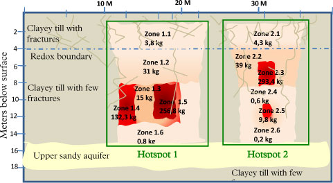
Figure 4.1 - Mass distribution at Vadsbyvej - vertical cross-section adapted from (Region Hovedstaden 2009)
The red zones on Figure 4.1 represent the residual phase, that is assumed to persist at the site. However in the model this residual phase cannot be taken into account. Furthermore the total mass given in the figure has to be converted to aqueous concentrations, in order to be used in the model.
The parameters used for such calculations are taken from (Region Hovedstaden 2008c)
- Clayey till porosity φ = 0.3
- Clayey till bulk density ρb = 1.96 kg/L
The aqueous concentrations are calculated with the following formula:
![]()
Where Cw is the aqueous concentration, Mtot is the total contaminant mass in the zone (without residual phase), Vtot is the total volume of the zone, φ is the porosity, ρb is the bulk density and Kd is the distribution coefficient. Some discussions are currently held concerning the sorption capacity of clay for chlorinated solvents [e.g. (Region Syddanmark 2007)]. Based on experiments conducted at DTU Environment with clay samples from Vadsbyvej and other Danish sites (DTU Environment 2008), the following distribution coefficients for the chlorinated solvents will be used:
- KdPCE = 1.4 L/kg
- KdTCE = 0.6 L/kg
- KdDCE = 0.12 L/kg
- KdVC = 0.04 L/kg
The simplified source distribution is shown on Figure 4.2. At hotspot 2 (zones A2 + B2), PCE is the dominant contaminant and it can be assumed that reductive dechlorination is not taking place. In contrast, hotspot 1 consists of PCE, TCE, DCE and VC in significant quantities, and the presence of daughter products is indicative of reductive dechlorination. This difference between the two hotspots will be taken into account for the modeling.
Figure 4.2 - Simplification of contaminant source distribution and average aqueous concentrations (disregarding the DNAPL phase)
4.2 Geological characterization – Fracture distribution
Intensive field experiments have been conducted at Vadsbyvej on fracture mapping from excavation, but data are available only for the upper 4 meters (above redox boundary). The model of this site is focusing on the zone below the redox boundary. From the field observations and some data extrapolation, a geological model is built for the clayey till, between 4 and 15 meters below surface. This model is based on a linear extrapolation of fracture frequency variation with depth observed at Vadsbyvej (red line on Figure 4.3). Therefore at 15 meters depth, a vertical fracture spacing of 5.6 meters is expected.
Figure 4.3 - Fracture distribution at 13 Danish clay till sites – in red Vadsbyvej (Christiansen and Wood 2006)
It can be assumed that the contaminant has migrated downward from the surface along the vertical fractures. Hence it is expected that the contaminant has spread into the matrix around the fractures. Therefore it is assumed that the two hotspots are each located symmetrically around two of the deepest vertical fractures. This configuration is shown in Figure 4.4.
Figure 4.4 - Vertical fracture network and source location
4.3 Hydrogeological characterization
The hydraulic values (hydraulic conductivities and gradients) for clayey till and the underlying upper sandy aquifer are taken from (Region Hovedstaden 2008c) and summarized in Figure 4.5. These hydraulic conductivities are obtained from slug tests (one in the clayey till at 12 meters depth and two in the sand layer). The vertical hydraulic gradient was assumed based on head measurements in boreholes at different depth in the clay layer. The vertical hydraulic gradient and the bulk hydraulic conductivity correspond to a net recharge rate of 86 mm/year.
Figure 4.5 – Hydraulic characteristics for clayey till and upper sandy aquifer
A water balance can be performed on the source zone sketched on Figure 4.5. Assuming a source width of 22 meters, the water balance can be calculated per unit meter length (see Figure 4.6):
- Vertical water flow through the source zone
Qclay = KbivW = 1.8 m³ / year / m length - Horizontal water flow through the upper sandy aquifer
Qaq = KaqiaqTaq = 1.6 m³ / year / m length
Figure 4.6 – Water balance for the upper sandy aquifer
Assuming that the hydraulic conductivity for the clay matrix is very low compared to Kb (generally in the order of 10-¹0 m/s (Jorgensen et al. 2002)), the average fracture aperture 2b is calculated from the bulk hydraulic conductivity and the spacing between two vertical fractures (2B = 5.6 m) to be 50 µm, with the following formula (Mckay et al. 1993):
![]()
Where ρ is the fluid density (kg/m³), g is the gravitational acceleration (m/s²) and μ is the viscosity (Pa.s).
4.4 Model configurations and scenarios
The model is used to assess the remediation time at Vadsbyvej using enhanced reductive dechlorination for different remediation scenarios, in comparison with the no remediation scenario. The remediation time can be evaluated with respect to the mass removal, the flux reduction and/or the concentration in the upper sandy aquifer. The results from the modeling will be compared with the remediation objectives described in Section 2.2.2.
The geometry (fracture distribution) presented in the previous sections is simplified; the present work focuses on downward transport from the till to the aquifer so horizontal features are neglected. For the same reason, only the fully penetrating vertical fractures are taken into account and an uniform fracture spacing is assumed (see Figure 4.7).
Figure 4.7 - Simplified geometry for Vadsbyvej
The two hotspots are modeled separately in order to reduce model size and computing time.
Different scenarios are considered for the modeling, in order to assess the effect of several remediation strategies compared to applying no remediation:
- Baseline = Reductive dechlorination occurs in hotspot 1, with a reduced amount of specific degraders (measured at the site) and no dechlorination occurs in hotspot 2.
- Remediation A = Reductive dechlorination occurs only at the injection depth.
- A1 - Reductive dechlorination is enhanced with injection of substrate and bacteria every meter
- A2 - Reductive dechlorination is enhanced with injection of substrate and bacteria every 25 cm
- Remediation B = Reductive dechlorination occurs in a 10 cm thick reaction zone around the injection depth (from the results at Rugårsdvej site)
- B1 - Reductive dechlorination is enhanced with injection of substrate and bacteria every meter
- B2 - Reductive dechlorination is enhanced with injection of substrate and bacteria every 25 cm
- Remediation C = Reductive dechlorination is enhanced with injection of substrate and bacteria every 10 cm, and dechlorination occurs in the whole matrix
Figure 4.8 - Schema of remediation A1, A2, B1, B2 and C (from left to right) – the orange areas indicate the location where degradation occurs
4.5 Modeling results
In this section, we will focus on the modeling of hotspot 2, which is the one where reductive dechlorination does not occur naturally. It was decided to focus on this hotspot, as it is estimated that it will take longer to remediate.
4.5.1 Model parameters
Table 1 - Model parameters for Vadsbyvej
| Transport parameters | Value | Reference | |
| Fracture spacing 2B [m] | 5.6 | See Section 4.2 | |
| Fracture aperture 2b [µm] | 50 | See Section 4.3 | |
| Vertical hydraulic gradient Iv [m/m] | 0.2 | (Region Hovedstaden 2008c) | |
| Bulk hydraulic conductivity Kb [m/s] | 1.3*10-8 | ||
| Velocity in fracture vf [m/y] | 9478 | vf = KbI·2B/2b | |
| Matrix porosity φ | 0.3 | (Region Hovedstaden 2008c) | |
| Bulk density ρ [kg/L] | 1.96 | ||
| Tortuosity τ | 0.3 | τ = φ (Parker et al. 1994) | |
| Free diffusion coefficient D*i [m²/y] | (US EPA 2009) | ||
| PCE | 0.018 | ||
| TCE | 0.020 | ||
| DCE | 0.022 | ||
| VC | 0.026 | ||
| ETH | 0.033 | ||
| Sorption coefficient Kdi [L/kg] | See Section 4.1 | ||
| PCE | 1.4 | ||
| TCE | 0.6 | ||
| DCE | 0.12 | ||
| VC | 0.04 | ||
| ETH | 0 | ||
| Dispersivity in fracture [m] | 0.1 | assumed | |
| Microbial parameters | |||
| Maximum growth rate µi [1/d] | |||
| PCE | 3 | Assumed based on (Clapp et al. 2004,Lee et al. 2004) |
|
| TCE | 2 | (Miljøstyrelsen 2008a) | |
| DCE | 0.38 | ||
| VC | 0.14 | ||
| Specific yield Y [cell·µmol/L] | 5.2*108 | ||
| Biomass concentration X [cell/L] | |||
| Natural conditions (hotspot 1) | 107 | ||
| Enhanced dechlorination | 109 | from Gl. Kongevej (Region Hovedstaden 2008a) |
|
The velocity in the fracture can seem very high (9478 m/year), but such high values have been reported in the literature, with velocity up to 9125 m/year in (Mckay et al. 1993), 7800 m/year in (Sudicky and McLaren 1992), between 500-1000 m/year in (Harrar et al. 2007).
4.5.2 Hotspot 2
For hotspot 2, the results of the baseline and the different remediation scenarios are shown in term of both mass removal efficiency (Figure 4.9) and contaminant flux reduction (Figure 4.10).
The mass remaining in the system decreases very slowly for the baseline scenario and that less than half of the initial 40 kg is removed after 2000 years. Concerning the contaminant flux, it is expected to decrease with time from 80 to 25 g/year in 50 years. This simulated flux is higher compared to the measured flux at the site in the upper sandy aquifer (around 20 g/year from both hotspots). Several reasons could explain this difference:
- The initial concentrations in the source are overestimated
- The simulated fully penetrating fractures are not present at the hotspot
- Leaching from the source has occurred during the last 30 years, so the present flux could correspond to the simulated flux at 30 years (equal to 30 g/year)
- The bulk hydraulic conductivity (Kb) and/or the hydraulic vertical gradient (Iv) is overestimated
- The measured contaminant flux in the upper sandy aquifer is uncertain
Remediation scenarios A1 and A2, where dechlorination occurs at the injection depths only neither reduces the leaching time nor the flux compared to baseline scenario. This confirms the conclusions made in (Miljøstyrelsen 2008a); a reaction zone has to develop inside the matrix in order to be able to reduce clean-up times. This is also shown by the results for B1 and B2, where the mass is depleted in 200 and 50 years, respectively. However the contaminant flux for B2 is higher than for the baseline scenario during 7 years, due to the formation of more mobile daughter products (this phenomenon has been described in details in (Miljøstyrelsen 2008a).
As expected, remediation C is the most efficient with a mass depletion in 30 years, but again the contaminant flux peaks to 110 g/year and remains above the flux for the baseline scenario during 5 years. The composition of this flux can be seen in Figure 4.11, where the daughter products DCE and VC are dominant after few years.
Figure 4.9 - Mass removal with time at hotspot 2. Note the break on the x-axis
Figure 4.10 - Contaminant flux with time from hotspot 2. Note the break on the x-axis
Figure 4.11 - Concentration at the fracture outlet for remediation scenario C (degradation in matrix)
For the defined remediation scenarios, it is assumed that reductive dechlorination occurs in the source for an infinite period after enhancement. However in most of the remediation plans the reductive dechlorination will be maintained (with regular injection of substrate) for only 10 years. Therefore remediation C is evaluated for the case where dechlorination stops 10 years after initiation (Figure 4.12). After dechlorination stops, the contaminant flux from source zone increases. This phenomenon is called “concentration rebound” (Mundle et al. 2007) and is due to the fact that one third of the initial mass is still present in the source zone. In Figure 4.12, it can also be observed that the rebound flux is higher than the flux resulting from the baseline situation (no remediation). This is due to the fact that after 10 years of enhanced dechlorination, the source zone consists of 50 % of DCE and VC, which are more mobile than the parent product PCE, and only 14% of the source was transformed to ethene.
This results show that dechlorination has to be maintained until most of the contaminated mass is converted to ethene, in order to avoid the risk of increasing the flux from the source zone and the contamination of the underlying aquifer, with very toxic daughter products (especially VC). This can be quantified by calculating the dechlorination degree in the source zone. After 10 years, the dechlorination degree is 60% only, which means that important quantities of contaminant have not been converted to ethene yet.
Figure 4.12 - Comparison of flux for baseline scenario and remediation C (where dechlorination stops after 10 years)
4.5.3 Hotspot 1
Given the results for hotspot 2, only the scenarios baseline, B2 and C are simulated for hotspot 1. For the baseline scenario, dechlorination is assumed to occur with degradation rates reduced by a factor 100 (compared to enhanced dechlorination). The results are given in Figure 4.13 and Figure 4.14.
Figure 4.13 - Mass removal with time at hotspot 1. Note the break on the x-axis
Figure 4.14 - Contaminant flux with time from hotspot 1. Note the break on the x-axis
The same trend is observed for hotspot 1, but the mass removal is faster than for hotspot 2. This is due to the natural degradation occurring at the source and the fact that the source consists mainly in daughter products TCE, DCE and VC, which are more mobile than PCE. The composition of the source also explains the higher contaminant flux that is simulated for the baseline scenario, although the same mass is present in the system at the initial time (around 40 kg).
4.5.4 Concentration in underlying sandy aquifer
The major concern in the underlying sandy aquifer is the concentration of vinyl chloride, therefore only this compound is used in the model. The model for the underlying aquifer developed in (Miljøstyrelsen 2008a) is used to simulate the plume development of VC for three different scenarios (baseline, B2 and C). The resulting VC flux from hotspots 1 and 2 is used as a contamination source for the aquifer (see Figure 4.15).
The parameters used for the aquifer are summarized in Table 2. It is important to notice that no degradation is assumed to occur in the aquifer. The flow factor (ff), defined as the ratio of the recharge rate and the mean specific discharge is very high (12%). This shows a significant recharge locally, however the recharge is most probably to high at a larger scale. Otherwise we will need very high flow velocities (high Kaq and iaq) in the upper sandy aquifer in order to get a reliable water balance. This can be explained by different reasons:
- The bulk hydraulic conductivity (Kb) and/or the vertical hydraulic gradient throughout the clay till (Iv) is much lower outside the source zone.
- An intermediate sand layer in the clayey till causes horizontal transport
- There is a hydraulic connection between the upper sandy aquifer and the regional chalk aquifer, and the downward water flow to this chalk aquifer is not negligible.
Table 2 - Parameters for the upper sandy aquifer
| Parameters | Symbol | Value | Unit | Reference |
| Aquifer thickness | Taquifer | 2.4 | m | (Region Hovedstaden 2007) |
| Hydraulic conductivity | Kaq | 3*10-5 | m/s | |
| Horizontal hydraulic gradient | Iaq | 0.0007 | - | |
| Effective porosity | φaq | 0.2 | - | |
| Recharge rate | R | 82 | mm/year | R = Kb*Iv |
| Flow factor | ff | 12 | % | ff = R/(Kaq*Iaq) (Miljøstyrelsen 2008a) |
| Longitudinal dispersvity | αL | 0.1 | m | (Hojberg et al. 2005) |
| Vertical transverse dispersvity | αT | 0.005 | m | |
| Source width | W | 22 | m | See Figure 4.4 |
As noted in (Miljøstyrelsen 2008a), the groundwater velocity in this aquifer is very low (around 3m/year), therefore a transient model is used in this part.
Figure 4.15 - VC flux from hotspots 1 and 2 for three different scenarios. Note the break on the x-axis
The resulting vinyl chloride concentration in the aquifer, just downstream of the source, is shown in Figure 4.16, where it can be seen that enhanced reductive dechlorination in the clay tends to increase the VC concentration in the aquifer, compared to the baseline scenario. This result was expected from the contaminant flux from the source, where it was seen that the formation of daughter products during reductive dechlorination entails an increase in VC flux from the source zone into the aquifer. However these high concentrations decrease after 30-40 years, compared to the baseline case, where the concentration is expected to maintain a value around 1000 µg/L during more than 100 years. The time lag between the peak in the flux from the source and the peak of concentration in the aquifer is due to the very slow groundwater velocity (3m/year, that can be compared with the assumed width of the source W = 22 meters).
Figure 4.16 – Average VC concentration in upper sandy aquifer, under the source zone. Orange line = remediation criteria for the aquifer (CVC = 60 µg/L)
4.5.5 Comparison with field data
ERD has not yet been applied to Vadsbyvej, so it is not possible to compare the modeling results with some field data. However extensive field investigations have been performed at the site to characterize the source zone, the two hotspots, and the contaminant plume in the underlying sandy aquifer. These data can give a qualitative comparison with the modeling approach used in the present study.
The concentration in the sandy aquifer is monitored with several boreholes, shown in Figure 4.17. The relative contaminant composition based on the concentrations for the different boreholes (see Figure 4.18) shows that the daughter products DCE, VC and ethene are dominant in the sandy aquifer. This is very different from the source composition (see Figure 4.2), where TCE/DCE are dominant in hotspot 1 and PCE is dominant in hotspot 2. As the natural dechlorination in the sandy aquifer is expected to be negligible (Region Hovedstaden 2007), the domination of daughter products in the sandy aquifer can be explained by a faster breakthrough of these more mobile compounds. This phenomenon is predicted by the model and the results from Vadsbyvej tend to qualitatively support the findings from numerical modeling.
Figure 4.17 – Situation plan with the two hotspots (B1 and B2), and the boreholes monitored in the sandy aquifer (green circles)
Figure 4.18 - Contaminant distribution based on concentration in the sandy aquifer for 5 boreholes
4.5.6 Comparison with remediation objectives
The functional remediation criteria defined for Vadsbyvej have been presented and explained in Section 2.2.2:
- a stationary or decreasing contaminant flux to the upper sandy aquifer compared to the baseline of 10 g/year (sum of chlorinated solvents)
- a stationary or decreasing concentration of vinyl chloride in the upper sandy aquifer compared to the baseline of 60 µg/l.
4.5.6.1 Remediation criterion on the contaminant flux
The contaminated flux criterion out of the clay can be compared with the results from Sections 4.5.2 and 4.5.3 (Figure 4.10 and Figure 4.14), where the contaminant flux from the source zone was assessed for different scenarios. From the different simulations, it results that this criterion will be reach after:
- 700 years for the baseline scenario
- 30 years for remediation B2
- 15 years for remediation C
For remediation B2 and C, these timeframes are defined by the flux reduction occurring at hotspot 2 only, as the flux from hotspot 1 reduces much faster.
However these timeframes are valid only if dechlorination goes on in the system, as it has been seen in Section 4.5.2 that there is a risk of rebound of contaminant after dechlorination stops. This means that reaching a contaminant flux below 10 g/year does not necessarily means that the flux will remain below this value when dechlorination stops. It was found that dechlorination has to be maintained during 25 years at hotspot 2 (remediation C), in order to ensure a contaminant flux below the remediation criteria several years after dechlorination stops. This is illustrated in Figure 4.19. This period increases to 40 years in case of remediation B2.
Figure 4.19 - Total contaminant flux from hotspot 2 for remediation C (matrix) for different termination times (10, 15 and 25 years). In red the actual remediation objective (10 g/year)
In practice it is very difficult to measure a contaminant flux at a field site, therefore it is interesting to evaluate the average water and total concentration that needs to be reached at hotspot 2 to ensure the respect of the remediation criteria.
For remediation C, this corresponds after 25 years of dechlorination to an average aqueous concentration of the chlorinated compounds in hotspot 2 below 20 mg/L, which corresponds to an average total concentration of 4 mg/kg. The initial average total concentration in hotspot 2 is 34 mg/kg, so this concentration has to be reduced by a factor of 10. The corresponding concentrations in case of remediation B2 are in the same range.
Furthermore it has been seen that in order to prevent rebound after remediation stops, an important part of the source has to be converted to ethene. This can be ensured by defining a remediation criterion on the dechlorination degree that has to be reached in the source zone. The model result shows that a dechlorination degree of 90% has to be achieved in the source zone, in order to prevent rebound.
4.5.6.2 Remediation criterion on VC concentration in the underlying aquifer
This criterion can be compared with the results from Sections 4.5.4 (Figure 4.16), where VC concentration in the underlying sandy aquifer was assessed for different scenarios. From the different simulations, it results that this criterion will be reached after:
- More than 700 years for the baseline scenario
- 80 years for remediation B2
- 70 years for remediation C
These long timeframes, compared to the ones for flux criteria, are due to the very slow velocity in the sandy aquifer (3m/year), and illustrates that in case of remediation, a buffer zone has to be created in the aquifer in order to enhance anaerobic dechlorination.
In a steady-state scenario, the concentration of contaminant downstream the source is reduced by 30% compared to the concentration at the bottom of the source. Therefore a VC concentration of 60 µg/L in the aquifer, corresponds to a VC concentration of 90 µg/L at the fracture outlet, which corresponds to a flux of vinyl chloride of 3.5 g/year (which is very close to the remediation criterion on flux). We can then see that the remediation criteria on flux and on concentration are closely linked together, and have been wisely chosen in the present case.
4.6 Sensitivity analysis on parameters
The most sensitive parameters identified in (Miljøstyrelsen 2008a) are varied within a realistic range of uncertainty in order to assess the influence on the results for the baseline and remediation C scenarios. The chosen parameters can be seen in Table 3. For some parameters (foc and φ), the initial aqueous concentration was modified to maintain the same initial mass (according to Equation ). For Kb and 2B, the value of the fracture aperture 2b is also modified to ensure a correct water balance. The last parameter is the reaction rate, which depends on the maximum growth rate µi, the biomass concentration X and the specific yield Y.
Table 3 - Parameters and range for uncertainty analysis
| Parameter | Baseline value | Min value | Max value |
| Bulk hydraulic conductivity Kb | 1.3*10-8 m/s | 10-9 m/s | 10-7 m/s |
| Fraction of organic carbon foc | 1 % | 0.1 % | 2 % |
| Fracture spacing 2B | 5.6 m | 2 m | 8 m |
| Porosity φ | 30 % | 20 % | 40 % |
| Reaction rate µiX/Y | Διϖιδεδ βψ 10 (/10) | Multiplied by 10 (*10) |
Figure 4.20 - Uncertainty analysis for baseline scenario at hotspot 2. Note the different scales on y-axis and the break on x-axis.
Figure 4.21 - Uncertainty analysis for remediation C scenario at hotspot 2. Note the different scales on y-axis and the break on x-axis.
Figure 4.22 - Uncertainty of reaction rates on remediation C at hotspot 2
4.6.1 Sensitivity analysis for the baseline scenario
For the baseline scenario (no dechlorination), the system is mainly controlled by diffusion processes in the matrix with a high sensitivity to fracture spacing (2B), sorption coefficient (foc) and porosity (φ). This last parameter controls the effective diffusion coefficient in the matrix. The system is also very sensitive to the bulk hydraulic conductivity (Kb), which controls the quantity of clean water entering the fracture and flushing the contaminant. This last parameter influences both the mass removal and the contaminant flux, which varies by one order of magnitude, with variations in Kb. As explained in (Miljøstyrelsen 2008a), the limiting process is the back diffusion from the matrix into the fracture. The high sensitivity to the transport processes mean that site specific characterization is needed for the key parameters such as fracture spacing, sorption coefficients, porosity of the matrix and water balance of the clay unit.
4.6.2 Sensitivity analysis for remediation C (degradation in the whole system)
The results for remediation C are more sensitive to the microbial parameters (the reaction rate). When dechlorination occurs in the whole matrix, the system is controlled by the kinetics of the reactions. For this system, the clean-up time is mainly affected by the reaction rate µiX/Y. By increasing the reaction rates by one order of magnitude, the clean-up time is divided by 10, from 28 to 3 years. Conversely, a decrease by one order of magnitude of these reaction rates will multiply the clean-up time by 7 (to 180 years). The biomass concentration can easily vary by one order of magnitude from site to site, therefore the high sensitivity of the results of remediation C to this parameter highlights the need for a site specific characterization of the biomass populations, and for a better understanding of the microbial processes during reductive dechlorination.
In term of mass removal, the results are not sensitive to the other parameters (Kb, foc, and 2B), besides porosity (φ). However the flux magnitude varies significantly and this can have an influence on the contamination of the underlying aquifer during and after remediation treatment.
5 Gl. Kongevej
- 5.1 Characterization of the contaminant source
- 5.2 Geological characterization – Fractures distribution
- 5.3 Hydrogeological characterization
- 5.4 Enhanced reductive dechlorination
- 5.5 Model configuration and scenarios
- 5.6 Model results
5.1 Characterization of the contaminant source
The contamination at Gl. Kongevej consists in one hotspot, where most of the contaminant mass is located in the saturated zone. The contamination source is both in the clayey till and the upper aquifer. Nevertheless the flow in the upper aquifer is very low and most of the contaminant flux to the regional aquifer is believed to come from vertical flux through the clayey till. Therefore only the clay layer and the regional aquifer are taken into account in this study. Furthermore no reductive dechlorination has been observed at the site and the main pollutant is TCE.
Figure 5.1 - Geological cross section at Gl. Kongevej. In blue the water table of the upper aquifer, in red of the regional aquifer.
Most of the contamination is located in the clayey till between 3 and 8 m below surface (mbs) over an area of 140 m². The total mass of contaminant in the source zone is estimated to be 30-40 kg (Miljøkontrollen 2006). Assuming a sorption coefficient Kd of 0.6 L/kg, a bulk density ρb of 1.96 kg/L and a porosity φ of 0.3, the average aqueous concentration in the source zone is 30-40 mg/L. Concentrations up to 3100 µg/L are found in the chalk aquifer due to leaching from the source zone.
Figure 5.2 - Simplified geology and source zone at Gl. Kongevej
5.2 Geological characterization – Fractures distribution
As no field data is available regarding fractures in the clayey till, statistical data has to be used to assess the fracture frequency. At Vesterbro, the clayey till is a basal till and systematic fractures can be expected (Miljøstyrelsen 2008b). Based on linear extrapolation of data in Figure 4.3, a vertical fracture spacing of 2 meters (at 8 meters depth) is assumed at Gl. Kongevej.
5.3 Hydrogeological characterization
The vertical gradient iv through the clay layer varies between 0.4 and 1.7, with an average of 1 m/m (Miljøkontrollen 2004c), but there is no data available concerning the hydraulic conductivity of the clayey till at this site. However the net recharge rate at the site is assessed around 100 mm/year (Miljøkontrollen 2004c), which corresponds, together with the vertical gradient to a bulk hydraulic conductivity Kb of 3.2*10-9 m/s. The fracture aperture (2b) is estimated to 22µm using the same procedure as for Vadsbyvej.
Concerning the regional aquifer, the following parameters are available in (Miljøkontrollen 2004c):
- effective porosity φaq = 0.15
- hydraulic horizontal gradient iaq = 0.003
- hydraulic conductivity Kaq = 5*10-5 m/s
Figure 5.3 - Simplified geology and hydrogeology at Gl. Kongevej
5.4 Enhanced reductive dechlorination
Remediation based on ERD was started in 2006 in the source zone with the injection of molasses and specific degraders (including bacteria of the genus Dehalococcoides) every 0.25 m between 2 and 7 mbs (Miljøkontrollen 2006). The injection was performed using a direct push with Geoprobe and the injected material is assumed to spread in the naturally occurring heterogeneities in the till (fractures and/or sand stringers).
5.5 Model configuration and scenarios
As for Vadsbyvej, the model is used for a baseline scenario (no remediation) and different remediation scenarios corresponding to different possibilities for dechlorination locations.
- Baseline = no dechlorination occurs in the source zone.
- Remediation A = degradation in the clay at intervals of 0.25 m, corresponding to the location of injection of molasses and degraders (injection depths)
- Remediation B = degradation at the injection depths (every 0.25 m) and in a reaction zone, which is formed in the 10 cm of the matrix surrounding the injection depth.
- Remediation C = degradation in the entire matrix
If the interval between the injection depths is reduced to 10 cm, remediation B will be equivalent to C.
5.6 Model results
5.6.1 Model parameters
Table 4 - Model parameters for Gl. Kongevej
| Transport parameters | Value | Reference | |
| Fracture spacing 2B [m] | 2 | See Section 5.2 | |
| Fracture aperture 2b [µm] | 22 | See Section 5.3 | |
| Vertical hydraulic gradient Iv [m/m] | 1 | (Miljøkontrollen 2004c) | |
| Bulk hydraulic conductivity Kb [m/s] | 3.2*10-9 | See Section 5.3 | |
| Velocity in fracture vf [m/y] | 9174 | vf = KbI·2B/2b | |
| Matrix porosity φ | 0.3 | assumed | |
| Bulk density ρb [kg/L] | 1.96 | ||
| Tortuosity τ | 0.3 | τ = φ (Parker et al. 1994) | |
| Free diffusion coefficient D*i [m²/y] | (US EPA 2009) | ||
| PCE | 0.018 | ||
| TCE | 0.020 | ||
| DCE | 0.022 | ||
| VC | 0.026 | ||
| ETH | 0.033 | ||
| Sorption coefficient Kdi [L/kg] | See Section 4.1 | ||
| PCE | 1.4 | ||
| TCE | 0.6 | ||
| DCE | 0.12 | ||
| VC | 0.04 | ||
| ETH | 0 | ||
| Dispersivity in fracture [m] | 0.1 | assumed | |
| Biogeochemical parameters | |||
| Maximum growth rate µi [1/d] | |||
| TCE | 2 | (Miljøstyrelsen 2008a) | |
| DCE | 0.38 | ||
| VC | 0.14 | ||
| Specific yield Y [cell·µmol/L] | 5.2*108 | ||
| Biomass concentration X [cell/L] | 109 | Measured (Region Hovedstaden 2008a) |
|
5.6.2 Mass removal and contaminant flux in the source zone
The source depletion and contaminant flux as a function of time are compared for the different scenarios in Figure 5.4 and Figure 5.5. The scenario with degradation at injection depths only (A) does not differ much from the baseline scenario, in terms of both mass removal and flux reduction. Furthermore it is shown that the contaminant flux entering the regional aquifer Figure 5.5 is expected to decrease quickly in response to clean water flushing in the first 20 years.
Figure 5.4 - Mass removal with time at Gl. Kongevej. Note the break on the x-axis
Figure 5.5 - Contaminant flux with time at Gl. Kongevej. Note the different axis scales.
In the presence of a reaction zone around the injection depths (B), the mass removal occurs significantly faster (31 years). This cleanup time reduces to 13 years when the dechlorination is assumed to occur in the whole system (C). Furthermore it can be seen in Figure 5.5, the total contaminant flux increases after injection when dechlorination occurs in the matrix (B and C) and this flux is higher than in the baseline scenario during the first 5 years. This is the same phenomenon as explained for Vadsbyvej, but the increase is much lower and shorter in this case, due to the lower water flow along the fracture.
As for Vadsbyvej, the remediation scenarios are also assessed for the case of 10 years of treatment (instead of assuming that dechlorination occurs in the system indefinitely), in order to evaluate the risk of rebound of contaminant. It is shown in Figure 5.6 that for remediation C, the contaminant flux remains below the baseline scenario after dechlorination stops, even if a rebound is observed. The difference with Vadsbyvej is mainly due to the fact that 50% of the source after 10 years is composed of ethene (compared to 14% for Vadsbyvej), which corresponds to a dechlorination degree of 78% (compared to 60% for Vadsbyvej).
Figure 5.6 - Comparison of flux for baseline scenario and remediation C (where dechlorination stops after 10 years)
5.6.3 Concentration in the regional chalk aquifer
The underlying chalk aquifer is modeled with the simple 2D steady-state cross-section of the aquifer. The choice of a steady-state model in this case is motivated by the high velocity in the aquifer (25 m/year), relatively to the concentration change in the source zone. The contaminant source is defined by the resulting flux from the fracture model.
Table 5 - Parameters for the regional chalk aquifer
| Parameters | Symbol | Value | Unit | Reference |
| Aquifer thickness | Taquifer | 10 | m | (Miljøkontrollen 2004b) |
| Hydraulic conductivity | Kaq | 5*10-5 | m/s | |
| Horizontal hydraulic gradient | Iaq | 0.003 | - | |
| Effective porosity | φaq | 0.2 | - | |
| Recharge rate | R | 100 | mm/year | R = Kb*Iv |
| Flow factor | ff | 2.1 | % | ff = R/(Kaq*Iaq) (Miljøstyrelsen 2008a) |
| Longitudinal dispersvity | αL | Not sensitive | m | (Miljøstyrelsen 2008a) |
| Vertical transverse dispersvity | αT | 0.005 | m | (Hojberg et al. 2005) |
| Source width | W | 12 | m | See Figure 5.2 |
The resulting contaminant plume is shown in Figure 5.7. The average concentration (over 10 meters thickness) is 3% at 5 meters downstream the source and 2.4% at 100 meters downstream.
Figure 5.7 - Concentration in the underlying aquifer at steady state, given in percentage of concentration at the outlet of the source
It can be noticed that if instead of averaging the concentration over 10 meters, it is averaged over the thickness of the plume (green lines in Figure 5.7), the concentration becomes higher, with 15.3 % and 5.4% 5 and 100 meters downstream of the source respectively. And if instead of an average concentration, the maximum concentration is chosen, this corresponds to 43% and 10.5% at 5 and 100 meters downstream respectively. Therefore when defining the remediation criteria, regarding water quality in the aquifer, the thickness over which this criteria has to be fulfilled needs to be defined (see further discussion in Section 5.6.5)
5.6.4 Comparison with field data
Since the injection of molasses and specific degraders in 2006, three monitoring campaigns have been performed at the site 11, 14 and 26 months after initiation of the treatment. The concentration of chlorinated solvents is monitored both in the treatment zone (source) and the underlying chalk aquifer. Therefore a comparison can be made with the model results. The results are compared with three boreholes located in the source zone in the clayey till, B34, B35 and B37 and four boreholes located in the underlying aquifer, B103 and B104 are located in the source zone surrounding whereas B101 and B29 are located downstream (see Figure 5.8) (Region Hovedstaden 2008a).
Figure 5.8 – Situation plan of monitoring wells. The contamination source is represented with the orange square and the groundwater flow with the blue arrow. The boreholes B34, B35 and B37 (in green) are located in the source zone, the boreholes B29, B101, B103 and B104 (in blue) are located in the chalk aquifer.
5.6.4.1 Treatment zone
In order to compare the data from the three boreholes with the model, the aqueous concentrations from the simulation are averaged over the whole area and plotted against the measured values (see Figure 5.10). However it has to be kept in mind that the measured concentrations from water sample do not correspond precisely to the simulated aqueous concentrations in the model. The boreholes screen indeed in some high permeability zones present in the clayey till, while the aqueous concentration from the model corresponds to the concentration in the water phase in equilibrium with the surrounding clay. This concept is illustrated in Figure 5.9.
Figure 5.9 - Difference between measured and simulated aqueous concentrations
The results for molar fraction and degree of dechlorination (a and b) show the same trend and are of the same order of magnitude as the measured values, and it can further be seen that the model results from remediation C (degradation in matrix) are very close to the measured values. However this does not necessarily imply that the degradation actually occurs in the whole matrix, but more that degradation actually occurs in the high permeability zones were the boreholes are screened. The borehole screens are only in the high permeability zones, where degradation can occur at higher rates, whereas the model results are averaged over the whole area. Investigations at other field sites (Sortebrovej and Rugårdsvej) have shown that monitoring of aqueous concentrations can overestimate the degree of degradation occurring in the whole system. Therefore only core samples can allow determining the extent of the reaction zones between two injection points (Region Hovedstaden 2008a).
The heterogeneities could also explain the larger aqueous concentrations measured at B34, B35 and B37 in the source zone, compared to the initial average concentration used in the model (Figure 5.10c).
Figure 5.10 - Data at the field site at time -2, 331, 421 and 798 days where reductive dechlorination was enhanced by injection of molasses and specific degraders at day 0, compared with model results from scenarios B and C. a) Molar fraction measured in the source (average of the measurements at the three boreholes) and comparison with model results B and C. b) Degree of dechlorination in the source and comparison with model results B and C. c) Total aqueous concentration in the source compared with model results B and C.
5.6.4.2 Underlying aquifer
The concentrations monitored in the four boreholes in the regional chalk aquifer are compared with the steady-state concentrations resulting from the model for remediation C (Figure 5.11). The model results are of the same order of magnitude, but the trends show some discrepancies. The total aqueous concentrations measured at the field site show an increase with time, whereas the increase in the modeled concentrations is much smaller and shorter. These differences could be due to an underestimation of degradation rates in the source zone, resulting in a limited formation of daughter products compared to what is observed at the site. The variations in water flow (due to variations in gradient and direction) are expected at the field sites and can also explain the differences in the resulting concentrations. Furthermore the larger concentrations observed at the site could indicate that the initial TCE aqueous concentration (40 mg/L) was underestimated at the source zone.
Figure 5.11 - Total aqueous concentration of chlorinated solvents in the underlying aquifer compared with model simulations of remediation C.
5.6.5 Comparison with remediation objectives
The remediation objectives defined for Gl. Kongevej have been presented in Section 2.2.3: the termination criterion was suggested to be the reduction of concentration levels in the treatment zone, and flux to the regional aquifer, by a factor of 50. However these two criteria (on the concentration in the source zone and the flux to the aquifer) are not equivalent, and this is due to the fact that the contaminant flux is depending on the concentration in the fracture outlet and not in the average source concentration.
This criteria means that the concentration (both in the source and at the outlet for the flux criterion) decreases from the assumed initial value of 40 mg/L to 0.8 mg/L (800 µg/L). This value is compared with the two concentrations from the model, the average source concentration (Figure 5.12) and the outlet concentration (Figure 5.13). The concentration at the outlet (and so the flux to the aquifer) decreases faster than the average concentration in the source, therefore the criteria in term of concentration and flux are not equivalent.
From the different simulations, it results that this criterion (for concentration in the source) will be reached after (see Figure 5.12):
- 1300 years for the baseline scenario
- 40 years for remediation B2
- 18 years for remediation C
In term of flux to the aquifer, this criterion will be reached after (Figure 5.13):
- 755 years for the baseline scenario
- 30 years for remediation B2
- 12 years for remediation C
Figure 5.12 - Average aqueous concentration in source zone for remediation B and C. The red line represents the remediation criteria (0.8 mg/L).
Figure 5.13 - Concentration in the outlet (TCE+DCE+VC) for remediation B and C. The red line represents the actual remediation criterion (0.8 mg/L) and the purple line represents the proposed criterion (0.033 mg/L)
This remediation criterion (in term of flux to the aquifer) would correspond to a concentration of 24 µg/L at the downstream boundary of the treatment zone in the drinking water aquifer (over a depth of 10 meters). This value is far above the drinking water quality standard of 1 µg/L, therefore the model is used to determine an accurate remediation criterion so that the quality standard is fulfilled in a control plan at the downstream boundary of the source (over 10 meters thickness). The quality standard will be reached if the concentration at the outlet equals 33 µg/L (see purple line in Figure 5.13).
For remediation C, this corresponds after 13.4 years of dechlorination to an average aqueous concentration of the chlorinated compounds in the source below 15 mg/L, which corresponds to an average total concentration of 3.3 mg/kg. The initial average total concentration in the source is 30 mg/kg, so this concentration has to be reduced by a factor of 10. The dechlorination degree in the source zone is then above 90%. It can be seen that the actual remediation criterion (an aqueous concentration of 0.8 mg/L in the source zone) is then more conservative than the proposed criterion, but it is not given together with a total concentration. The cleanup increases to 35 years for remediation B (in reaction zones).
If the control plan is not defined over 10 meters thickness but over the thickness of the plume (see Figure 5.7), the quality standard will be reached if the concentration at the outlet equals 6.5 µg/L (after 38 and 13.8 years for remediation B and C respectively). If the criterion is defined on the maximum concentration in the plume instead, the quality standard will be reached if the concentration at the outlet equals 2.3 µg/L (after 40 and 14 years for remediation B and C respectively). It can be seen that for this particular case, the definition of the remediation criterion in the aquifer (choice of the control plan) does not change much the expected cleanup time, because the concentration at the outlet is decreasing very fast from 1 mg/L, but it can be relevant for other cases.
6 Sortebrovej
- 6.1 Characterization of contamination source
- 6.2 Hydrogeological characterization
- 6.3 Use of EPM model
- 6.4 Enhanced reductive dechlorination
- 6.5 Model configuration and scenarios
- 6.6 Model results
6.1 Characterization of contamination source
The source zone has an area of 750 m², between 13 and 20 meters below surface (mbs). No hotspot has been identified at the site. Limited reductive dechlorination has been observed at the site and the main pollutant is TCE. The total mass of TCE at the site is estimated to 20 kg (Fyns Amt 2004). This estimate corresponds to an average total concentration of TCE of 2 mg/kg, assuming a bulk density ρb of 1.95 kg/L. In (Fyns Amt 2004), the sorption coefficient Kd for TCE is assumed to be equal to 0.06 L/kg and the matrix porosity φ to 0.28, which gives an aqueous concentration in TCE CwTCE = 9.35 mg/L (following Eq. ). It has to be noticed that the sorption coefficient is 10 times lower than the ones used for Vadsbyvej and Gl. Kongevej. This value is used in the present study, as it is calculated as a site specific value in (Fyns Amt 2004).
Figure 6.1 - Simplified geology and source zone
In this work, the model will focus on the leakage of contaminant from the source zone in the clayey till to the middle sandy aquifer.
6.2 Hydrogeological characterization
The hydraulic values (hydraulic conductivities and gradients) for middle clay layer and the underlying middle sandy aquifer are taken from (Fyns Amt 2004) and (Fyns Amt 2006b) and summarized in Figure 6.2. The bulk hydraulic conductivity is obtained from three slug tests performed in the clay layer, and the matrix hydraulic conductivity Km from permeability tests performed on core samples from the clay layer. The vertical hydraulic gradient was calculated based on potential maps of the upper and the middle sandy aquifers (Fyns Amt 2006b). It can be seen that the bulk hydraulic conductivity for the clayey till is large and corresponds most probably to the numerous sand lenses that are present at the site, but cannot be considered to be representative for the vertical transport through the clay layer.
The annual groundwater recharge to the regional aquifer in the area is estimated to be around 75 mm/year (Fyns Amt 2004), which together with the vertical hydraulic gradient would correspond to a vertical bulk hydraulic conductivity of 2*10-9 m/s.
Figure 6.2 - Hydraulic characteristics for clayey till and middle sand layer
It has been decided to make a simple equivalent porous media (EPM) model for this site (instead of a discrete fractures model), as the till present at Sortebrovej contains numerous horizontal sand lenses/stringers. The importance of these lenses can be seen in the high hydraulic conductivity measured at the site in the middle clayey till (10-5 m/s), which suggests that the water flow occurs in significant amount in the matrix itself. The implications of the use of this simplified model are discussed in the next section.
Figure 6.3 - Model simplifications to EPM
6.3 Use of EPM model
In the current practice, the fractured clayey till is usually modeled/handled as an equivalent porous media, for risk assessment or remediation planning purposes. This is for example the case at Vadsbyvej, where the expected contaminant flux was calculated based on the bulk hydraulic conductivity and the hydraulic vertical gradient observed in the clay till (Region Hovedstaden 2008b) . Therefore it was decided to use this type of model (EPM) in the present report for one of the cases, on order to illustrate the differences in the two approaches. Sortebrovej is the most suitable site for the use of such a model, because of the important presence of sand lenses in the clay and the fact that advective flux is expected to occur in the matrix.
However this does not mean that EPM model is truly representative of the flow system at Sortebrovej, and this has to be seen as an illustrative example of the use of EPM model to simulate fractured media. The results from an EPM model differ from a discrete fracture model, as the system is no longer limited by diffusion of contaminant in/from the matrix. Therefore such models are expected to provide more optimistic results in term of remediation time. The differences between the results for Vadsbyvej/Gl. Kongevej and Sortebrovej will be mainly due to the use of a different model type, where advection is assumed to be the dominant process in the matrix.
6.4 Enhanced reductive dechlorination
Remediation based on ERD was started in 2005 in the source zone with the injection of substrate (EOS emulsion) and specific degraders (KB1 culture including bacteria of the genus Dehalococcoides) in 39 injection boreholes in the source zone and the underlying sandy layer (Fyns Amt 2006a). In order to facilitate the spreading of the injected material in the naturally occurring sandstringers, the injection boreholes consist of 2-3 screens, whose depths are chosen depending on the occurrence of sandstringers during drilling. Therefore the screens are not located at the same depths in the different boreholes. The number of boreholes, which are screened at a particular depth is shown in Figure 6.4. The depth is divided into 10 cm interval, corresponding to the available data from the drilling journal. It can be seen that in the clayey till (10-20 mbs), injection has occurred in at least 20 boreholes throughout the layer. This means that for each 10 cm interval, substrate and bacteria have been injected in at least half of the boreholes in the source zone.
Figure 6.4 – Number of boreholes screened as a function of depth. The interval between data is 10 cm (based on the available data).
The injection method used is termed “gravity injection”, which means that injected material is driven by gravity and that no added pressure is used (conversely to Gl. Kongevej). This means that the material is expected only in the hydraulic active sandstringers (Miljøstyrelsen 2008b). A detailed study of the occurrence of sandstringers as a function of depth is beyond the scope of this study, but simple calculations have been performed, on the available data from the drilling journal, in order to get an idea of the spreading frequency of the substrate and bacteria over depth. Between 10-20 mbs, a frequency of one sandstringer per meter was observed in the boreholes and this estimation will be used for the rest of this study.
6.5 Model configuration and scenarios
As for Vadsbyvej and Gl. Kongevej, the model is used for a baseline scenario (no remediation) and different remediation scenarios corresponding to different possibilities for dechlorination locations.
- Baseline = no dechlorination occurs in the source zone.
- Remediation A = degradation in the naturally occurring sandstringers only: degradation occurs in one feature per meter, which corresponds to the estimated frequency of lenses over depth
- Remediation B1 = degradation in the sandstringers and in a 2 cm thick reaction zone in the surrounding matrix. This scenario corresponds to measurements on core samples performed two years after initiation of dechlorination (Region Syddanmark 2008b)
- Remediation B2 = degradation in the sandstringers and in a 10 cm thick reaction zone in the surrounding matrix.
- Remediation C = degradation in the entire matrix
6.6 Model results
6.6.1 Model parameters
Table 6 - Model parameters for Sortebrovej
| Transport parameters | Value | Reference | |
| Net recharge R [mm/year] | 75 | (Fyns Amt 2004) | |
| Vertical hydraulic gradient Iv [m/m] | 1.2 | (Fyns Amt 2006b) | |
| Bulk hydraulic conductivity Kb [m/s] | 2*10-9 | ||
| Porevelocity in EPM [m/y] | 0.27 | ||
| Matrix porosity φ | 0.28 | (Fyns Amt 2004) | |
| Bulk density ρb [kg/L] | 1.96 | ||
| Tortuosity τ | 0.28 | τ = φ (Parker et al. 1994) | |
| Longitudinal dispersivity in EPM α [m] | 1 | assumed | |
| Sorption coefficient Kdi [L/kg] | (Fyns Amt 2004) | ||
| TCE | 0.06 | ||
| DCE | 0.012 | ||
| VC | 0.004 | ||
| ETH | 0 | ||
| Biogeochemical parameters | |||
| Maximum growth rate µi [1/d] | |||
| TCE | 2 | (Miljøstyrelsen 2008a) | |
| DCE | 0.38 | ||
| VC | 0.14 | ||
| Specific yield Y [cell·µmol/L] | 5.2*108 | ||
| Biomass concentration X [cell/L] | 3*108 | Measured (Miljøstyrelsen 2008b) | |
6.6.2 Mass removal and contaminant flux in the source zone
The source depletion and contaminant flux as a function of time are compared for the different scenarios in Figure 6.5 and Figure 6.6. At first it can be seen that these curves differ from the results of Vadsbyvej and Gl. Kongevej, due to the use of an EPM model instead of a discrete fracture model. As explained in Section 6.3, advection is the dominant process in an EPM model, whereas discrete fracture model are controlled by diffusion process, therefore the modeling results differ, both in term of remediation time and contaminant flux:
- the mass removal for the baseline scenario is 10 times shorter (100 years of leaching)
- the flux curves have very different trends: when a model includes discrete fractures, a fast decrease is expected at very short times, whereas for an EPM model, the flux remains high during the first decades
The scenario with degradation at the sandstringers only (A) differs from the baseline scenario, as the transport of contaminant from the clay to these high permeability zones is controlled by advection and not by diffusion alone.
Figure 6.5 - Mass removal with time at Sortebrovej
Figure 6.6 – Contaminant flux from the source with time at Sortebrovej
In the presence of a reaction zone around the stringers (B1 and B2), the mass removal occurs faster (30 and 20 years respectively). The cleanup time reduces to 4 years when dechlorination is assumed to occur in the whole system (C). Conversely to the previous sites, it can be seen in Figure 6.6, that the total contaminant flux does not increase after injection when dechlorination occurs in the matrix (B and C). This is quite different from model results at the previous sites and this is due to the assumption of relatively low sorption coefficients (10 times lower than for Vadsbyvej and Gl. Kongevej), resulting in small differences in the retardation factors of the different compounds. These lower sorption coefficients were taken from the calculated sorption coefficients for Sortebrovej given in (Fyns Amt 2004).
6.6.3 Concentration in the underlying sandy aquifer
The underlying sandy aquifer is modeled with the simple 2D steady-state cross-section of the aquifer. The contaminant source is defined with the resulting flux from the EPM model. Unlike the aquifer model for Vadsbyvej and Gl. Kongevej, the bottom of the aquifer is not impermeable, and the net recharge flux is assigned as the boundary condition (see model in Figure 6.3).
Table 7 - Parameters for the middle sandy aquifer
| Parameters | Symbol | Value | Unit | Reference |
| Aquifer thickness | Taquifer | 4 | m | (Fyns Amt 2004) |
| Hydraulic conductivity | Kaq | 2*10-6 | m/s | |
| Horizontal hydraulic gradient | Iaq | 0.02 | - | |
| Effective porosity | φaq | 0.3 | - | |
| Recharge rate | R | 75 | mm/year | R = Kb*Iv |
| Longitudinal dispersvity | αL | Not sensitive | m | (Miljøstyrelsen 2008a) |
| Vertical transverse dispersivity | αT | 0.04 | m | (Fyns Amt 2004) |
| Source width | W | 27.5 | m | See Figure 6.1 |
The resulting contaminant plume is shown in Figure 6.7. The average concentration (over 4 meters thickness) is 40% just downstream of the source and 4.3% at 100 meters downstream.
Figure 6.7 - Concentration in the underlying aquifer at steady state, given in percentage of concentration at the outlet of the source
6.6.4 Concentration in the regional sandy aquifer
The regional sandy aquifer (lower aquifer) is modeled with the simple 2D steady-state cross-section of the aquifer. The contaminant source is defined with the resulting flux from the upper sandy aquifer model.
Table 8 - Parameters for the regional sandy aquifer
| Parameters | Symbol | Value | Unit | Reference |
| Aquifer thickness | Taquifer | 12 | m | (Fyns Amt 2004) |
| Hydraulic conductivity | Kaq | 1.7*10-4 | m/s | |
| Horizontal hydraulic gradient | Iaq | 0.003 | - | |
| Effective porosity | φaq | 0.3 | - | |
| Recharge rate | R | 75 | mm/year | R = Kb*Iv |
| Longitudinal dispersvity | αL | Not sensitive | m | (Miljøstyrelsen 2008a) |
| Vertical transverse dispersvity | αT | 0.04 | m | (Fyns Amt 2004) |
| Source width | W | 150 | m | See Figure 6.7 |
The resulting contaminant plume is shown in Figure 6.8. It can be seen that the concentration in the plume is approximately 1% of the concentration at the outlet of the source.
Figure 6.8 - Concentration in the regional sandy aquifer at steady state, given in percentage of concentration at the outlet of the source (given in Figure 6.10)
6.6.5 Comparison with remediation criteria
The remediation criteria defined for Sortebrovej have been presented in Section 2.2.4. The termination criterion was suggested to be the reduction of concentration levels in the source zone to 100 µg/L. This concentration will be calculated as the average of the measurements at 13 boreholes at the field site.
As explained previously (see Section 5.6.5), the average concentration in the source zone does not correspond to the concentration in the leachate from the source. In case of an EPM model, the average concentration in the source will decrease faster than the concentration in the leachate (conversely to the case of discrete fracture models), because in case of an EPM, the source is leaching from “top to bottom”, as shown in Figure 6.11.
the leachate aqueous concentration is plotted as a function of the average aqueous concentration in Figure 6.9, and it can be seen that an average concentration in the source zone below 100 µg/L corresponds to a leachate concentration around 250 µg/L at the bottom of the source.
It can be seen in Figure 6.10, that this remediation criteria is expected to be reached after:
- 98 years for the baseline scenario
- 29 years for remediation B2
- 5.4 years for remediation C
This corresponds to an average total concentration in the source zone of 15µg/kg, so a reduction by a factor 100 compared to the initial total concentration (2 mg/kg).
Figure 6.9 – Aqueous concentration in the leachate as a function of the average aqueous concentration in the source zone. Pink line in the zoom show the defined remediation criterion (average aqueous concentration levels in the source zone below 100 µg/L)
Figure 6.10 - Concentration in the leachate entering the middle sandy aquifer from the middle clay. In orange the remediation criteria (C = 250 µg/L)
Figure 6.11 - Aqueous concentration throughout the source zone for remediation C, at time 0, 3 and 5 years
The concentration in the middle sandy aquifer for this defined remediation criterion is assessed based on Figure 6.7, where it can be seen that on the whole model domain the average concentration is 18% of the leachate concentration from the source. This means that the average concentration in this aquifer will be around 45 µg/L when the criterion in the source is fulfilled.
The modeling results for the regional sandy aquifer have shown that the concentration here is about 20 times lower than the concentration in the middle sandy aquifer. Therefore in order to ensure that the quality standard are fulfilled in the regional aquifer (concentration below 1 µg/L), the concentration in the middle sandy aquifer should be below 20 µg/L. This means that the concentration in the leachate from the source has to be maintained below 100 µg/L.
It is recommended, based on model results that the remediation criterion actually defined for Sortebrovej is revised to include criteria on both the concentration in the source zone (clay) and in the middle sandy aquifer. The criterion for the middle sandy aquifer has to be set to 20 µg/L, as there is a reduction factor of 20 to the regional aquifer. The criterion for average aqueous concentration in the source should be decreased to 40 µg/L and include a criterion for total concentration below 5 µg/kg. However the model parameters used for this estimation are very uncertain and a better characterization of the hydrogeology and particularly of the water balance of the different geological layers need to be performed to set-up accurate remediation criteria.
7 Discussion of results
- 7.1 Comparison between the sites
- 7.2 Recommendations for definition of remediation criteria
- 7.3 Recommendations for field investigations prior to and during remediation
- 7.4 Recommendations for use of reductive anaerobic dechlorination
- 7.5 Recommendations for improving modeling tool
The modeling results, especially in term of cleanup times, presented in this report should not be considered as absolute values, as a lot of simplifications and assumptions have been done during the modeling process. The main purpose of this work is to achieve a better characterization of the key processes and parameters, rather than doing exact predictions of cleanup times. However the developed modeling tool gives an order of magnitude of the timeframes for remediation and allows comparing the different remediation scenarios. The sites can also be compared to discuss the decision-support parameters for applying ERD in clayey till.
7.1 Comparison between the sites
The modeling results for the three sites in terms of remediation times and proposed termination criteria are compared and summarized in Table 9. The model for remediation treatments are the same for Vadsbyvej and Gl. Kongevej, and are based on the actual remediation taking place at Gl. Kongevej, with Geoprobe injection of substrate and bacteria every 25 cm. At Sortebrovej the remediation strategy is different, because injections have been performed by gravitation, and the injected substrate and bacteria are assumed to have spread only in the naturally active sandstringers present every meter.
It should be noted that the termination criteria given as aqueous concentrations, Caq, in the table are only guiding as these are not directly measurable on site. This is due to the fact that water samples from clayey till originate from high permeable reactive zones as discussed in section 5.9.1.
Table 9 - Comparison of the modeling results of the three sites. Time in years
| Parameters | Vadsbyvej (hotspot 2) | Gl. Kongevej | Sortebrovej |
| Remediation time for mass reduction of 90% | Base – >2000 A – >2000 B – 44 C – 28 |
Base – 775 A – 690 B – 31 C – 13 |
Base – 54 A – 39 B – 20 C – 4.2 |
| Remediation time to reach actual criteria | Base – 700 B – 40 C – 25 |
Base – 1300/755* B – 40/30* C – 18/12* |
Base – 98 B – 29 C – 5.4 |
| Remediation time to reach proposed remediation criteria | No new criteria proposed |
Base > 1500 B – 35 C – 18 |
Base – 116 B – 35 C – 5.6 |
| Proposed termination criteria (measurable values in the source zone) | Caq = 20 mg/L Ctot = 4 mg/kg Dech. deg. > 90% |
Caq = 15 mg/L Ctot = 3.3 mg/kg Dech. deg. > 90% |
Caq = 40 µg/L Ctot = 5 µg/kg Cmiddle aq = 20 µg/L |
A = degradation in horizontal features only
B = formation of a 10 cm reaction zone around horizontal features (spacing 25 cm for Vadsbyvej and Gl. Kongevej and 100 cm for Sortebrovej)
C = degradation in the whole system
*First value corresponds to the remediation criterion in term of concentration in the source zone/second value corresponds to the criterion in term of flux to the aquifer
A comparison of the parameters used in the models for Vadsbyvej and Gl. Kongevej is performed in Table 10. This can explain the reasons of the differences between the model results for Vadsbyvej and Gl. Kongevej, in terms of clean-up times, baseline flux, and risk of flux rebound. Sortebrovej is not included in this comparison as a different model type as been used (EPM).
Table 10 - Comparison of parameters between Vadsbyvej and Gl. Kongevej
| Parameters | Vadsbyvej (hotspot 2) | Gl. Kongevej | Effect on results |
| Thickness of contaminated clay Tclay (m) |
11 | 5 | Higher flux peak for Vadsbyvej |
| Fracture spacing 2B (m) |
5.6 | 2 | |
| Recharge R (mm/year) |
86 | 100 | |
| Flow per fracture (m³/year/m) |
0.47 | 0.20 | The total flux from the source is higher at Gl. Kongevej (see Table 11) |
| Main compound | PCE | TCE | The peak flux following beginning of dechlorination is higher at Vadsbyvej |
| Source distribution | Heterogeneous | Homogeneous | Dechlorination is slower in the high concentration zones at Vadsbyvej, giving longer cleanup times |
| Average total concentration (mg/kg) | 34 | 30 | |
| Average aqueous concentration (mg/L) | 22 | 40 |
The thickness of contaminated clayey till (Tclay) has a significant influence on the resulting contaminant flux to the underlying aquifer: given the same water flow and velocity in the fracture, the contact time between the clean water flowing in the fracture and the contaminated matrix increases with Tclay, increasing the flux and the concentration at the fracture outlet. This is illustrated in Figure 7.1 and explains the higher peak in the contaminant flux simulated at Vadsbyvej.
Figure 7.1 - Influence of Tclay (contaminated clay thickness) on the contaminant flux per fracture for no degradation (left) and degradation in the whole matrix (right). Note the different time scales in the two graphs.
Another important variable is the water flow per fracture, which is dependent on the net recharge and the fracture spacing. It can be seen that the net recharge for both sites (vadsbyvej and Gl. Kongevej) is almost equal, while the fracture spacing is much higher at Vadsbyvej, resulting in a higher flow per fracture.
Figure 7.2 - Diagram of the two examples to illustrate importance of the water flow per fracture
The two geometrical configurations shown above are considered, with the following parameters:
- Net recharge R = 100 mm/year, which gives a water flow through the source area of 10 m³/year
- Initial aqueous concentration C = 10 mg/L
The two configurations are compared for the case of leaching only.
Example 1 would correspond to Vadsbyvej, while example 2 would correspond to Gl. Kongevej. The comparison between these two cases in Table 11 illustrates the different between the two sites:
- In case of high flow per fracture (Ex1), the concentration at the fracture outlet decreases much faster than for the case of low flow per fracture (Ex2) (first line in Table 11)
- Given the higher water flow per fracture for example 1 (5 vs. 1 m³/year), the contaminant flux per fracture is almost similar for both cases (second line in Table 11)
- This flux per fracture is multiplied by 2 for example 1 (only two fractures) and by 5 for example 2 (five fractures), resulting in a much higher total contaminant flux for the case with a small fracture spacing (Ex2) (third line in Table 11)
The resulting contaminant fluxes are very different for the two cases, despite the same recharge, concentration and source area. In case of a high fracture spacing (distance between two fractures is high), the flux decreases very fast and maintain a very low level after 20 years. In case of a small fracture spacing, the flux decreases much slower.
Table 11 – Comparison between the two examples (for the case of leaching only, no degradation) in term of concentration and flux. Horizontal axis is time in years
| Variables | Example 1 – 2 fractures | Example 2 – 10 fractures |
| Concentration at the fracture outlet (mg/L), as a function of time (years) |  |
 |
| Flux per fracture (g/year), as a function of time (years) |  |
 |
| Total flux (g/year), as a function of time (years) |  |
 |
Another significant difference between Vadsbyvej and Gl. Kongevej is the parent compound present in the source, with PCE for Vadsbyvej and TCE for Gl. Kongevej. This has an influence on the risk of peak contaminant flux during dechlorination, as the difference of sorption coefficients between the parent and the daughter products is higher for PCE, increasing the probability of having a significant peak of concentration at the outlet.
Finally the distribution of the source is also different between the two sites. The heterogeneous distribution assumed at Vadsbyvej results in zones with very high concentrations (compared to the average concentration). Due to the competitive inhibition dechlorination model, these high concentrations inhibit dechlorination and the degradation is slowed down in these zones. Hence clean-up times are longer for Vadsbyvej. The homogeneous distribution assumed at Gl. Kongevej could also be modified to heterogeneous if further site investigations would suggest so.
Sortebrovej is not included in this comparison, because the difference in the modeling results comes primarily from the assumption that advective flux (and not diffusive) is dominant in the clayey till and that Equivalent Porous Medium (EPM) model can be used. In this kind of model, the fractures and high permeability features are not explicitly modeled but are taken into account indirectly in the bulk hydraulic conductivity defined for the clayey till. This assumption results in a faster transport in the clay (no diffusion limitation) and so a faster remediation. This kind of model would be completely out of range to simulate transport at sites where diffusion is supposed to be the limiting process, such at Vadsbyvej and Gl. Kongevej. Further investigations need to be done in order to conclude on the validity of EPM model for Sortebrovej.
7.2 Recommendations for definition of remediation criteria
The recommendations in terms of defining remediation objectives as described in Section 2.2 can be sharpened. In Section 2.2 a set of functional remediation objectives was described which combined a long term objective for the groundwater zone and a more short term objective for the source zone. The long term objective defines the concentration levels that ultimately can be accepted in the groundwater at a specific downgradient distance from the source. The model results showed that in addition to specifying the downgradient distance of the compliance point it is also important to specify the depth of the control plane considered as the modeled groundwater concentrations will depend on this. Thus there can be a large difference in averaging the concentration over e.g. 10 meter of aquifer or over the depth of the plume only. An even more risk conservative approach could be to define the remediation objective as the compliance with groundwater quality criteria in the maximum concentration zones in the plume at the chosen compliance point.
In addition to the long term remediation objective, it can be beneficial to define a separate remediation objective for the source zone in the clay till. This source zone remediation objective is useful for determining when the stimulation with donor and bacteria can be terminated. As shown for the Gl. Kongevej and Sortebrovej sites it is possible to determine this by calculating backwards from the long term remediation objective to an acceptable concentration level in the source zone. As discussed earlier, the remediation objective for the source zone should be defined based on total concentrations and not only water concentration, as water concentration can be misrepresentative of the system as they originate from the more reactive zones in the clay till. For the same reason it cannot be expected that the water samples from the source zone compare well with the average pore water concentrations calculated with the model. Thus, to compare model output for the source zone with field data is only possible for the total concentrations. Furthermore, the modeling results clarified that defining a remediation criterion as a reduction in contaminant flux with a certain factor does not imply that the average source concentration is reduced with the same factor. This is due to the fact that the contaminant flux is depending on the concentration in the fracture outlet and not in the average source concentration. This should also be kept in mind when remedial objects are defined for fractured clay till source zones.
An important finding from the modeling scenarios was that it is necessary to take the risk of rebound into account when defining the remediation objective for the source zone. If a large part of the contaminant mass in the source has not been converted to ethene before the enhanced remediation is stopped, then there is a risk that the contaminant flux will increase to an unacceptable level. Therefore it is important to specify the dechlorination degree that needs to be achieved in the source zone in addition to the remediation objective given as the total concentration. For the cases of Vadsbyvej and Gl. Kongevej, a dechlorination degree of 90% was necessary to ensure efficient remediation of the source zone.
7.3 Recommendations for field investigations prior to and during remediation
General recommendations are given in (Miljøstyrelsen 2008b) regarding field investigations. In this part we focus on field investigations that could improve model predictions and accuracy. Some important parameters and processes need to be characterized on site, in order to achieve a better model prediction of the flux and behavior of remediation treatment.
A good geological characterization is needed, in term of properties of the geological layers and distribution of fractures and sand lenses in the clayey till. A good hydrogeological characterization is also needed, as it is shown in this study that an accurate water balance for a given system is essential in order to obtain good modeling results. The water balance at both Vadsbyvej and Sortebrovej should be improved to sharpen the conclusions from the model.
Another crucial aspect for the success of ERD treatment is the microbial parameters (biomass concentration, degradation rates and localization of dechlorination). Further knowledge needs to be acquired in the area. This can be achieved by core sampling, in order to study the ability of the bacteria to enter into the matrix and the extent of dechlorination inside the matrix and obtain a better characterization of the parameters influencing microbial processes.
The collection of soil samples was also shown to be crucial to study the real extent of the dechlorination in the system, as the water samples collected in the boreholes do not give a clear picture of the dechlorination processes. This is due to the fact that the boreholes draw water from the high permeability zones embedded in the clay, where dechlorination is favored.
7.4 Recommendations for use of reductive anaerobic dechlorination
Recommendations can be made on the choice of enhanced reductive dechlorination in till, based on the application of the modeling tool to the sites. It is clear from the results that ERD seems more favorable for Gl. Kongevej than for Vadsbyvej. ERD is expected to be more adapted to the sites with a relatively thin contaminated clay layer (5 meters for the case of Gl. Kongevej compared to 11 meters at Vadsbyvej), as this will reduce the risk of increasing the contaminant flux after initiation of dechlorination.
The injection interval is also a crucial parameter and needs to be adapted to the expected development of the reaction zone in the clay matrix. The injections at Gl. Kongevej have been performed with an interval of 25 cm, but if the reaction develops only in a 10-cm thick zone around the injection depth, the diffusion limitation is not completely overcome. An injection interval of 10 cm would correspond to remediation C, where degradation occurs in the whole matrix, and divide the cleanup time by 3.
The dominant compound at a site is also an important factor, as reductive dechlorination occurs faster in case of domination of less chlorinated compounds (cis-DCE vs. PCE for example), and the risk of rebound is lower.
When evaluating the choice of remediation technologies, two parameters should then be carefully studied:
- Thickness of the contaminated clayey till
- Dominant compound in the source zone
7.5 Recommendations for improving modeling tool
Several improvements could be made on the modeling tool, in order to obtain a better representation of the reality, both on the modeling of the geological media and the processes:
- The present model takes into account only the vertical fully penetrating fractures, but it is known that the fracture networks have much more diversity and other features should be included in the model, like horizontal fractures, sand lenses, sandstringers, and partially penetrating vertical fractures.
- The present model assumes that the water is only flowing through the fracture network (and not in the matrix), but for cases where the clay has a higher hydraulic conductivity (due for example to a high sand content), it can be expected that water will also flow in the matrix. The hydraulic modeling should be improved to take this phenomenon into account and to produce an accurate water balance in the system.
- The present model assumes that substrate and electron donor are available without limitation. In order to simulate the lifetime of the injected substrate and to produce some estimations of the required injection frequency for a given site, the reactive model should include the consumption of the injected substrate during dechlorination. Methane production should also be considered, as it represents a risk when applying reductive dechlorination at a site.
- The development of the reaction zones in the matrix has to be further investigated, specially to identify the controlling parameters. One of the assumptions from the limited field results suggest that the extent of such reaction zones depend on the thickness of the high permeability features (cm for hydraulically created fractures vs. mm for naturally occurring sandstringers). This phenomenon has to be studied with both modeling and experiments.
List of references
Chapman, S.W. and Parker, B.L., 2005, Plume persistence due to aquitard back diffusion following dense nonaqueous phase liquid source removal or isolation, Water Resources Research 41[12].
Christiansen, C.; Wood, J. S. A., Environmental Fracturing in Clay Till Deposits, MSc thesis, Institute of Environment & Resources - Technical University of Denmark, 2006.
Clapp, L.W., Semmens, M.J., Novak, P.J., and Hozalski, R.M., 2004, Model for in situ perchloroethene dechlorination via membrane-delivered hydrogen, Journal of Environmental Engineering-Asce 130[11], 1367-1381.
DTU Environment, 2008, Study of the sorption of different chlorinated solvents (PCE, TCE, cis-DCE and VC) using laboratory batch experiments,
Falta, R.W., 2005, Dissolved chemical discharge from fractured clay aquitards contaminated with DNPALs, Dynamic of Fluids and Transport in Fractured Rock, Geophysical Monograph 162, 165-174. Washington, DC, American Geophysical Union.
Fyns Amt, 2004, Undersøgelser til vurdering af stimuleret in-situ reduktiv deklorering og kemisk oxidation ved oprensning af grundvandsforurening - Forurenet lokalitet nr. 485-20 Tidligere maskinfabrik Sortebrovej 26, 5690 Tommerup, Hedeselskabet.
Fyns Amt, 2006a, Sortebrovej 26 - Afværgeforanstaltninger, Dokumentationsrapport, Orbicon A/S, Roskilde.
Fyns Amt, 2006b, Sortebrovej 26 - Afværgeforanstaltninger - Detailprojekt for oprensning af klorerede opløsningsmidler ved stimuleret reduktivdeklorering, Hedeselskabet.
Harrar, W.G., Murdoch, L.C., Nilsson, B., and Klint, K.E.S., 2007, Field characterization of vertical bromide transport in a fractured glacial till, Hydrogeology Journal 15[8], 1473-1488.
Harrison, B., Sudicky, E.A., and Cherry, J.A., 1992, Numerical-Analysis of Solute Migration Through Fractured Clayey Deposits Into Underlying Aquifers, Water Resources Research 28[2], 515-526.
Hojberg, A.L., Engesgaard, P., and Bjerg, P.L., 2005, Pesticide transport in an aerobic aquifer with variable pH - Modeling of a field scale injection experiment, Journal of Contaminant Hydrology 78[3], 231-255.
ITRC, 2008, In Situ Bioremediation of Chlorinated Ethene: DNAPL Source Zones, The Interstate Technology & Regulatory Council.
Johnson, R.L., Cherry, J.A., and Pankow, J.F., 1989, Diffusive Contaminant Transport in Natural Clay - A Field Example and Implications for Clay-Lined Waste-Disposal Sites, Environmental Science & Technology 23[3], 340-349.
Jorgensen, P.R., Hoffmann, M., Kistrup, J.P., Bryde, C., Bossi, R., and Villholth, K.G., 2002, Preferential flow and pesticide transport in a clay-rich till: Field, laboratory, and modeling analysis, Water Resources Research 38[11].
Lee, I.S., Bae, J.H., Yang, Y.R., and McCarty, P.L., 2004, Simulated and experimental evaluation of factors affecting the rate and extent of reductive dehalogenation of chloroethenes with glucose, Journal of Contaminant Hydrology 74[1-4], 313-331.
Mckay, L.D., Cherry, J.A., and Gillham, R.W., 1993, Field Experiments in A Fractured Clay Till .1. Hydraulic Conductivity and Fracture Aperture, Water Resources Research 29[4], 1149-1162.
Miljøkontrollen, 2004a, Gl. Kongevej 39 - Skitseprojekt, Hedeselskabet.
Miljøkontrollen, 2004b, Gammel Kongevej 39, Indledende forureningsundersøgelse, Hedeselskabet.
Miljøkontrollen, 2004c, Gammel Kongevej 39, Supplerende forureningsundersøgelse, Hedeselskabet.
Miljøkontrollen, 2005, Gl. Kongevej 39 - Afgrænsende forureningsundersøgelse, Hedeselskabet.
Miljøkontrollen, 2006, Gl. Kongevej 39 - Afværgeforanstaltninger, Dokumentationsrapport, Orbicon A/S, Roskilde.
Miljøstyrelsen, 2008a, Modeling tool and assessment of time horizons for reductive dechlorination as a remediation technology in clay till. Delrapport II, Teknologiprogram for jord- og grundvandsforurening, DTU Miljø.
Miljøstyrelsen, 2008b, Erfaringsopsamling for reduktiv deklorering som afværgeteknologi i moræneler. Delrapport I, Teknologiprogram for jord- og grundvandsforurening, DTU Miljø.
Mundle, K., Reynolds, D.A., West, M.R., and Kueper, B.H., 2007, Concentration rebound following in situ chemical oxidation in fractured clay, Ground Water 45[6], 692-702.
Parker, B.L., Gillham, R.W., and Cherry, J.A., 1994, Diffusive Disappearance of Immiscible-Phase Organic Liquids in Fractured Geologic Media, Ground Water 32[5], 805-820.
Parker, B.L., McWhorter, D.B., and Cherry, J.A., 1997, Diffusive loss of non-aqueous phase organic solvents from idealized fracture networks in geologic media, Ground Water 35[6], 1077-1088.
Region Hovedstaden, 2007, Vasbyvej 16A - supplerende undersøgelser, Orbicon A/S, Roskilde.
Region Hovedstaden, 2008a, Gl Kongevej 39 Status for monitering af afværge, Orbicon A/S, Roskilde.
Region Hovedstaden, 2008b, Afværgeprogram, Vasbyvej 16 A, Taastrup, Orbicon A/S, Roskilde.
Region Hovedstaden, 2008c, Afværgeprogram, Vasbyvej 16 A, Taastrup, Orbicon A/S, Roskilde.
Region Hovedstaden, 2009, Tillæg til skitseprojekt, Vadsbyvej 16 A, Taastrup, Orbicon A/S, Roskilde.
Region Syddanmark, 2007, Oprensning af klorerede opløsningsmidler i moræneler med stimuleret reduktiv deklorering - Pilotforsøg - Rugårdsvej 234-238, Odense, Cowi, DTU and Geosyntec.
Region Syddanmark, 2008a, Forslag til oprensningskriterie. SRD, Sortebrovej, Tommerup., Notat, DTU Miljø.
Region Syddanmark, 2008b, Videregående monitering af oprensning på Sortebrovej – Kerneprøvetagning 2008, Notat, DTU Miljø.
Reynolds, D.A. and Kueper, B.H., 2002, Numerical examination of the factors controlling DNAPL migration through a single fracture, Ground Water 40[4], 368-377.
Sudicky, E.A. and McLaren, R.G., 1992, The Laplace Transform Galerkin Technique for Large-Scale Simulation of Mass-Transport in Discretely Fractured Porous Formations, Water Resources Research 28[2], 499-514.
US EPA. 2009. EPA On-line Tools for Site Assessment Calculation. http://www.epa.gov/athens/learn2model/part-two/onsite/estdiffusion-ext.htm
Version 1.0 July 2009, © Danish Environmental Protection Agency