Technical Documentation of PestSurf, a Model describing Fate and Transport of Pesticides in Surface Water for Danish Conditions
Appendix E
Application of Pesticide Diffusion in Sediments to MIKE 11
by
Christopher F. Nielsen, DHI Water & Environment
contents
1 Discretisation of the Diffusion Equation with Decay
2 Discretisation of First Layer
3 pesticide decay to metabolite
4 Solution technique in subsurface
5 solution technique between subsurface and water column
6 Transport between Subsurface and Water Column
6.1 Alternative 1: Transport Calculation using Concentration Gradients
6.2 Alternative 2: Transport Calculation using Total Mass
7 Sedimentation in water column
8 Inclusion of Sedimentation into Surface Boundary Condition
9 Stability and Discretisation of Linear Decay
10 Application in MIKE 11
11 ANALytical test
12 Comparison to Excel solution, No Decay
13 Comparison to Excel solution, with Decay
14 Example of PESTICIDE_DIFFUSION.txt
1. Discretisation of the Diffusion Equation with Decay
The movement of pesticides in the subsurface occurs according to the equation:
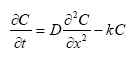
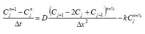
where C is concentration, D is diffusion coefficient (in this case D/R, R = retention coefficient), k is decay coefficient (also in this case k/R), x and t are distance (depth) and time. Discretising this equation:
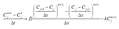
Rearranging:
Including a weighting factor:
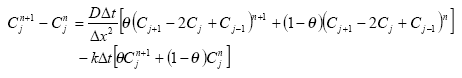
Collating time terms:
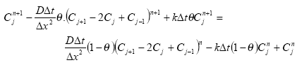
Then:
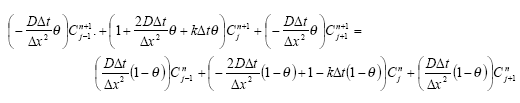
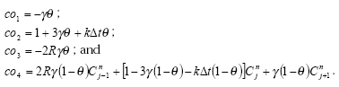
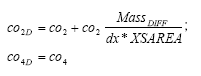
If D = D/R then ![]() and the equation is rewritten in the form
and the equation is rewritten in the form
![]()
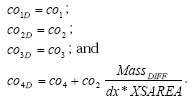
then the coefficients co1 to co4 are:
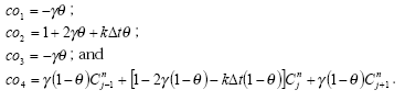
The simulation in the subsurface uses a weighting factor θ= 0.5 (Crank-Nicolson scheme).
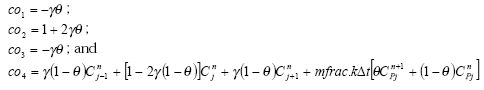
2. Discretisation of First Layer
The first layer, C1, is the water column concentration. This concentration is at the river bed, which is a distance of δx/2 from the centre of the second layer. Also, the water column concentration is not affected by the retention factor, R. This means that when calculating transport from layer 1 to layer 2 (j = 2) an adjustment is made such that:
The coefficients co1 to co4 for j = 2 then become (again with ![]() ):
):
3. Pesticide Decay to Metabolite
Decay occurs in the pesticide. A fraction of the decayed amount becomes metabolite. Decay of the metabolite itself is not considered at this stage. For the pesticide component, the terms above (with decay) are applied. For the metabolite component, the decayed pesticide is an additional source, independent of metabolite concentration. Linear decay is

which is discretised as
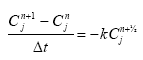
With inclusion of a weighting factor, this equation becomes:
![]()
The terms applied to the solution to pesticide diffusion are as shown in the previous section. The amount of decayed pesticide is given by:
Pesticide Decayed Amount
![]()
The amount is multiplied by a fraction (mfrac) and added to the metabolite concentration. Thus, the final terms applied in the solution of metabolite diffusion are:
4. Solution Technique in Subsurface
The above equations for pesticide diffusion in the subsurface are solved using an implicit scheme. The equations
![]()
are combined to give:
![]()
Rearranging the terms gives:
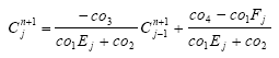
Shifting ![]() back by j gives
back by j gives ![]()
Therefore:
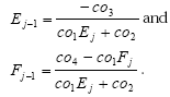
The first (EF) sweep is performed using a boundary condition at j = jmax where Cjmax-1 = Cjmax. In other words, E = 1, F = 0. The second sweep is performed with a boundary condition at j = 1, where C1 = Cbnd.
5. Solution Technique Between Subsurface and Water Column
Calculations during a MIKE 11 AD timestep are performed in the following sequence:
- The transport equation coefficients (co1, co2, co3, co4) in the water column are found.
- The first sweep of the pesticide diffusion equations is performed to find the E and F variables, using the previous water column concentration as the boundary condition. The first component to be solved is the pesticide, which can include decay. The decayed amount (a fraction of which can become a metabolite) is then stored. The first sweep of the metabolite component is then performed, which includes the decayed amount from the pesticide component.
- The E and F variables are then used to calculate the transport between the subsurface and the water column, which is incorporated into the transport equation coefficients (co1, co2, co3, co4) in the water column. Alternative 2 (Section 0), where the change in mass within the subsurface is calculated, is used to determine transport.
- The AD equation in the water column is then solved.
- The final sweep of the pesticide diffusion equations is then performed, using the updated water column concentration from step 4.
Thus, the subsurface calculations are made implicitly within the MIKE 11 AD solution scheme.
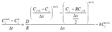
6. Transport Between Subsurface and Water Column
The transport of pesticide (and metabolite) between the subsurface and the water column is calculated to give additional components to the terms of the AD solution scheme in the water column. The transport of material from subsurface to the water column can be found in two ways. The first is given by:

where transport is considered to be transport between the first layer in the subsurface (C1), which has the same concentration as in the water column (CW), and the second layer in the subsurface (C2).
It appears that the high concentration gradients in the first layer mean that the calculation of transport is prone to truncation errors. This results in a calculation of transport from MIKE 11 AD to the subsurface that does not conserve mass. Nevertheless, the solution using a calculation of transport is described below. At the moment the second alternative, in which transport is calculated from the differences in total mass in the system over a timestep, is implemented in the model.
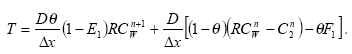
6.1 Alternative 1: Transport Calculation using Concentration Gradients
Discretisation of the transport equation gives the following. Note that there is no retention in the water layer, so when D = D/R, CW should be modified:
Including a weighting factor:
As discussed in the previous section, the EF sweep of the subsurface layers is performed prior to calculation of transport between subsurface and water column. The EF sweep provides the equation:
Combining gives:
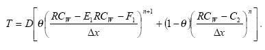
Expanding:
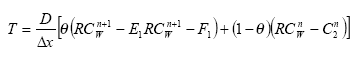
Collating time terms:
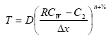
Transport T is mass rate per unit area. Therefore the mass entering the water column is T*Width*dx*δt, where Width is width of MIKE 11 cross-section, dx is distance between successive grid points and t is the timestep.
The AD equation in MIKE 11 solves concentration in the water column. Therefore in order to include this transport into MIKE 11 an expression of concentration is required. The volume of water that the transported mass is entering is given by XSAREA*dx, where XSAREA is the cross-sectional area of the grid point.
Further, the transport between the water column and layer 2 acts over a distance of half a depth interval (δx/2).
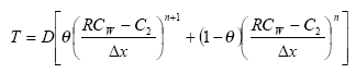
Finally, the terms of the MIKE 11 AD equation (for the water column) are modified so that:
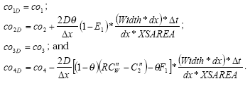
6.2 Alternative 2: Transport Calculation using Total Mass
The boundary conditions are set so that there is no transport of pesticide through the bottom layer of the subsurface (at j = jmax). This means that any change in mass in the subsurface is a result of transport through the top layer (from j = 1 to j = 2), or through decay. The transport between subsurface and water column therefore requires calculation of the difference in mass between successive timesteps.
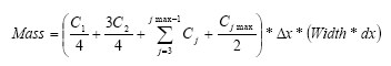
As discussed in Section 5, transport between subsurface and MIKE 11 is done at the end of the EF sweep in the water column and in the subsurface (step 3). This means that a preliminary calculation of the concentrations in the subsurface has to be performed. At this point in a timestep the mass in the subsurface is calculated using Simpson's Rule. Note that the first layer is actually the water concentration and is not included in the mass calculation. However, the concentration at the water / subsurface boundary is equal to C1 and is included in the calculations. The mass calculation is performed at time n+1:
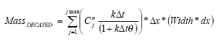
For pesticide (which decays), the amount entering the subsurface is equal to the amount decayed plus the change in mass:
![]()
For metabolite, the amount leaving the subsurface is equal to the total decayed amount of pesticide in the subsurface less the change in metabolite mass:
![]()
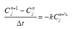
The discretised equation for linear decay is:
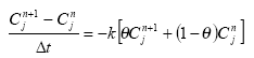
where C is concentration, k is decay coefficient, t is timestep.
The amount decayed is ![]() .
.
Combining, the decayed concentration over a timestep is given by:
![]()
Thus, the mass of decayed pesticide is given by:
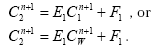
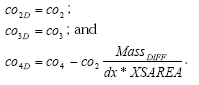
The mass is then included in the terms of the MIKE 11 AD equation (for the water column). This is done by comparing the equations:
![]()
Somehow these two equations can be combined. I think it may have something to do with
![]() , but
, but ![]() has already been
has already been
incorporated into co4.
In any case, the final terms for pesticide are:
![]()
I'm not sure about this, but it seems to work. Another alternative is
which should be the same thing?
The final terms for metabolite are:
7. Sedimentation in Water Column
The exchange (transport) of pesticide between the pore water of the first sediment layer and the water column is described by the differential equation:
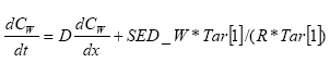
CW denotes the dissolved concentration (g/m3) of pesticide in the water column and the pore water, equal to Cd in the NERI report.
D denotes the diffusion coefficient (m2*h-1)
R denotes the retention factor (dimensionless)
Sed_W denotes the sedimentation of sorbed pesticide (g-pesticide*m-2*h-1). Sed_W is calculated by the existing MIKE 11 model as the product of the settling velocity of the particles, VS (m/hour), and the concentration of sorbed pesticide, CS, (g-pesticide*m-3) in the water column. Hence, Sed_W = VS*CS
Tar[1] denotes the area of the sediment surface (m2) and is given by the existing MIKE 11 model.
For the metabolite the same equation should be used.
8. Inclusion of Sedimentation into Surface Boundary Condition
The equation above is an additional source or sink to the AD solution scheme in the water column. The equation can be simplified to give:
Transport = ![]()
where transport in this case is that from subsurface into / out of the water column. With this additional term, considering that SED_W is VSCS and that surface area cancels out, gives the following:
![]()
CS is calculated explicitly at the end of a timestep. As such, this additional term is included at time increment (n):
![]()
This additional component of transport is added to the existing transport components (concentration gradient and decay) as mass, so that:
![]()
This is then included into the terms of the MIKE 11 AD equation as discussed in Section 0.
9. Stability and Discretisation of Linear Decay
The equation for linear decay is:
![]()
where C is concentration, k is decay coefficient, δt is timestep. This can be discretised as
Using a weighting factor:
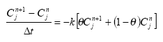
Expanding:
![]()
A condition of this equation is that the concentration after decay cannot be less than zero. Therefore:
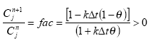
This is a limiting condition for linear decay, which could conceivably be reached in a model simulation depending on selection of decay rate and timestep. To ensure that the concentration after decay is greater than zero, the weighting factor is modified locally. Therefore rearranging the above equation produces the following conditions:
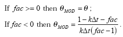
This means that the material is completely decayed in one timestep, and is applied such that stability is maintained in the solution.
10. Application in MIKE 11
The parameters to be used in the pesticide diffusion simulation are read from a pfs file called "PESTICIDE_DIFFUSION.TXT", which is located in the active directory. MIKE 11 will activate the pesticide diffusion component on the existence of this file.
Information in the pfs file includes details on the parameters associated with each pond type and each location. Also, the AD component numbers in the MIKE 11 AD setup allocated as pesticide and metabolite must be specified.
Output from the subsurface simulation is via a 'csv' format file, which is a comma or semi-colon delimited file that can be easily opened using Microsoft Excel. Results are presented at each timestep and at each pond location. An additional output file can be included that prints out a depth profile of concentrations at a given time.
The transport between subsurface and water column due to sorbed sediment is implemented only when the pesticide water quality module is activated. This module simulates the interactions. At present, this module simulates interactions between dissolved and sorbed pesticides both in the water column and subsurface. This will be modified so that this model replaces the subsurface interactions.
Note that all parameters applied in the model (diffusion, decay, etc) are input in units of grams (g), metres (m) and hours (h). Output from the subsurface simulation (csv text file) is in the same units.
11. Analytical Test
The test assumes that:
the concentration in the water column remains constant
there is no decay
In other words, the test is checking only diffusion through the sediment. The analytical solution is:
The following parameters are applied:
depth interval δx = 0.4 mm
D = 0.00013 m2/h
R = 400
Depmax = 0.05 m (this does not affect the results)
Time = 28 days
The MIKE 11 setup for this situation was a 20 m wide uniform channel with a depth of 100 m. A uniform initial concentration in the water column of CW = 1 g/m3 was applied. As the cross-section is very deep, the concentration does not change significantly from the initial value. The simulation was performed for 28 days at a timestep of 1 hour. The comparison to the analytical solution is shown below.
The comparison shows that the model compares well to the analytical solution, but does not fit exactly. Comparison between analytical and numerical solutions is shown as the percentage error of the total mass at the end of the simulation. As shown, the maximum errors occur at the start of the simulation (3.6% initially), and rapidly reduce – after 6 timesteps the incremental error is less than 0.1%.
12. Comparison to Excel Solution, No Decay
A test was run and compared to results from a solution developed in an Excel spreadsheet. Again, the concentration in the water column is assumed to be constant. While this is not verification to an analytical solution, it does eliminate potential errors in the numerical scheme and coding and ensures mass conservation.
The test assumes that:
depth interval δx = 0.001 m
D = 0.001 m2/h
R = 10
Depmax = 0.10 m
Timestep t = 300 s
Initial Concentration = 0
Water Concentration = 1
Decay = 0 /hr
Mfrac (fraction of pesticide decay that becomes metabolite) = 1.0
The receiving water was considered to be an enclosed volume of width 20 m, length 25 m and depth 1 m (Volume = 500 m3), which for a concentration of 1 g/m3 gives a mass in the water column of 500 g. The results for the first 10 timesteps are shown below.
The graph shows that the predicted mass in the subsurface is accurate, which indicates that the formulation of diffusion in the subsurface is working as expected. There is some error between the solutions in the water column. The extent of this error is investigated in the next test.
13. Comparison to Excel solution, with Decay
The same test as above was re-run using a pesticide decay rate in the subsurface of 23 /hr.
The maximum mass loss error of 0.1% occurs at the first timestep and diminishes as the simulation continues. While the previous test shows some discrepancies between model predictions and the Excel solution, this test shows that there is hardly any mass loss from the entire system.
Finally, the plot below shows the concentration profiles after 10 hours simulation for both the case without decay and the case with decay.
14. Example of PESTICIDE_DIFFUSION.txt
[PESTICIDE_DIFFUSION]
[Model_Parameters]
Pesticide_Component_No = 1
Metabolite_Component_No = 2
Output_File = 'pesticide_diffusion_outputn.csv'
Full_Output_ts = 100
EndSect // Parameters
[Pond_Parameters_List]
[Pond_Parameters]
Diffusion = .0015
Retention = 400
Metabolite_Fraction = 1.0
Decay = 0.001
dx = 0.0002
Depmax = 0.1
EndSect // Parameters
[Pond_Parameters]
Diffusion = .0015
Retention = 800
Metabolite_Fraction = 1.0
Decay = 0.002
dx = 0.0002
Depmax = 0.1
EndSect // Parameters
EndSect
[Pond_Locations_List]
[Pond_Locations]
Pond_Branch = 'TEST_VERIF_copy'
Pond_Grid = 150
Pond_Type = 1
EndSect
[Pond_Locations]
Pond_Branch = 'TEST_VERIF'
Pond_Grid = 100
Pond_Type = 2
EndSect
EndSect
EndSect // PESTICIDE_DIFFUSION
Version 1.0 Maj 2004, © Danish Environmental Protection Agency