| Bottom | | Front page |

Environmental Project no. 951, 2004

Comparisons of Energy Consumption for Refrigeration in Supermarkets

Contents

Preface

Resume

Summary

Nomenclature

1 Introduction

2 Layout of refrigeration systems

• 2.1 Conventional refrigeration systems
• 2.2 Cascade refrigeration systems
• Figure 2.1. Layout of the isoi-2 and iso-4 systems
• 2.3 Layout of refrigeration section in shop
• Figure 2.3. Layout principle for refrigeration appliances in Shop
• 2.4 System sizes

3 Measuring program

4 Data handling

• 4.1 Data used
• 4.2 Calculation of refrigeration output and power Consumption
• 4.3 Calculation of comparable energy consumptions

5 Comparisons

• 5.1 Measured and calculated power/energy consumption
• 5.2 Mean coefficient of performance and carnot efficiency
• 5.3 Consumption based on mean coefficient of performance
• 5.4 Consumption based on reference shop and actual cop
  • 5.4.1 Specified appliance data/store data
  • 5.4.2 Specified load profile

6 Conclusion

7 Further analysis

8 Project organisation

Appendix A

Appendix B

Appendix C

Appendix D

Appendix E

Appendix F

Preface

The project described in this report was aimed at devising methods for comparing in a correct way the energy consumption of various refrigeration system lay-out in supermarkets of approximately the same size. Measurements have been performed in four supermarkets.

The project was carried out in collaboration with Danfoss A/S, Findan A/S, ISO A/S, Institute for Product Development, and York Refrigeration A/S. Funding was received from the Danish EPA Program for Cleaner Products.

The conclusion in this report are entirely my responsibility.

Lyngby, 18 March 2004

Hans Jørgen Høgaard Knudsen,
Project leader

Resume

Formålet med det her omtalte projekt har været at sammenligne energiforbruget til køling i fire supermarkeder af sammenlignelig størrelse men med forskellig opbygning af køleanlægget. To af supermarkederne har nyudviklede kaskadeanlæg med CO₂ i lavtemperaturkredsen og R404A i højtemperaturkredsen og de to andre supermarkeder har konventionelt opbyggede køleanlæg med R404A. Energiforbruget er blevet målt over en periode på 5 måneder (1/8 til 31/12 2003). Da de fire anlæg dels har forskellig størrelse dels arbejder med forskellig kondenseringstemperatur på grund af varmegenvinding kan det målte energiforbrug ikke sammenlignes direkte. Der beregnes derfor et energiforbrug for et fiktivt supermarked baseret på de målte forbrug korriget til en specificeret kondenseringstemperatur.

Der er anvendt to modeller til beregning af et sammenligneligt energiforbrug. Den første model er baseret på en skalering af energiforbruget idet der som skaleringsfaktor er benyttet forholdet mellem det nominelle energiforbrug for den valgte reference butik og det nominelle energiforbrug for den aktuelle butik. Det nominelle behov er beregnet på grundlag af butikkens specifikation af forbrug i køle- og frostgondoler, kølereoler samt køle- og frostrum. Den anden model er baseret på en påtrykt belastning på henholdsvis køl og frost. Den påtrykte belastning er baseret på målingerne for måleperioden. På grundlag af disse målinger er opstillet relative belastningsprofiler. Det relative belastningsprofil udtrykker det øjeblikkelige kuldebehov som procent af det maksimale kuldebehov i hele måleperioden. For referenceanlægget er benyttet en maksimal belastning på kølesiden på 110 kW og en maksimal belastning på frostsiden på 40 kW. Endvidere er anlæggenes middel COP (forholdet mellem leveret kuldeydelse og forbrugt energi) i måleperioden beregnet.

Baseret på en skalering er energiforbruget for kaskadeanlæggene inklusiv energiforbrug til cirkulationspumpe ca. 2/3 af energiforbruget for de konventionelle anlæg. Men denne metode må imidlertid forkastes da den beregnede køleydelse for referenceanlægget afhænger af hvilket anlæg der er anvendt til beregning af køleydelsen. Årsagen hertil er metodens store følsomhed over for de nominelle data.

Energiforbruget beregnet på grundlag af et reference belastningsprofil er, inden for måleusikkerheden, ens for de to kaskadeanlæg og det ene af de konventionelle anlæg. De sidste konventionelle anlæg har et væsentligt større energiforbrug, hvilket må tilskrives den valgte kompressorbestykning.

Samme resultat fås ved af anvende belastningsprofilet sammen med middel COP for måleperioden.

For kaskadeanlæggene er energiforbruget til cirkulationspumpen ca. 10% af det totale energiforbrug. Det vil være muligt at reducere energiforbruget til cirkulationspumpen da den kører ureguleret dvs. med maksimalt flow uanset det øjeblikkelige behov.

Den endelige konklusion er, at kaskadeanlæggene har samme energiforbrug som et veldimensioneret konventionelt anlæg og det vil være muligt at reducere energiforbruget ved regulering af cirkulationspumpen.

Summary

The aim of the project presented in this report has been to compare the energy consumption for refrigeration in four supermarkets of approximately the same size but with different layout of the refrigeration system. Two of the supermarkets have newly developed cascade refrigeration systems with CO₂ in the low-temperature circuit and R404A in the high-temperature circuit. All the display cases were cooled by CO₂ with dry-expansion evaporators in the freezers and flooded evaporators in the refrigerators. The other two supermarkets have conventional multiplex refrigeration systems with R404A as refrigerant and dry-expansion evaporators in all display cases. The energy consumption was measured during a period of five month (1/8 – 31/12 2003). The energy consumption of the four systems cannot be compared directly because the systems were not the same size and their condensation temperatures were different due to heat recovery. Therefore, a reference supermarket is used, where the energy consumption is based on the measured energy consumptions corrected to the same reference condensations temperature.

Two models have been used to estimate the corrected energy consumption. The first model is based on a simple scaling factor calculated as the ratio between the nominal cooling capacity of the reference supermarket and the nominal cooling capacity of the actual supermarket. The nominal cooling capacity is calculated from the specification of the cooling needs for the individual display cases. The second model uses a prescribed load profile for the low and high temperature circuits of the refrigeration system. The load profile used is based on the measured load profile of one of the supermarkets during the period of measurement. The measured load profile is expressed as the ratio between the measured load and the highest load in the period of measurement. For the reference system the maximum high temperature load is set at 110 kW and the maximum low temperature load is set at 40 kW.

The mean COP (the ratio between the cooling load and the power supplied) has been calculated for the whole period of measurement.

According to the first model (scaling factor), the energy consumption of the cascade plants, including the pumping power for the flooded evaporators, is 2/3 of the energy consumption of the conventional multiplex system. This model has later been rejected because the calculated cooling load for the reference supermarket depends on which supermarket is used as a basis for the calculation, whereas only the power consumption of the reference supermarket should depend on which supermarket is used as a basis. The differences in cooling loads seem to be caused by a very high dependency of the nominal data.

According to the second model (load profile), the calculated energy consumptions of the two cascade systems and one of the multiplex systems were the same within the degree of measuring accuracy. The last multiplex system has a much higher energy consumption and the reason for this must be a lower efficiency of the compressors used.

For the cascade systems the energy consumption of the circulation pump for the flooded evaporators is approximately 10% of the total energy consumption. It is possible to reduce the energy consumption of the circulation pump by adjusting the capacity of the pump to the needs. At present the pump is running at full capacity independently of the actual need.

The over-all conclusion from the comparisons is that the new cascade systems have an energy consumption equal the energy consumption of a well dimensioned conventional refrigeration system and that it is possible to lower the energy consumption of the cascade system by implementing a control strategy for the circulation pump.

Nomenclature

1 Introduction

In connection with the phasing out of CFC and HCFC refrigerants it is being discussed whether the refrigerant in new systems should be HFC or natural substances. The problem with HFC refrigerants is their very high greenhouse effect (GWP), which in future may lead to a phasing out of this group of refrigerants also. In Denmark their use is prohibited in small and large systems from January 1^st 2007. Natural refrigerants do not have this drawback but are often either flammable (HC refrigerants) or toxic (ammonia). An alternative, which is neither flammable nor classified as toxic, is carbon-dioxide (CO₂). CO₂ does, however, have some drawbacks. Firstly, the critical temperature is very low (31°C). This has a negative effect on efficiency at one stage operation when ambient temperatures are close to or above the critical temperature. Secondly, the triple point pressure is greater than the atmospheric pressure (5.18 bar). This puts special demands on installations of safety valves, since any blow-off of liquid will result in solid CO₂ being formed. A system that does not suffer from the first disadvantage is a cascade system with CO₂ in the low-temperature circuit and, e.g., propane or propylene in the high-temperature circuit. The high-temperature circuit can be very compact with a small amount of refrigerant, which can minimise the danger of fire.

The present investigation has compared the energy consumptions of two conventional systems with R404A with two newly developed cascade systems with CO₂ in the low-temperature circuit and R404A in the high-temperature circuit. Because of the location it has not been possible to get permission to use propane/propylene in the high-temperature circuit. Therefore, R404A has been used. The amount of R404A used is, however, very small compared to that used in conventional systems.

2 Layout of refrigeration systems

• 2.1 Conventional refrigeration systems
• 2.2 Cascade refrigeration systems
• Figure 2.1. Layout of the isoi-2 and iso-4 systems
• 2.3 Layout of refrigeration section in shop
• Figure 2.3. Layout principle for refrigeration appliances in Shop
• 2.4 System sizes

2.1 Conventional refrigeration systems

The ISO-2 and ISO-4 systems are conventional systems of the parallel type with separate circuits for cooling and freezing and one-stage compression. The refrigerant used is R404A. Direct dry-expansion evaporation takes place in the cooling and freezing appliances and condensation takes place in air-cooled condensers mounted on the roof of the building. ISO-4 has a heat exchanger between the cooling and freezing circuits, but it was used during the period of measurement. Furthermore, in this system heat exchangers are mounted for heat recovery from super-heating and condensation. Figure 2.1 shows the construction, in principle.

2.2 Cascade refrigeration systems

The ISO-1 and ISO-3 systems are the newly developed cascade systems. CO₂ is used in both cooling and freezing appliances. Dry expansion is used in freezing appliances. CO₂ compressors compress the evaporated CO₂ to the pressure in the cooling circuit. Flooded evaporators with pump circulation are used in the cooling appliances. In the cascade cooler evaporating R404A is used to condense the CO₂ vapour. Compressors compress the R404A to the condensation pressure and the R404A vapour condensates in a water-cooled condenser. The cooling water gives off the condensation heat to the surrounding air in dry-coolers placed on the roof. ISO-1 has a heat recovering heat exchanger, which delivers all heating to the shop. Figure 2.2 shows the principle layout of the cascade system.

Figure 2.1. Layout of the ISOI-2 and ISO-4 systems

Figure 2.2. Layout of the ISOI-1 and ISO-3 systems.

2.3 Layout of refrigeration section in shop

All of the four plants are similar, in principle, as to the location of the refrigeration appliances in the shop. Figure 2.3 below illustrates the layout principle.

Figure 2.3. Layout principle for refrigeration appliances in shop.

2.4 System sizes

The sizes of the four systems are shown in table 2.1 below.

Table 2.1. System sizes

Table 2.1 shows that the four systems are different in size, both in absolute terms and in terms of relative size of the different elements.

All systems have pulse-width modulated control valves on all evaporators.

3 Measuring program

Power consumption, compressor and condenser capacity used, suction and discharge pressures of the compressors, the openings of the injection valves, superheat temperature at evaporator outlet, and air temperature of all evaporators were measured on all four systems. The in- and outdoor temperatures and the relative humidity in the shops were also measured.

4 Data handling

• 4.1 Data used
• 4.2 Calculation of refrigeration output and power Consumption
• 4.3 Calculation of comparable energy consumptions

4.1 Data used

Most of the measurements were taken every two minutes. Due to the large amounts of data, hourly means were used in the calculations.

Appendix F contains examples of the computed data from all four systems.

4.2 Calculation of refrigeration output and power consumption

The specifications from the manufacturers were used to set up a formula for calculating the volumetric and isentropic efficiency of the compressors as a function of the pressure across the compressor and the condensation temperature.

The formulas reproduce the data of the manufacturers in most of the temperature range better than 1% regarding refrigeration capacity and better than 2% regarding power consumption.

Appendix A gives the information on the compressors in more detail.

With the measured pressures and temperatures and the compressor capacity used, the formulas above yield refrigeration capacity and power consumption (See Appendix E). The power consumption calculated on the basis of compressor data was compared to the power consumption measured in order to get an estimate of the accuracy of the model.

The actual coefficient of performance (COP) and the Carnot efficiency were also calculated. Since the condensation pressure can be influenced by heat recovery, a corrected COP corresponding to a condensation temperature of 30C was also calculated using the compressor models shown above.

4.3 Calculation of comparable energy consumptions

Since the four refrigeration systems were different in size, their energy consumptions could not be compared directly. Therefore, the energy consumption of a fictive supermarket with a reference load but with the COPs measured was calculated. The resulting energy consumptions were directly comparable, since the measured pump energy was added to the calculated energy consumption of the compressors of ISO-1 and ISO-3.

The energy consumption was calculated for each day and for the period of measurement as a whole by summing the energy consumptions per hour. The energy consumptions per hour were calculated on the basis of hourly means of the power consumption.

Two models were used to calculate comparable energy consumptions. The first model was based on a reference shop with a given specification of cooling and freezing gondolas, cooling racks, and cold and freeze storage. Appendix D gives a further description. The other model is based on the given cooling load and freezing load. This load is based on measurements made during the period 1/8 – 31/12, 2003. On the basis of these measurements relative load profiles were calculated for each of the four systems. The relative load profile expresses the immediate refrigeration requirement as a percentage of the maximum refrigeration requirement during the whole period of measurement. The relative load profiles for the four systems were almost identical. This can be seen in figure 4.1, which shows the relative cooling load for the period 1/9 - 7/9, 2003. Appendix C shows the relative load profiles of the entire period of measurement and for cooling and freezing in the period 1/9 - 7/9, 2004. The relative load profile of the ISO-2 system was used in the further calculations. For the reference system a maximum load of 110 kW was used on the cooling side and a maximum load of 40 kW was used on the freezing side. Appendix E gives a further description of the method.

Figure 4.1. Relative load profile for cooling section

5 Comparisons

• 5.1 Measured and calculated power/energy consumption
• 5.2 Mean coefficient of performance and carnot efficiency
• 5.3 Consumption based on mean coefficient of performance
• 5.4 Consumption based on reference shop and actual cop
  • 5.4.1 Specified appliance data/store data
  • 5.4.2 Specified load profile

5.1 Measured and calculated power/energy consumption

The measured energy consumption of ISO-2 and ISO-4 cannot be compared directly with the calculated energy consumption, since the measured energy consumption includes the consumption by anti sweat heaters, fans and defrosting. A correction was made for these loads. The number of defrosting events and their duration were estimated on the basis of the measurements. The calculated energy consumption was based on the assumption that the defrosting heaters were in use during the entire defrosting event. One of the power meters for ISO-4 was not working. But in February 2004 both of the power meters were functioning. Thus power consumption measured in February can be compared with the calculated consumption. The deviation between the corrected energy consumption per day and the calculated consumption per day in February is less than 11% for ISO-2, while ISO-4 produces a deviation of about 40% when corrections are made for anti sweat heat eT_c. Without corrections the deviation is less than 10%. For ISO-1 and ISO-3 the measured and calculated consumptions are directly comparable if the circulation pump power consumption is added to the calculated consumption. For ISO-1 the deviation between measured and calculated consumption is 20%. The power measurement on ISO-3 has a calibration error since the measured power consumption is much greater than the installed compressor power consumption. In February 2004 an attempt was made at applying a correct calibration factor, but the measured power consumption was now much lower than the calculated consumption. This power meter should, therefore, be re-calibrated.

(NB! In the following, measured consumption is the consumption calculated on the basis of measured used compressor capacity and the operational parameters for the compressors).

5.2 Mean coefficient of performance and Carnot efficiency

The mean coefficient of performance and the Carnot efficiency was calculated for the period 1/8 - 31/12 2003 on the basis of condensation and evaporation temperatures, irrespective of the circulation pump consumption. The result is shown in table 5.1 below.

Table 5.1. Mean COPs and Carnot efficiencies

In the table above, index C stands for the cooling circuit and index F stands for the freezing circuit. Index cor indicates that the mean has been calculated for a fixed condensation temperature of 30°C. For the cascade systems the index tot indicates that the data for the freezing circuits of the cascade system have been converted into a total COP/Carnot efficiency for the freezing circuit. This has been done adding the part of the consumption in the high-temperature circuit, which goes to the freezing circuit to the consumption of the freezing circuit. This corresponds to having a cascade system for freezing alone.

Table 5.1 shows that the cascade systems have a higher COP than the other two systems. It also shows that the systems have almost the same Carnot efficiency in the cooling circuit, whereas ISO-4 has a considerably lower Carnot efficiency in the freezing circuit.

5.3 Consumption based on mean coefficient of performance

Based on the above means, energy consumption for the period of measurement was calculated for the fictive system with the reference profile as load. The result is shown in table 5.2 below.

In table 5.2, (corrected) indicates that the energy consumption was calculated on the basis of means for COP_Cor with a fixed condensation temperature of 30°C, while (measured) indicates that the energy consumption was calculated on the basis of means for COP with the measured condensation temperature.

Table 5.2. Energy consumption based on mean COP for the period 1/8-31/12 2003

As can be seen in table 5.2, ISO-1, ISO-2, and ISO-3 have almost the same corrected consumption, whereas ISO-4 has consumption, which is almost 20% greater. With the measured mean for COP, ISO-3 has the lowest consumption, the consumption of ISO-1 is about 10% higher, that of ISO-2 is about 30% higher, and that of ISO-4 is about 50% higher than for ISO-3. This shows that the condensation temperature has a major influence on energy consumption. ISO-1 has operated with a mean condensation temperature of 28 °C, ISO-2 with a mean of 38 °C, ISO-3 with a mean of 28 °C, and ISO-4 with a mean of 32 °C during the first half of the period of measurement and 38 C during the second half. This change in condensation temperature is due to the heat requirement, which is met through heat recovery from the condensers. Figure 5.1 shows the condensation temperatures during the period of measurement.

Figure 5.1. Condensation and evaporation temperatures

Even though ISO-1 and ISO-3 are indirectly air-cooled via a cooling water circuit, they have lower condensation temperatures than the systems ISO-2 and ISO-4 which have directly air-cooled condensers. Since the cascade systems have the same refrigerant in the high-temperature circuit as the classic systems, it must be concluded that the cascade systems have more efficient/larger heat transfer surfaces.

Figure 5.1 shows that the cascade systems operate with an evaporation temperature of –8 °C in the cooling circuit whereas the other two systems operate with a temperature of –15 °C. In the freezing circuits the evaporation temperature is –30°C in the cascade systems and –35 °C in the other systems. Since the evaporators are similar in the four systems, the higher temperatures in the cascade systems can only be due to the heat conductivity of the refrigerant. Part of the higher evaporation temperature in the ISO-1 and ISO-3 cooling circuits can also be due to the fact that these have flooded evaporators in the cooling circuits. The higher evaporation temperature results in a better COP, which is, however, outweighed by the energy consumption of the circulation pumps. Table 5.2 shows that the energy consumption of the pumps is about 10% of the total consumption. But the pumps operate unregulated and thus with full capacity even when the load is low. Introducing a capacity regulation of the pumps can probably lower the energy consumption.

5.4 Consumption based on reference shop and actual COP

In the previous section the four systems were evaluated on the basis of means. Due to the varying operational conditions, this can give an erroneous picture of the true energy consumption. Therefore, a calculation was made for the reference system using the measured COP. Two methods were used to determine the load on the reference system. With the first method the measured consumption was scaled using a scaling factor based on the specified appliance/store data. With the second method the load is determined on the basis of a maximum load and a reference load profile.

5.4.1 Specified appliance data/store data

From hourly means of measured values of evaporation and condensation pressures, suction temperatures of the compressors, and applied compressor capacity the energy consumption was calculated on the basis of data from the manufacturers of the compressors. The consumption was corrected to consumption at a condensation temperature of 30°C, in order to eliminate the effects of different operation strategies on the condenser side (e.g., heat recovery).

Data on the refrigeration needs of each appliance and cooling/freezing store in the supermarkets weresupplied from the manufacture. These data were converted into nominal consumptions per appliance m and per store m ³. The consumption by the gondolas is given per circumference m in order to include the end gondolas. By this is taking into account that most of the gondolas are double gondolas.

Since the nominal consumption per appliance m and per store m ³ in the supermarkets is not equal (the appliances in the newest supermarkets have a lower nominal consumption), means for the four supermarkets were calculated. A reference supermarket was defined with 50m cooling and freezing gondolas, 35m cooling racks, 12m counters, 350m ³ cold storage, and 100m ³ freeze storage. These figures constitute means from the four supermarkets.

The energy consumption of each supermarket was converted to a consumption of the reference supermarket. This was done on the assumption that the ratio of nominal consumption to actual consumption is the same for the actual supermarkets and the reference supermarket. This means that the evaporation temperature of the reference supermarket is the same as the measured evaporation temperature.

The reference loads on the cooling and frost sections of the cascade systems were determined first. The load on the high-temperature section is the sum of the load from freezing appliances plus the power consumption of the low-temperature compressors and the load from the cooling appliances.

This method is described in more detail in Appendix D.

Figure 5.2 shows a comparison of the energy consumptions during September, which are similar to those of the rest of the period of measurement.

Figure 5.2. Energy consumption of reference shop based on measured energy consumptions (month)

Figure 5.3 shows a comparison of the energy consumptions during a single day (1 September 2003)

Figure 5.3. Energy consumption of reference shop based on measured energy consumptions (day).

Figures 5.2 and 5.3 show that the energy consumptions of the reference shop with data from ISO-1 and ISO-3 are about 2/3 of the energy consumptions of the reference shop with data from ISO-2 and ISO-4. But a critical viewing of the calculated energy consumptions of the reference shop shows that the loads on the reference shop are not the same with data from the four supermarkets. This is shown in figure 5.4 (load on cooling).

The loads on cooling for ISO-1 and ISO-3 are about 2/3 of the loads for ISO-2 and ISO-4. With respect to load on freezing, ISO-3 is different from ISO-1, ISO-2, and ISO-4. The load is considerably higher for these than for ISO-3, as shown in figure 5.5. This is in part due to difference in relative load q_measured/q_nominalt as shown in figures 5.6 and 5.7. These figures show that ISO-4 especially has a load profile, which is very different from those of the other three. This difference must be caused by a scaling factor, the nominal load, which is too uncertain.

The conclusion must be that, due to uncertain nominal refrigeration requirements, a "simple" scaling based on nominal refrigeration requirements does not give a true picture of the energy consumption of the supermarkets.

Figure 5.4. Cooling load for reference shop based on measured loads (day).

Figure 5.5. Freezing load for reference shop based on measured loads (day)

Figure 5.6. Relative load on cooling (day).

Figure 5.7. Relative load on freezing (day)

5.4.2 Specified load profile

As mentioned in section 4.3, relative load profiles were generated on the basis of measurements from the period 1/8 – 31/12 2003. The relative load profile expresses the immediate refrigeration requirement as a percentage of the maximum refrigeration requirement during the whole period of measurement. The relative load profiles for the ISO-2 system were used in the calculations. A maximum load on the cooling side of 110 kW and a maximum load on the freezing side of 40 kW has been used for the reference system.

This method is described in more detail in Appendix E.

The method corresponds to the method described in section 5.3, except that the actual COP was used here instead of the mean COP together with the load profile to determine the energy consumption.

Figures 5.8 and 5.9 show the reference load and the corresponding total power consumption based on hourly means (consumption by pumps included) for the reference system during a week where the load was high. Similarly, figures 5.10 and 5.11 show load and power consumption during a week where the load was low. Figures 5.9 and 5.11 show that ISO-1, ISO-2, and ISO-3 have the same power consumptions when the load is the same, whereas ISO-4 has considerably higher power consumption. The considerably higher power consumption of ISO-4 must be due to the lower Carnot efficiency of the compressors.

All shops have comparable ambient operation conditions: In- and outdoors temperatures and humidity in the shop (See figures 5.12 and 5.13).

Figure 5.8. Reference load with high load

Figure 5.9. Power consumption with high load

Figure 5.10. Load profile with low load

Figure 5.11. Power consumption with low load

Figure 5.12. Humidity and temperature conditions with high load

Figure 5.13. Humidity and temperature conditions with low load

6 Conclusion

Based on the above results it can be concluded that the cascade systems have the same energy consumption as a well-dimensioned conventional system.

Lower energy consumption in the cascade systems can be expected if the control of the circulation pumps is improved.

The energy consumption of the cascade systems can be further reduced by improving the algorithms controlling the electric power in connection with the defrosting of the flooded evaporators in the cooling section. During the period of measurement, the defrosting functioned in the same way as for dry evaporators. But when defrosting started, the flooded evaporators had a greater liquid content than the dry evaporators. Therefore, energy consumption can be reduced in two ways, firstly the direct electrical consumption by the defrosting heat elements can be reduced and secondly the indirect consumption by the compressors. The increased power consumption by the compressors is due to the fact that the liquid in the evaporators is evaporated by the heating elements and not as a result of advantageous cooling in the evaporator.

7 Further analysis

The data gathered will be analysed further to investigate whether the higher evaporation temperatures have a positive effect on the frosting over of the evaporators.

8 Project organisation.

The project has been carried out in collaboration with Danfoss A/S, Findan A/S, ISO A/S, Institute for Product Development, and York Refrigeration A/S with funding from the Danish EPA Program for Cleaner Products.

We are grateful to the firms for their contributions.

The following deserve special thanks:
Christian Bendtsen, Danfoss A/S
Alexander Cohr Pachai, York Refrigeration A/S
Mortens Juel Skovrup, IPU

Appendix A

ISO-1 Cascade system

Compressors

Efficiencies

Bitzer 6H-25.2Y with R404A

Volumetric efficiency

Etav=(avA+bvA*Tc)+(avB+bvB*Tc)*Phi
with Tc: Condensation temperature in °C and Phi as the pressure ratio P_c/P₀

The constants have been determined as shown below:

Isentropic efficiency

EtaIs = (aisA+bisA*Tc)+(aisB+bisB*Tc)*Phi+ (aisC+bisC*Tc) *Phi²
with Tc: Condensation temperature in C and Phi as the pressure ratio P_c/P₀

The constants have been determined as shown below:

With the determined constants, Bitzer's data are reproduced better than 1.2% for the refrigeration capacity and better than 3.7 % for the power consumption of the compressor for -40°C<T0<-5°C and 30°C<Tc<50°C.

Within the actual temperature range, the data for the refrigeration capacity are reproduced better than 0.2% and the data for the power consumption of the compressor are reproduced better than 2.3%.

Bitzer 2EC-4.2K with R744

Volumetric efficiency

EtaV=ac(Tc)*(Phi-1.235)+0.9247
with Tc: Condensation temperature in C and Phi as the pressure ratio P_c/P₀

The constants have been determined as shown below:

Ac=-0.111873903+0.0001737681367*Tc-
6.613978021E-5*Tc*Tc

Isentropic efficiency

EtaIs = A(T) + B(T)*Phi + C(T)*Phi*Phi

A = aA+bA*T+cA*T*T
aA = 0.7309844503      bA = 0.008370719891
cA = -0.0005993144145
B = aB+bB*T+cB*T*T
aB = -0.06575970538      bB = -0.002804107695
cB = 0.0005618800195
C = aC+bC*T+cC*T*T
aC = -0.001403356293      bC = -0.0004784304082
cC = -0.0001543907826

With the determined constants, Bitzer's data are reproduced better than 0.2% for the refrigeration capacity and better than 0.6 % for the power consumption of the compressor for -50°C<T0<-30°C and -20°C<Tc<-5°C.

Table A1. Comparison between data and fit for Bitzer 6H-25.2Y

Table A2. Comparison between data and fit for Bitzer 2EC-4.2K

Figure A1. Volumetric efficiency for Bitzer 6H-25.2Y

Figure A2. Isentropic efficiency for Bitzer 6H-25.2Y

Figure A3. Volumetric efficiency for Bitzer 2EC-4.2K

Figure A4. Isentropic efficiency for Bitzer 2EC-4.2K

ISO-2 Conventional system (Parallel system).

Compressors

Efficiencies

PresTcold 400/0062 with R404A

Volumetric efficiency

Etav=A+B*Phi
with Phi as the pressure ratio P_c/P₀
The constants have been determined as shown below:
A = 1.02740540205
B= - 0.03579218125

Isentropic efficiency

EtaIs=(aA+bA*Tc)+(aB+bB*Tc)*Phi+(aC+bC*Tc+
cC*Tc*Tc)*Phi*Phi
with Tc: Condensation temperature in C and Phi as the pressure ratio P_c/P₀

The constants have been determined as shown below:

With the determined constants, PresTcold's data are reproduced better than 2.5% for the refrigeration capacity and better than 5.6 % for the power consumption of the compressor for -50°C<T0<-20°C and 25°C<Tc<55°C.

Within the actual temperature range, the data for refrigeration capacity are reproduced better than 1.1% and the data for the power consumption of the compressor are reproduced better than 1.8%.

Table A3. Comparison between data and fit for PresTcold 400/0062

Figure A5. Volumetric efficiency for PresTcold 400/0062

Figure A6. Isentropic efficiency for PresTcold 400/0062

ISO-3 Cascade system

Compressors

Efficiency

Bitzer 4G-30.2Y with R404A

Volumetric efficiency

Etav=(avA+bvA*Tc)+(avB+bvB*Tc)*Phi
with Tc: Condensation temperature in C and Phi as
pressure ratio P_c/P₀

The constants have been determined as shown below:

Isentropic efficiency

EtaIs = (aisA+bisA*Tc)+(aisB+bisB*Tc)*Phi
+(aisC+bisC*Tc) *Phi²
with Tc: Condensation temperature in C and Phi as
pressure ratio P_c/P₀

The constants have been determined as shown below:

With the determined constants Bitzer's data are reproduced better than 1.2% for the refrigeration capacity and better than 4.2 % for the power consumption of the compressor for -40°C<T0<-5°C and 30°C<Tc<50°C.

Within the actual temperature range, the data for the refrigeration capacity are reproduced better than 0.4% and the data for the power consumption of the compressor are reproduced better than 0.6%.

Bitzer 2HC-3.2K with R744

Volumetric efficiency

EtaV = aC(Tc)*(Phi-1.232) +0.9280
with Tc: Condensation temperature in C and Phi as pressure ratio P_c/P₀
The constants have been determined as shown below:
aC = - 0.1119778613 + 0.0001747267099*Tc
- 6.59837705E-005*Tc*Tc

Isentropic efficiency

EtaIs = A(T) + B(T)*Phi + C(T)*Phi*Phi

A = aA+bA*T+cA*T*T
aA = 0.6460083817     bA = -0.001121194203
cA = -0.0008059707318
B = aB+bB*T+cB*T*T
aB = -0.009833249381     bB = 0.002792562938
bB = 0.0006477213502

C = aC+bC*T+cC*T*T
aC = -0.0100883472     bC = -0.001219987245
cC = -0.0001574917651

With the determined constants, Bitzer's data are reproduced better than 0.4% for the refrigeration capacity and better than 0.8 % for the power consumption of the compressor for -50°C<T0<-30/deg;C and -20/deg;C<Tc<-5°C.

Table A6. Comparison between data and fit for Bitzer 4G-30.2Y

Table A7. Comparison between data and fit for Bitzer 2HC-3.2K

Figure A7. Volumetric efficiency for Bitzer 4G-30.2Y

Figure A8. Isentropic efficiency for Bitzer 4G-30.2Y

Figure A9. Volumetric efficiency for Bitzer 2HC-3.2K

Figure A10. Isentropic efficiency for Bitzer 2HC-3.2K

ISO-4 Conventional system (Parallel system).

Compressors

High-temperature stage: 15 Copeland Scroll ZS75K4E-TDW
Refrigerant: R404A

Low-temperature stage: 7 Copeland Scroll ZF33K4E-TDW
Refrigerant: R744 (CO₂)

Efficiency

Copeland Scroll ZS75K4E-TDW with R404A

Volumetric efficiency

Etav = A0 + A1*Phi + A2*Phi² + A3*Phi³
with Tc: Condensation temperature in C and Phi as pressure ratio P_c/P₀
The constants have been determined as shown below:

Isentropic efficiency

Etais = A0 + A1*Phi + A2*Phi² + A3*Phi³ + A4*Phi⁴
with Tc: Condensation temperature in C and Phi as
pressure ratio P_c/P₀
The constants have been determined as shown below:

With the determined constants Copeland's data are reproduced better than 0.3% for the refrigeration capacity and better than 1.2 % for the power consumption of the compressor for -30°C<T0<7°C and 30°C<Tc<50°C.

Within the actual temperature range, the data for the refrigeration capacity are reproduced better than 0.2% and the data for the power consumption of the compressor are reproduced better than 2.3%.

The calculated volumetric efficiency is, however, greater than 1 which, according to Copeland, is due to the definition of geometric volume.

Copeland Scroll ZF33K4E with R404A

Volumetric efficiency

Etav = A0 + A1*Phi + A2*Phi²
with Tc: Condensation temperature in C and Phi as
pressure ratio P_c/P₀
The constants have been determined as shown below:

Isentropic efficiency

Etais = A0 + A1*Phi + A2*Phi² + A3Phi³
with Tc: Condensation temperature in C and Phi as
pressure ratio P_c/P₀
The constants have been determined as shown below:

With the determined constants Copeland's data are reproduced better than 2.5% for the refrigeration capacity and better than 3.2 % for the power consumption of the compressor for -40°C<T0<5°C and 30°C<Tc<50°C.

Within the actual temperature range, the data for the refrigeration capacity are reproduced better than 1.4% and the data for the power consumption of the compressor are reproduced better than 0.7%.

The calculated volumetric efficiency is, however, greater than 1 which, according to Copeland, is due to the definition of geometric volume.

Table A7. Copeland Scroll ZK75K4E

Table A8. Copeland Scroll ZF33K4E

Figure A11. Volumetric efficiency for Copeland Scroll ZS75K4-TDW

Figure A12. Isentropic efficiency for Copeland Scroll ZS75K4E-TDW

Figure A13. Volumetric efficiency for Copeland Scroll ZF33K4E-TDW

Figure A14. Isentropic efficiency for Copeland Scroll ZF33K4E-TDW

Appendix B

Means and maximum load

ISO-1

Number of data points: NTimeTot = 2646

T0F mean = -29.7 °C
TcF mean = -7.8 °C
T0C mean = -8.0 °C
TcC mean = 28.8 °C
qCmax = 171 kW 26 September at 11:00 hours
qFmax = 45 kW 9 December at 8:00 hours

ISO-2

Number of data points: NtimeTot = 3280

T0F mean = -34.7 °C
TcF mean = 36.4 °C
T0Cmean = -15.1 °C
qCmax = 176 kW 13 August at 16:00 hours
qFmax = 38 kW 3 October at 14:00 hours

ISO-3

Number of data points: NTimeTot = 3136

T0F mean = -29.9 °C
TcF mean = -7.8 °C
T0Cmean = -8.0 °C
TcC mean = 23.3 °C
qCmax = 145 kW 9 August at 16:00 hours
qFmax = 32 kW 14 October at 12:00 hours

ISO-4

Number of data points: NTimeTot = 2890

T0F mean = -35.6 °C
TcF mean = 34.5 °C
T0C mean = -14.4 °C
TcC mean = 34.1 °C
qCmax = 200 kW 31 August at 8:00 hours
qFmax = 56 kW 15 October at 11:00 hours

Appendix C

Comparisons of load profiles (Qactual/Qmax)

Figure C1. Load profile for cooling section for the period 1/8-31/12 2003

Figure C2. Load profile for freezing section for the period 1/8-31/12 2003

Figure C3. Load profile for cooling section for the period 1/9-7/9 2003

Figure C4. Load profile for freezing section for the period 1/9-7/9 2003

Appendix D

Reference shop. Load determined by scaling of appliance length/store size

Introduction

In order to compare the energy consumption of the different supermarkets, it was necessary to refer to a standard shop. The circumferences of the freezing and cooling gondolas, the lengths of the cooling racks and counters, and the volumes of the freezing and cold stores were set for the standard shop. In order to get the variation in the load included in the energy consumption, the ratio of the actual load to the nominal load was assumed to be constant. The nominal load was determined on the basis of the information from the manufacturer concerning the refrigeration requirements for the appliances and the stores.

Procedure for calculating comparable energy consumptions

The energy consumption was calculated on basis of the hourly means of measured evaporation and condensation pressures, compressor suction temperatures, and used compressor capacity, and the data from the compressor manufacturers. The power was corrected to power at a condensation temperature of 30°C to eliminate the influence from different operation strategies on the condenser side (e.g., heat re-circulation).

Data on the nominal refrigeration requirements of the individual refrigeration appliances and cooling/freezing storages is given for each supermarket. These data are converted to a nominal consumption value per appliance meter and per m ³ of store.

Since the nominal consumption per appliance meter and per m ³ of store was different for each supermarket (the nominal consumptions of the appliances in the newest supermarkets are lowest), a mean for the four supermarkets was calculated. A reference supermarket was defined with freezing and cooling gondolas with a 50m circumference, 35m cooling racks, 12m counters, 350m ³ cooling storage and 100m ³ freezing storage. This reference supermarket corresponds to a mean of the four supermarkets.

The energy consumption of each supermarket was converted to a consumption of the reference supermarket. This was done on the assumption that the relation between the nominal consumption and the actual consumption is the same for the actual supermarket and the reference supermarket. This means that the evaporation temperature of the reference supermarket is the same as the measured evaporation temperature.

The reference loads on the cooling and frost sections of the cascade systems were determined first. The load on the high-temperature section is the sum of the load from freezing plus the power consumption of the low-temperature compressors and the load from the cooling appliances.

Calculation of energy consumption based on data from the compressor manufacturers

"Measured" actual power consumption

Based on the measured data the refrigeration capacity and the power consumption at the reference condensation temperature can now be calculated as follows:

Actual volume flow is calculated on the basis of measured pressure ratio and suction temperature using the expression:

with:

: Actual volume flow through the compressor

: Volumetric efficiency

P_c Condensation pressure

P₀: Evaporation pressure

T_c: Condensation temperature

: Geometric stroke volume of the compressor

N_com: Number of compressors

I_ComCap: compressor capacity in use

The mass flow is, therefore:

with:

v(T₁,P₀): Specific volume at suction stop valve

T₁ Temperature at suction stop valve

P₀: Evaporation pressure

The "measured" refrigeration output is thus:

with:

h₁(T₁,v₁(T₁,P₀)): Enthalpy at suction stop valve

h₃(T₃): Enthalpy after condenser

T₃: Temperature after condenser

And the corrected "measured" power consumption is:

with:

h_2cor,is(T_2cor,is,v_2cor,is) Enthalpy after compressor at isentropic compression

: Isentropic efficiency

P_c.cor: Condensation pressure at reference condensation temperature

T_c,cor: Reference condensation temperature

Reference load

Conventional system

The refrigeration capacity for the reference supermarket with separate circuits for cooling and freezing are determined using the following procedure:

with:

and the power consumption is determined as:

with:

Cascade system

The refrigeration capacity and power consumption of the freezing section of the cascade system is calculated as indicated above when the system has separate circuits. The power consumption of the freezing section of the reference system is thus:

with:

The load from the cooling appliances and storage of the cascade system in the reference system is determined as:

with:

The total power consumption by the high-temperature section is determined as:

The total power consumption of the cascade system is, therefore:

Results

Figure D1 shows a comparison of the energy consumption per day for September 2003. The situation was quite similar during the rest of the measuring period.

Figure D2 shows a comparison of the power consumption (hourly means) for a 24-hour period (1 September 2003)

Figures D1 and D2 show that the energy consumptions of the reference shop with data from ISO-1 and ISO-3 are about 2/3 of the energy consumptions of the reference shop with data from ISO-2 and ISO-4. A critical examination of the calculated energy consumptions of the reference shop, however, shows that the loads are not the same for the reference shop with data from the four supermarkets, as shown in figures D3 (load on cooling) and D4 (load on freezing). ISO-1 and ISO-3 have loads on cooling which is about 2/3 of the loads for ISO-2 and ISO-4. The load on freezing for ISO-3 is considerably below the loads for ISO-1, ISO-2, and ISO-4. This difference in load is partly explained by difference in relative load, as shown in figures D5 and D6. These figures show that especially ISO-4 has a load profile which differs considerably from those of the other three. These figures show that ISO-4 especially has a load profile, which is very different from those of the other three. This difference must be caused by a scaling factor, the nominal load, which is too uncertain.

Conclusion

It must be concluded that a "simple" scaling based on nominal refrigeration requirement does not produce a true picture of the energy consumptions of the supermarkets because of uncertainty regarding the nominal refrigeration requirements.

Figure D1. Energy consumption per day in reference shop based on measured energy consumption (month)

Figure D2. Power consumption in reference shop based on measured energy consumption (day)

Figure D3. Cooling load in reference shop based on measured load (day)

Figure D4. Freezing load in reference shop based on measured load (day).

Figure D5. Relative load cooling (day)

Figure D6. Relative load freezing (day)

Appendix E

Reference shop

Energy consumption determined on the basis of reference load profile and actual COP

Introduction

In order to be able to compare the energy consumption of the different supermarkets, reference must be made to a standard shop. The load for freezing and cooling in the reference shop was determined on the basis of a load profile for the period 1/8 – 31/12 2003 and a maximum load for freezing and cooling respectively. A reference condensation temperature was set at 30°C.

Procedure for determination of reference load

On the basis of hourly means of measured refrigeration capacity for the period 1/8 – 31/12 2003 measurements from ISO-2 were chosen for the generation of a relative load profile. The relative load profile (q_rel) emerged as the relation between the momentary load (Q_actual) and the maximum load during the period (Q_max):

q_rel = Q_actual/Q_max

In Appendix B is shown the maximum load and the point when it was greatest. For the reference shop a maximum load of 110 kW on cooling and a maximum load of 40 kW on freezing were chosen.

ISO-2 was chosen as reference for the non-dimensional profile because the measurements on this system constitute the most complete set of measurements among the sets from the four systems. The load profiles from the four shops are compared in Appendix C.

Calculation of power consumption on the basis of reference load

Actual COP

Based on the measured data, the refrigeration capacity and the power consumption at the reference condensation temperature can be calculated as follows:

Actual volume flow is determined from the measured pressure ratio and suction temperature using the following expression:

with:

:	Actual volume flow through the compressor
:	Volumetric efficiency
Pc	Condensation pressure
P0:	Evaporation pressure
Tc:	Condensation temperature
:	Geometric compressor stroke volume
NCom:	Number of compressors
IComCap:	Compressor capacity in use

The mass flow is, therefore:

with:

The "measured" refrigeration output is then:

with:

and the corrected "measured" power consumption:

with:

h2cor,is(T2cor,is,v2cor,is):	Enthalpy after compressor at isentropic compression at reference condensation temperature
:	Isentropic efficiency
Pc.cor:	Condensation pressure at reference condensation temperature

T_c,cor: Reference condensation temperature

and thus:

Reference energy consumption.

Conventional system.

The reference loads for cooling and freezing are determined as:

and the energy consumption is determined as:

with:

Cascade system

The refrigeration capacity and power consumption of the freezing section of the cascade system is calculated as indicated above when the system has separate circuits. The power consumption of the freezing section of the reference system is thus:

with:

For the cooling section of the cascade system, the total load is the sum of the refrigeration load from the cooling appliances and cold store determined on the basis of reference load profile and condenser output for the freezing section determined as the sum of refrigeration output and power consumption:

with:

The total power consumption for the cascade system is, therefore:

Results

Figures E1 and E2 show hourly means of the reference loads and the corresponding total power consumption respectively for the four systems during the course of a week where the load was high. The power consumption of the pump is included for systems with pump circulation. Correspondingly, figures E3 and E4 show loads and power consumptions during the course of a week where the load was low. Figures E2 and E4 show that for the same load profile ISO-1, ISO-2, and ISO-3 had almost the same power consumptions, whereas the power consumption of ISO-4 was considerably higher.

All of the shops had comparable ambient operational conditions: in- and outdoor temperatures and humidity in the shops. See figures E5 and E6.

The reason for the considerably higher power consumption for ISO-4 must be attributed to the lower isentropic efficiency for the compressors, which were used under the existing operational conditions (pressure ratio). The actual pressure ratios were considerably higher than the ratios, which would correspond to the built-in volume ratio. The three other systems do not depend in the same way on the pressure ratio since their compressors are piston compressors. See Appendix A.

Conclusion

Based on the present results, it can be concluded that if the load profile is the same, then the cascade systems have the same power consumption as a conventionally constructed system of standard dimensions with piston compressors.

Figure E1. Reference load when load is high.

Figure E2. Power consumption when load is high

Figure E3. Load profile when load is low

Figure E4. Power consumption when load is low

Figure E5. Humidity and temperature conditions when load is high

Figure E6. Humidity and temperature conditions when load is low

Appendix F

Examples of result files

1 Introduction

Examples of results generated on the basis of the measured data are given below. Due to the fundamental differences in the construction of the systems, the result files are not entirely identical. But in pairs they are, i.e. e., ISO-1 and ISO-3 look alike, as do ISO-2 and ISO-4.

There are two types of files: The first one contains summed daily consumption/capacity for a month. The other one contains hourly values for a day.

The first part of the name of the file on monthly values is X_YYMM. The first part of the name of the file on daily values is X_YYMMDD where:

X: Specifies system (F: ISO-1, H: ISO, S: ISO-3 and V: ISO-4)
YY: Year (03 or 04)
MM: Month (January: 01, February: 02,.....,December:12)
DD: Day of the month (01,02,.....,31).

2 Monthly printouts. File type X_YYMMc.res

These files contain the calculated and measured energy consumption per day and differences between measured and calculated energy consumption.

ISO-1 and ISO-3:

ISO-2 and ISO-4:

3 Daily printouts. File type X_AAMMDDc.res

These files contain hourly means of evaporation and condensation temperatures, pressure ratios, volumetric and isentropic efficiencies, and power consumptions for freezing and cooling.

The printouts is the same for all four systems.

4 Daily printouts. File type X_AAMMDDfugt.res

These files contain evaporation and condensation temperatures, relative refrigeration outputs COP, Carnot efficiencies for cooling and freezing, inside and outside temperatures, and humidity in shop.

The files for the four systems are almost identical, but those for ISO-1 and ISO-3 and not ISO-2 and ISO-4 contain COP and Carnot efficiency for freezing total, i.e., including the output from the cooling section. This corresponds to having a cascade system for freezing only.

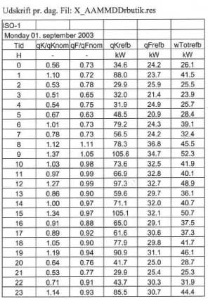
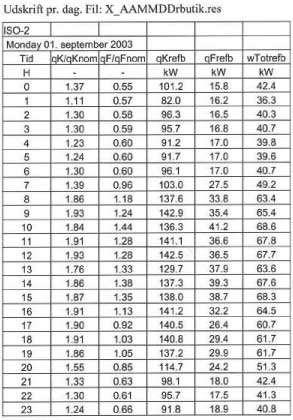
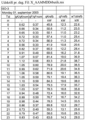
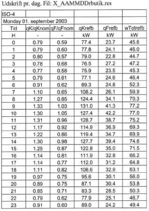
5 Daily printouts. File type X_AAMMDDrbutik.res

These files contain standardised refrigeration outputs and outputs and total power consumptions for reference shops based on scaling of appliance/store data

6 Printouts for the four shops

Click here to see: udskrift fra ISO 1 pr. måned - Fil: X_AAMMc.res

Click here to see: udskrift fra ISO 2 pr. måned - Fil: X_AAMMc.res

Click here to see: udskrift fra ISO 3 pr. måned - Fil: X_AAMMc.res

Click here to see: udskrift fra ISO 4 pr. måned - Fil: X_AAMMc.res

Click here to see: udskrift fra ISO 1 pr. time - Fil: X_AADDc.res

Click here to see: udskrift fra ISO 2 pr. time - Fil: X_AADDc.res

Click here to see: udskrift fra ISO 3 pr. time - Fil: X_AADDc.res

Click here to see: udskrift fra ISO 4 pr. time - Fil: X_AADDc.res

Click here to see: udskrift fra ISO 1 pr. dag - Fil: X_AADDfrugt.res

Click here to see: udskrift fra ISO 2 pr. dag - Fil: X_AADDfrugt.res

Click here to see: udskrift fra ISO 3 pr. dag - Fil: X_AADDfrugt.res

Click here to see: udskrift fra ISO 4 pr. dag - Fil: X_AADDfrugt.res

| Top | | Front page |

Version 1.0 September 2004, © Danish Environmental Protection Agency