Establishment of a basis for administrative use of PestSurf
Annex 3
3 Comparison of risk assessment data produced by spray drift assessments, FOCUS SW and PestSurf
3.1 Chemical characteristics of the compound
| Compound: | Bromoxynil |
| Dose: | 0.12 kg ai./ha |
| Spraying time: | 1. April |
| Crop: | Winter wheat |
| Dose: | 0.18 kg ai./ha |
| Spraying time: | 7. October |
| Crop: | Winter wheat |
Table 3.1. Overview of chemical properties of Bromxynil and the parameters used in the simulations.
Tabel 3.1. Oversigt over bromoxynils kemiske egenskaber og parametrene brugt i simuleringerne.
| Chemical property | Condition | Recalculated values | |||
| Cas-no. | 1689-84-5 | ||||
| Molecular weight | 276.9 | ||||
| Form (acid, basic, neutral) | acid | ||||
| pKa | 3.86 | ||||
| Water solubility | 90 µg/l | (distillled water) | |||
| log Kow | 1.31 | at pH | 2 | KowA- | 1.04 |
| log Kow | 1.04 | at pH | 7 | KowAH | 1.31 |
| log Kow | at pH | KowAH+ | |||
| Vapor pressure, Pa | 1.7 × 10⁻⁴ | 25°C | 318.7 (Boiling point) | vapor pressure, Pa, 20°C | 8.49 × 10⁻⁵ |
| Henry’s law constant | 5.3 × 10⁻⁴ Pa.m³. mol-1 | Recalculated value, dimensionless | 2.18 × 10⁻⁷ | ||
| Sorption properties in soil | |||||
| Freundlich exp | 0.8 | ||||
| Koc, l/kg | 183.6 | ||||
| DT50 in soil, days | 0.54 | ||||
| DT50water | 5.9 dage | PestSurf input | |||
| DT50sedment | None mentioned | ||||
| DT50water/sediment | 5.9 days | DT50, days | 5.9 | ||
| Sediment konc., µg/l | 80 (default in PestSurf) | ||||
| Hydrolysis | no hydrolysis | at pH 5 | (acid) | ||
| at pH 7 | (neutral) | ||||
| at pH 9 | (basic) | ||||
| Photolysis | |||||
| quantum yield | φ = 4.8 x 10⁻² ? | ||||
| Spectrum | λmax = 221.2, ε = 30343 l mol-1 cm-1 | ||||
| λmax = 221.2, ε = 30343 l mol-1 cm-1 λmax = 287, ε = 18302 l mol-1 cm-1 – The value 18302 is implemented for 295-300, and the value is reduced by a factor of 5 for the next wavelengths: |
|||||
| 295-300: 18302 | |||||
| 300-310: 3660; | |||||
| 320-330: 146; | |||||
| 330-340: 30 | |||||
| 340-350: 0 | |||||
| Other | DT 50 <10 h (2 major by-products) |
3.2 Concentrations generated drift
| Compound | Direct spray | FOCUS buffer zones | ||
| Ditch | Stream | Pond | ||
| [µg·l-1] | [µg·l-1] | [µg·l-1] | [µg·l-1] | |
| Spring application | 40.0 | 1.104 | 0.742 | 0.324 |
| Autumn app | 60.0 | 1.656 | 1.114 | 0.486 |
3.3 Concentrations generated by FOCUS SW
3.3.1 D3- Ditch
| Bromoxynil, spring appl. | Ditch, D3 | |||||||
| Water | Sediment | |||||||
| Date | PEC | Date | TWAEC | Date | PEC | Date | TWAEC | |
| [µg L-1] | [µg L-1] | [µg kg-1] | [µg kg-1] | |||||
| Global max | 04-apr-92 | 0.759 | 05-apr-92 | 0.306 | ||||
| 1 d | 05-apr-92 | 0.304 | 05-apr-92 | 0.561 | 06-apr-92 | 0.237 | 06-apr-92 | 0.294 |
| 2 d | 06-apr-92 | 0.034 | 06-apr-92 | 0.348 | 07-apr-92 | 0.178 | 06-apr-92 | 0.268 |
| 4 d | 08-apr-92 | 0.002 | 08-apr-92 | 0.179 | 09-apr-92 | 0.122 | 08-apr-92 | 0.22 |
| 7 d | 11-apr-92 | 0.001 | 11-apr-92 | 0.103 | 12-apr-92 | 0.084 | 11-apr-92 | 0.174 |
| Bromoxynil, autumn appl. | Ditch, D3 | |||||||
| Water | Sediment | |||||||
| Date | PEC | Date | TWAEC | Date | PEC | Date | TWAEC | |
| [µg L-1] | [µg L-1] | [µg kg-1] | [µg kg-1] | |||||
| Global max | 10-oct-92 | 1.143 | 11-oct-92 | 0.57 | ||||
| 1 d | 11-oct-92 | 0.767 | 11-oct-92 | 0.957 | 12-oct-92 | 0.488 | 12-oct-92 | 0.559 |
| 2 d | 12-oct-92 | 0.275 | 12-oct-92 | 0.736 | 13-oct-92 | 0.386 | 13-oct-92 | 0.531 |
| 4 d | 14-oct-92 | 0.021 | 14-oct-92 | 0.418 | 15-oct-92 | 0.267 | 14-oct-92 | 0.459 |
| 7 d | 17-oct-92 | 0.003 | 17-oct-92 | 0.242 | 18-oct-92 | 0.184 | 17-oct-92 | 0.374 |
3.3.2 D4 – Pond
| Bromoxynil, spring application | Pond, D4 | |||||||
| Water | Sediment | |||||||
| Date | PEC | Date | TWAEC | Date | PEC | Date | TWAEC | |
| [µg L-1] | [µg L-1] | [µg kg-1] | [µg kg-1] | |||||
| Global max | 18-apr-85 | 0.026 | 01-may-85 | 0.049 | ||||
| 1 d | 19-apr-85 | 0.024 | 19-apr-85 | 0.025 | 02-may-85 | 0.048 | 01-may-85 | 0.049 |
| 2 d | 20-apr-85 | 0.023 | 20-apr-85 | 0.024 | 03-may-85 | 0.047 | 01-may-85 | 0.049 |
| 4 d | 22-apr-85 | 0.021 | 22-apr-85 | 0.023 | 05-may-85 | 0.045 | 02-may-85 | 0.049 |
| 7 d | 25-apr-85 | 0.018 | 25-apr-85 | 0.021 | 08-may-85 | 0.041 | 03-may-85 | 0.048 |
| Bromoxynil, autumn appl. | Pond, D4 | |||||||
| Water | Sediment | |||||||
| Date | PEC | Date | TWAEC | Date | PEC | Date | TWAEC | |
| [µg L-1] | [µg L-1] | [µg kg-1] | [µg kg-1] | |||||
| Global max | 26-oct-85 | 0.039 | 08-nov-85 | 0.065 | ||||
| 1 d | 27-oct-85 | 0.036 | 27-oct-85 | 0.037 | 09-nov-85 | 0.065 | 09-nov-85 | 0.065 |
| 2 d | 28-oct-85 | 0.033 | 28-oct-85 | 0.036 | 10-nov-85 | 0.065 | 09-nov-85 | 0.065 |
| 4 d | 30-oct-85 | 0.029 | 30-oct-85 | 0.033 | 12-nov-85 | 0.064 | 10-nov-85 | 0.065 |
| 7 d | 02-nov-85 | 0.024 | 02-nov-85 | 0.03 | 15-nov-85 | 0.062 | 12-nov-85 | 0.065 |
3.3.3 D4 – Stream
| Bromoxynil, spring appl. | Stream, D4 | |||||||
| Water | Sediment | |||||||
| Date | PEC | Date | TWAEC | Date | PEC | Date | TWAEC | |
| [µg L-1] | [µg L-1] | [µg kg-1] | [µg kg-1] | |||||
| Global max | 18-apr-85 | 0.603 | 18-apr-85 | 0.029 | ||||
| 1 d | 19-apr-85 | 0 | 19-apr-85 | 0.041 | 19-apr-85 | 0.02 | 19-apr-85 | 0.024 |
| 2 d | 20-apr-85 | 0 | 20-apr-85 | 0.02 | 20-apr-85 | 0.015 | 20-apr-85 | 0.021 |
| 4 d | 22-apr-85 | 0 | 22-apr-85 | 0.01 | 22-apr-85 | 0.01 | 22-apr-85 | 0.017 |
| 7 d | 25-apr-85 | 0 | 25-apr-85 | 0.006 | 25-apr-85 | 0.007 | 25-apr-85 | 0.013 |
| Bromoxynil, autumn appl. | Stream, D4 | |||||||
| Water | Sediment | |||||||
| Date | PEC | Date | TWAEC | Date | PEC | Date | TWAEC | |
| [µg L-1] | [µg L-1] | [µg kg-1] | [µg kg-1] | |||||
| Global max | 26-oct-85 | 0.987 | 26-oct-85 | 0.176 | ||||
| 1 d | 27-oct-85 | 0.002 | 27-oct-85 | 0.286 | 27-oct-85 | 0.111 | 27-oct-85 | 0.152 |
| 2 d | 28-oct-85 | 0.001 | 28-oct-85 | 0.144 | 28-oct-85 | 0.08 | 28-oct-85 | 0.127 |
| 4 d | 30-oct-85 | 0 | 30-oct-85 | 0.072 | 30-oct-85 | 0.053 | 30-oct-85 | 0.098 |
| 7 d | 02-nov-85 | 0 | 02-nov-85 | 0.041 | 02-nov-85 | 0.037 | 02-nov-85 | 0.076 |
3.3.4 Conclusion – FOCUS SW
The highest concentration is generated in the ditch (D3) for the autumn application. It is caused by wind drift and the concentration becomes 1.14 µg/l. The same scenario shows the highest concentration in the sediment, 0.570 µg/kg. For all scenarios, the concentrations are lower than what is generated by the simpler assessments.
3.4 Concentrations generated by PestSurf
3.4.1 Sandy Catchment, stream
The distribution of concentrations were assessed in several steps. First, the maximum concentrations at each calculation point were listed, and the dates for the occurrence of the maximum were assessed. The points, for which the maximum value also represents a local maximum were selected for further analysis. The relevant values are listed in Table 3.2.
Table 3.2. Maximum concentrations (ng/l) of bromoxynil simulated for each calculation point in the sandy catchment.
Tabel 3.2. Maximumskoncentrationer (ng/l) af bromoxynil simuleret for hvert beregningspunkt i det sandede opland.
The pattern over time was dominated by drift for both applications and all calculation points, see Figure 3.1 to Figure 3.4.
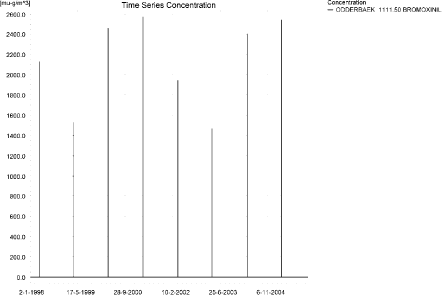
Figure 3.1. Concentration pattern over time for the spring application of bromoxynil in the sandy catchment, 1111.5 m from the upstream end.
Figur 3.1. Koncentrationsmønster som funktion af tid for forårsudbragt bromoxynil i det sandede opland, 1111.5 m fra den opstrøms ende.
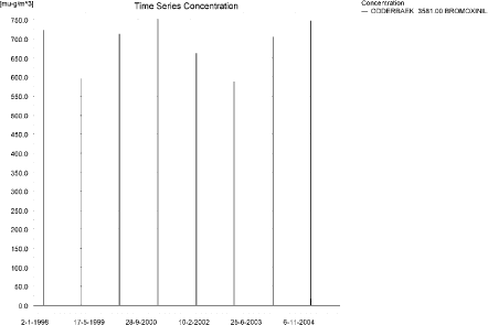
Figure 3.2. Concentration pattern over time for the spring application of bromoxynil in the sandy catchment, 3581 m from the upstream end.
Figur 3.2. Koncentrationsmønster som funktion af tid for bromoxynil i det sandede opland, 3581 m fra den opstrøms ende.
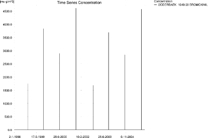
Figure 3.3. Concentration pattern over time for the autumn application of bromoxynil in the sandy catchment, 1049 m from the upstream end.
Figur 3.3. Koncentrationsmønster som funktion af tid for efterårsudbragt bromoxynil i det sandede opland, 1049 m fra den opstrøms ende.
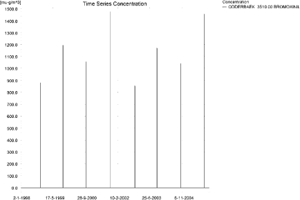
Figure 3.4. Concentration pattern over time for the autumn application of bromoxynil in the sandy catchment, 3510 m from the upstream end.
Figur 3.4. Koncentrationsmønster som funktion af tid for efterårsudbragt bromoxynil i det sandede opland, 3510 m fra den opstrøms ende.
Each of the drift-events generated an almost identical pattern along the stream, see Figure 3.5 and Figure 3.6. The thin black line represents the concentration, while the full black line shows the maximum concentrations obtained during the simulations. In addition, the outline of the stream is shown. In the middle of the catchment, the stream is protected by unsprayed areas.
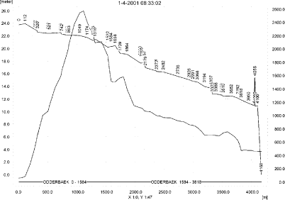
Figure 3.5. Concentrations of spring-applied bromoxynil in the sandy catchment on 1. April 2001, just after spraying.
Figur 3.5. Koncentrationer af forårsudbragt bromoxynil i det sandede opland den 1. april 2001, lige efter endt sprøjtning.
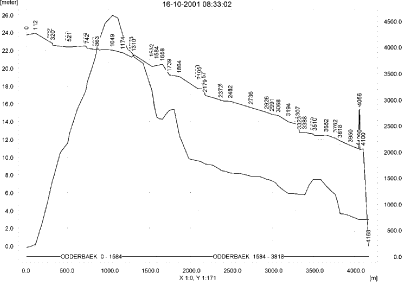
Figure 3.6. Concentrations of autumn-applied bromoxynil in the sandy catchment on 16. October 2001, just after spraying.
Figur 3.6. Koncentrationer af efterårsudbragt bromoxynil i det sandede opland den 16. oktober 2001, lige efter endt sprøjtning.
In order to present the data in a similar fashion to the FOCUS SW-results, data were extracted and recalculated for the time series marked in Table 3.2. The global maxima and time weighted concentrations (up to 7 days) were extracted and are reported in Table 3.3 and Table 3.4. Note that the unit is ng/l.
The concentrations of bromoxynil adsorbed to macrophytes for the spring application is shown in Figure 3.7 and Figure 3.8. The maximum concentration is 1.44 ng/l. For the autumn-application, the value only reaches 0.593 ng/l due to presence of fewer macrophytes at that time of the year. The concentration in the water phase is only marginally affected by macrophytes.
The amount of bromoxynil in porewater is shown in Figure 3.9 for the spring application and in Figure 3.10 for the autumn application. The maximum concentrations reached are 0.028 and 0.071 ng/l for the spring and autumn applications respectively, both values 1421 m from the upstream end. The corresponding max concentration in sediment is 0.59 ng/kg and 1.27 ng/kg.
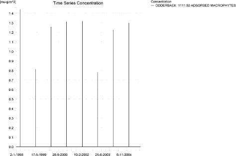
Figure 3.7. Macrophyte-bound concentration of spring-applied bromoxynilin the sandy catchment.
Figur 3.7. Koncentration af forårsudbragt bromoxynil på makrofytter i det sandede opland.
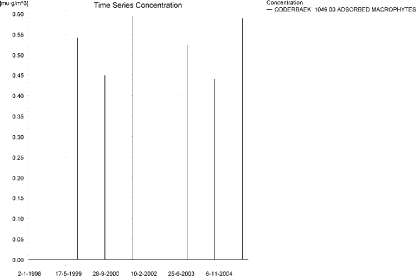
Figure 3.8. Macrophyte-bound concentration of Autumn-applied bromoxynil in the sandy catchment.
Figur 3.8. Koncentration af efterårsudbragt bromoxynil på makrofytter i det sandede opland.
Table 3.3. Concentration of spring-applied bromoxynil, ng/l, at selected points in the sandy stream.
Tabel 3.3. Koncentration af forårsudbragt bromoxynil, ng/l, på udvalgte lokaliteter i det sandede vandløb.
| Year | ODDERBAEK 1111.50 | ODDERBAEK 1801.50 | ODDERBAEK 3581.00 | |||||||
| Conc | TWC | Date | Conc. | TWC | Date | Conc. | TWC | Date | ||
| 1998 | (global max) | 2132 | 07-04-1998 | 1420 | 07-04-1998 | 723 | 07-04-1998 | |||
| 1 hour (after max) | 626 | 1328 | 924 | 1173 | 258 | 373 | ||||
| 1 day after sp.in. | 0 | 66 | 0 | 76 | 0 | 83 | ||||
| 2 days | 0 | 22 | 0 | 25 | 0 | 27 | ||||
| 4 days | 0 | 16 | 0 | 19 | 0 | 20 | ||||
| 7 days | 0 | 9 | 0 | 11 | 0 | 12 | ||||
| 1999 | (global max) | 1526 | 02-04-1999 | 1177 | 02-04-1999 | 596 | 02-04-1999 | |||
| 1 hour (after max) | 305 | 873 | 578 | 889 | 274 | 293 | ||||
| 1 day after sp.in. | 0 | 39 | 0 | 48 | 0 | 55 | ||||
| 2 days | 0 | 13 | 0 | 16 | 0 | 18 | ||||
| 4 days | 0 | 10 | 0 | 12 | 0 | 13 | ||||
| 7 days | 0 | 5 | 0 | 7 | 0 | 8 | ||||
| 2000 | (global max) | 2461 | 01-04-2000 | 1570 | 01-04-2000 | 713 | 01-04-2000 | |||
| 1 hour (after max) | 878 | 1644 | 1156 | 1346 | 223 | 361 | ||||
| 1 day after sp.in. | 0 | 86 | 0 | 99 | 0 | 86 | ||||
| 2 days | 0 | 28 | 0 | 32 | 0 | 28 | ||||
| 4 days | 0 | 21 | 0 | 24 | 0 | 21 | ||||
| 7 days | 0 | 12 | 0 | 14 | 0 | 12 | ||||
| 2001 | (global max) | 2570 | 01-04-2001 | 1581 | 01-04-2001 | 752 | 01-04-2001 | |||
| 1 hour (after max) | 956 | 1727 | 1179 | 1352 | 242 | 391 | ||||
| 1 day after sp.in. | 0 | 94 | 0 | 103 | 0 | 95 | ||||
| 2 days | 0 | 31 | 0 | 34 | 0 | 31 | ||||
| 4 days | 0 | 23 | 0 | 25 | 0 | 23 | ||||
| 7 days | 0 | 13 | 0 | 14 | 0 | 13 | ||||
| 2002 | (global max) | 1946 | 07-04-2002 | 1347 | 07-04-2002 | 663 | 07-04-2002 | |||
| 1 hour (after max) | 514 | 1183 | 816 | 1089 | 247 | 332 | ||||
| 1 day after sp.in. | 0 | 56 | 0 | 67 | 0 | 70 | ||||
| 2 days | 0 | 19 | 0 | 22 | 0 | 23 | ||||
| 4 days | 0 | 14 | 0 | 16 | 0 | 17 | ||||
| 7 days | 0 | 8 | 0 | 9 | 0 | 10 | ||||
| 2003 | (global max) | 1469 | 02-04-2003 | 1149 | 02-04-2003 | 587 | 02-04-2003 | |||
| 1 hour (after max) | 274 | 826 | 544 | 859 | 282 | 289 | ||||
| 1 day after sp.in. | 0 | 36 | 0 | 45 | 0 | 53 | ||||
| 2 days | 0 | 12 | 0 | 15 | 0 | 17 | ||||
| 4 days | 0 | 9 | 0 | 11 | 0 | 13 | ||||
| 7 days | 0 | 5 | 0 | 6 | 0 | 7 | ||||
| 2004 | (global max) | 2404 | 01-04-2004 | 1542 | 01-04-2004 | 706 | 01-04-2004 | |||
| 1 hour (after max) | 833 | 1593 | 1118 | 1316 | 223 | 356 | ||||
| 1 day after sp.in. | 0 | 83 | 0 | 95 | 0 | 84 | ||||
| 2 days | 0 | 27 | 0 | 31 | 0 | 28 | ||||
| 4 days | 0 | 20 | 0 | 23 | 0 | 21 | ||||
| 7 days | 0 | 12 | 0 | 13 | 0 | 12 | ||||
| 2005 | (global max) | 2544 | 01-04-2005 | 1566 | 01-04-2005 | 748 | 01-04-2005 | |||
| 1 hour (after max) | 934 | 1702 | 1160 | 1336 | 241 | 388 | ||||
| 1 day after sp.in. | 0 | 92 | 0 | 101 | 0 | 94 | ||||
| 2 days | 0 | 30 | 0 | 33 | 0 | 31 | ||||
| 4 days | 0 | 23 | 0 | 25 | 0 | 23 | ||||
| 7 days | 0 | 13 | 0 | 14 | 0 | 13 | ||||
| global max | 2570 | 0 | 1581 | 0 | 752 | 0 | ||||
| 1 hour | 956 | 1727 | 1179 | 1352 | 282 | 391 | ||||
| 1 day | 0 | 94 | 0 | 103 | 0 | 95 | ||||
| 2 days | 0 | 31 | 0 | 34 | 0 | 31 | ||||
| 4 days | 0 | 23 | 0 | 25 | 0 | 23 | ||||
| 7 days | 0 | 13 | 0 | 14 | 0 | 13 | ||||
Table 3.4. Concentration of autumn-applied bromoxynil, ng/l, at selected points in the sandy stream.
Tabel 3.4. Koncentration af efterårsudbragt bromoxynil, ng/l, på udvalgte lokaliteter i det sandede vandløb.
| Year | ODDERBAEK 1049.00 | ODDERBAEK 1801.50 | ODDERBAEK 3510.00 | |||||||
| Conc. | TWC | Date | Conc | TWC | Date | Conc. | TWC | Date | ||
| 1998 | (global max) | 1743 | 02-11-1998 | 1469 | 02-11-1998 | 879 | 02-11-1998 | |||
| 1 hour (after max) | 191 | 840 | 554 | 1030 | ||||||
| 1 day after sp.in. | 0 | 35 | 0 | 50 | 0 | 35 | ||||
| 2 days | 0 | 11 | 0 | 16 | 0 | 12 | ||||
| 4 days | 0 | 9 | 0 | 12 | 0 | 9 | ||||
| 7 days | 0 | 5 | 0 | 7 | 0 | 5 | ||||
| 1999 | (global max) | 3832 | 15-10-1999 | 2362 | 15-10-1999 | 1195 | 15-10-1999 | |||
| 1 hour (after max) | 1283 | 2466 | 1797 | 2025 | 418 | 620 | ||||
| 1 day after sp.in. | 0 | 130 | 0 | 158 | 0 | 167 | ||||
| 2 days | 0 | 43 | 0 | 52 | 0 | 55 | ||||
| 4 days | 0 | 32 | 0 | 39 | 0 | 41 | ||||
| 7 days | 0 | 18 | 0 | 22 | 0 | 23 | ||||
| 2000 | (global max) | 2894 | 14-10-2000 | 2077 | 14-10-2000 | 1055 | 14-10-2000 | |||
| 1 hour (after max) | 692 | 1704 | 1372 | 1737 | 416 | 533 | ||||
| 1 day after sp.in. | 0 | 80 | 0 | 110 | 0 | 128 | ||||
| 2 days | 0 | 26 | 0 | 36 | 0 | 42 | ||||
| 4 days | 0 | 20 | 0 | 27 | 0 | 31 | ||||
| 7 days | 0 | 11 | 0 | 15 | 0 | 18 | ||||
| 2001 | (global max) | 4609 | 16-10-2001 | 2813 | 16-10-2001 | 1475 | 16-10-2001 | |||
| 1 hour (after max) | 2312 | 3370 | 2272 | 2346 | 529 | 817 | ||||
| 1 day after sp.in. | 0 | 239 | 0 | 279 | 0 | 254 | ||||
| 2 days | 0 | 78 | 0 | 91 | 0 | 84 | ||||
| 4 days | 0 | 59 | 0 | 68 | 0 | 63 | ||||
| 7 days | 0 | 33 | 0 | 39 | 0 | 36 | ||||
| 2002 | (global max) | 1682 | 02-11-2002 | 1429 | 02-11-2002 | 856 | 02-11-2002 | |||
| 1 hour (after max) | 167 | 792 | 514 | 991 | ||||||
| 1 day after sp.in. | 0 | 33 | 0 | 47 | 0 | 32 | ||||
| 2 days | 0 | 11 | 0 | 15 | 0 | 11 | ||||
| 4 days | 0 | 8 | 0 | 12 | 0 | 8 | ||||
| 7 days | 0 | 5 | 0 | 7 | 0 | 5 | ||||
| 2003 | (global max) | 3694 | 15-10-2003 | 2307 | 15-10-2003 | 1171 | 15-10-2003 | |||
| 1 hour (after max) | 1186 | 2347 | 1723 | 1971 | 413 | 603 | ||||
| 1 day after sp.in. | 0 | 122 | 0 | 149 | 0 | 160 | ||||
| 2 days | 0 | 40 | 0 | 49 | 0 | 52 | ||||
| 4 days | 0 | 30 | 0 | 37 | 0 | 39 | ||||
| 7 days | 0 | 17 | 0 | 21 | 0 | 22 | ||||
| 2004 | (global max) | 2835 | 14-10-2004 | 2035 | 14-10-2004 | 1039 | 14-10-2004 | |||
| 1 hour (after max) | 660 | 1657 | 1317 | 1690 | 418 | 524 | ||||
| 1 day after sp.in. | 0 | 77 | 0 | 106 | 0 | 124 | ||||
| 2 days | 0 | 25 | 0 | 35 | 0 | 41 | ||||
| 4 days | 0 | 19 | 0 | 26 | 0 | 30 | ||||
| 7 days | 0 | 11 | 0 | 15 | 0 | 17 | ||||
| 2005 | (global max) | 4567 | 16-10-2005 | 2795 | 16-10-2005 | 1457 | 16-10-2005 | |||
| 1 hour (after max) | 2243 | 3316 | 2243 | 2327 | 521 | 807 | ||||
| 1 day after sp.in. | 0 | 232 | 0 | 269 | 0 | 249 | ||||
| 2 days | 0 | 76 | 0 | 88 | 0 | 82 | ||||
| 4 days | 0 | 57 | 0 | 66 | 0 | 61 | ||||
| 7 days | 0 | 32 | 0 | 38 | 0 | 35 | ||||
| Global max | 4609 | 2813 | 1475 | |||||||
| 1 hour (after max) | 2312 | 3370 | 2272 | 2346 | 529 | 817 | ||||
| 1 day after sp.in. | 0 | 239 | 0 | 279 | 0 | 254 | ||||
| 2 days | 0 | 78 | 0 | 91 | 0 | 84 | ||||
| 4 days | 0 | 59 | 0 | 68 | 0 | 63 | ||||
| 7 days | 0 | 33 | 0 | 39 | 0 | 36 | ||||
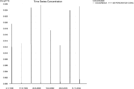
Figure 3.9. Example of Pore water concentration of spring-applied bromoxynil in the sandy catchment.
Figur 3.9. Porevandskoncentration for forårsudbragt bromoxynil i det sandede opland.
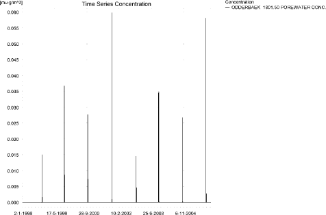
Figure 3.10. Example of Pore water concentration of autumn-applied bromoxynil in the sandy catchment.
Figur 3.10. Porevandskoncentration for efterårsudbragt bromoxynil i det sandede opland.
The global maximum value calculated by PestSurf for the sandy catchment in the water phase is 2.57 µg/l for the spring application and 4.61 µg/l for the autumn application. This is somewhat more than what is found in the D3-ditch scenario (0.759 and 1.143 µg/l for the spring and autumn-application, respectively). All maximum concentrations are reached through wind drift. The concentration in sediment in the D3-scenario is 0.31 and 0.57 µg/kg for the spring and autumn application, and thus much higher than the values calculated by Pestsurf.
Figure 3.11, Figure 3.12, Table 3.5 and Table 3.6 show the output of the PestSurf Excel template for the two applications of bromoxynil. The figure template works with pre-defined data extraction points. The plot requires specification of a “lowest detection value” (ldc) which defines when a pesticide occurrence is defined as an event. The time series plot is identical to the time series shown earlier, and the graph in the upper right corner resembles the plots in Figure 3.5 and Figure 3.6, but takes into account a longer period of time. A curve is generated when a downstream point reaches a concentration higher than the ldc. The programme then tracks the highest concentration for each calculation point in the stream within the last 24 hours. The plot in the lower right corner shows how many events have concentrations higher than a given toxicity value for the selected monitoring points. The curves are rather flat, showing little variation from year to year.
The tables shows part of the result sheet generated by the PestSurf Excel sheet based on the ldc-value. The selected table shows the point along the stream (of the pre-defined points) with the highest concentration.The highest concentration extracted by the PestSurf Excel sheet was 1.50 and 2.64 µg/l for the spring and autumn-simulation respectively. Thus, the pre-defined points have not caught the highest concentration of the simulation.
Click here to see Figure 3.11.
Figure 3.11. Overview for spring applied bromoxynil in the sandy catchment generated by the PestSurf excel template. The max concentrations generated over the 24 hours are similar to the overview in Figure 3.5. Detection value was set to 10 ng/l.
Figur 3.11. Oversigt for forårsudbragt bromoxynil i det sandede opland genereret med PestSurf-excel-skabelonen. Den maximale koncentration genereret over 24 timer svarer til oversigten i Figur 3.5. Detektionsgrænsen var sat til 10 ng/l.
Click here to see Figure 3.12.
Figure 3.12. Overview for autumn applied bromoxynil in the sandy catchment generated by the PestSurf excel template. The max concentrations generated over the 24 hours are similar to the overview in Figure 3.6. Detection value was set to 10 ng/l.
Figur 3.12. Oversigt for efterårsudbragt bromoxynil i det sandede opland genereret med PestSurf-excel-skabelonen. Den maximale koncentration genereret over 24 timer svarer til oversigten i Figur 3.5. Detektionsgrænsen var sat til 10 ng/l.
Table 3.5. Part of the result sheet generated by the PestSurf Excel sheet for the spring-application of bromoxynil. The selected table shows the point along the stream with the highest concentration recorded. Lowest detection value is set to 10 ng/l, toxicity to fish, daphnies and algae are set to 100, 1000 and 2000 ng/, respectively. The recorded peaks are shown in Figure 3.11.
Tabel 3.5. Uddrag af resultatpresentationen genereret af PestSurf-Excel-arket for forårsudbragt bromoxynil. Den udvalgte tabel viser det fordefinerede punkt langs med åen med højest koncentration. Detektionsgrænsen er sat til 10 mens toxicitetsværdierne for fisk, dafnier og alger er henholdsvis 100, 1000 og 2000 ng/l. De tabellerede hændelserne er vist i Figur 3.11.
Table 3.6. Part of the result sheet generated by the PestSurf Excel sheet for the autumn-application of bromoxynil. The selected table shows the point along the stream with the highest concentration recorded. The limiting values applied in the simulation is lowest detection valuε = 10 ng/l, toxicity to fish, daphnies and algae are set to 100, 1000 and 2000 ng/, respectively. The recorded peaks are shown in Figure 3.12.
Tabel 3.6. Uddrag af resultatpresentationen genereret af PestSurf-Excel-arket for efterårsudbragt bromoxynil. Den udvalgte tabel viser det fordefinerede punkt langs med åen med højest koncentration. Detektionsgrænsen er sat til 10 mens toxicitetsværdierne for fisk, dafnier og alger er henholdsvis 100, 1000 og 2000 ng/l. De tabellerede hændelserne er vist i Figur 3.11.
3.4.2 Sandy Catchment, pond
The concentration pattern is evaluated in the middle of the pond only, see Figure 3.13 and Figure 3.14. The pond receives drift and a contribution from groundwater. The drift peaks are just visible at the shown scale. The baseflow contribution is dominating the picture. The concentrations reached from a spring and and autumn application are almost identical, 0.311 and 0.462 µg/l, respectively. The peaks are caused by two different mechanisms. For the spring application, drainage causes the main peaks to occur. For the autumn application, the two highest peaks are caused by drift. The autumn is unusually dry this year and the water level in the pond is 10 cm at the time of spraying. The second highest peaks are caused by drainage. In both the spring and the autumn drainage case, rain occurs soon after spraying.
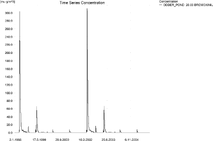
Figure 3.13. Concentrations of spring-applied bromoxynil in the sandy pond.
Figur 3.13. Koncentration af forårsudbragt bromoxynil i det sandede vandhul.
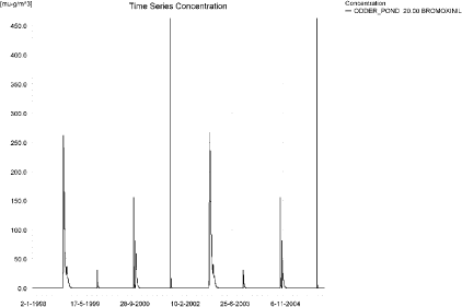
Figure 3.14. Concentrations of autumn-applied bromoxynil in the sandy pond.
Figur 3.14. Koncentration af efterårsudbragt bromoxynil i det sandede vandhul.
Table 3.7. Maximum concentrations of bromoxynil (ng/l) generated by drift and baseflow for the sandy pond for spring and autumn applications.
Tabel 3.7. Maximumskoncentrationer af bromoxynil (ng/l) genereret af drift og grundvandstilstrømning for det sandede vandhul for forårs- og efterårsudbringning.
| Year | Spring application | Autumn application | |||||
| Conc. | TWC | Date | Conc. | TWC | Date | ||
| 1998 | (global max) | 303 | 18-04-1998 | 261 | 12-11-1998 | ||
| 1 hour (after max) | 261 | 261 | |||||
| 1 day after sp.in. | 295 | 298 | 256 | 260 | |||
| 2 days | 257 | 283 | 230 | 247 | |||
| 4 days | 240 | 275 | 225 | 242 | |||
| 7 days | 193 | 249 | 173 | 223 | |||
| 1999 | (global max) | 65 | 18-04-1999 | 31 | 15-10-1999 | ||
| 1 hour (after max) | 24 | 25 | |||||
| 1 day after sp.in. | 64 | 65 | 17 | 20 | |||
| 2 days | 56 | 62 | 12 | 16 | |||
| 4 days | 51 | 60 | 10 | 15 | |||
| 7 days | 43 | 54 | 6 | 12 | |||
| 2000 | (global max) | 7 | 01-04-2000 | 155 | 14-10-2000 | ||
| 1 hour (after max) | 5 | 6 | 126 | 135 | |||
| 1 day after sp.in. | 5 | 5 | 54 | 78 | |||
| 2 days | 4 | 4 | 23 | 50 | |||
| 4 days | 3 | 4 | 16 | 42 | |||
| 7 days | 2 | 4 | 6 | 28 | |||
| 2001 | (global max) | 7 | 01-04-2001 | 462 | 16-10-2001 | ||
| 1 hour (after max) | 5 | 6 | 305 | 358 | |||
| 1 day after sp.in. | 5 | 5 | 76 | 134 | |||
| 2 days | 4 | 4 | 22 | 74 | |||
| 4 days | 3 | 4 | 12 | 59 | |||
| 7 days | 2 | 4 | 2 | 36 | |||
| 2002 | (global max) | 311 | 18-04-2002 | 267 | 12-11-2002 | ||
| 1 hour (after max) | 311 | 311 | 267 | 267 | |||
| 1 day after sp.in. | 303 | 306 | 257 | 265 | |||
| 2 days | 265 | 291 | 236 | 251 | |||
| 4 days | 248 | 282 | 231 | 247 | |||
| 7 days | 201 | 257 | 178 | 228 | |||
| 2003 | (global max) | 66 | 18-04-2003 | 31 | 15-10-2003 | ||
| 1 hour (after max) | 66 | 66 | 24 | 25 | |||
| 1 day after sp.in. | 65 | 66 | 17 | 20 | |||
| 2 days | 57 | 63 | 12 | 16 | |||
| 4 days | 52 | 61 | 10 | 15 | |||
| 7 days | 44 | 55 | 6 | 12 | |||
| 2004 | (global max) | 7 | 01-04-2004 | 155 | 14-10-2004 | ||
| 1 hour (after max) | 5 | 6 | 126 | 135 | |||
| 1 day after sp.in. | 5 | 5 | 54 | 78 | |||
| 2 days | 4 | 4 | 23 | 50 | |||
| 4 days | 3 | 4 | 16 | 42 | |||
| 7 days | 2 | 4 | 6 | 28 | |||
| 2005 | (global max) | 7 | 01-04-2005 | 462 | 16-10-2005 | ||
| 1 hour (after max) | 5 | 6 | 305 | 358 | |||
| 1 day after sp.in. | 5 | 5 | 76 | 134 | |||
| 2 days | 4 | 4 | 22 | 74 | |||
| 4 days | 3 | 4 | 12 | 59 | |||
| 7 days | 2 | 4 | 2 | 36 | |||
| Global max | 311 | 462 | |||||
| 1 hour (after max) | 311 | 311 | 305 | 358 | |||
| 1 day after sp.in. | 303 | 306 | 257 | 265 | |||
| 2 days | 265 | 291 | 236 | 251 | |||
| 4 days | 248 | 282 | 231 | 247 | |||
| 7 days | 201 | 257 | 178 | 228 | |||
The sorption to macrophytes is shown in Figure 3.15 and Figure 3.16. The maximum sorption is 0.27 and 0.35 ng/l, respectively, which is negligible compared to the concentration in the water phase. The max. concentrations reached for pore water concentration was 0.20 and 1.18 ng/l for the spring and autumn-application, respectively, see Figure 3.17 and Figure 3.19. No significant amounts were adsorbed to sediment, as shown in Figure 3.18 and Figure 3.20. The resulting sediment concentrations become 1.2 and 7.1 ng/kg, respectively.
Compared to the FOCUS D3-ditch, the concentration in the PestSurf sandy pond is slightly lower, 0.311 µg/l compared to 0.759 µg/l – for the spring-application and 0.462 µg/l compared to 1.143 µg/l for the autumn-application. In the pond-case, there is no difference between the results of PestSurf and the results extracted by the templates.
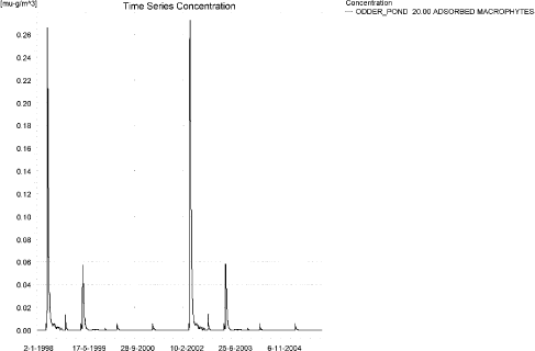
Figure 3.15. Sorption of spring-applied bromoxynil to macrophytes in the sandy pond.
Figur 3.15. Sorption af forårsudbragt bromoxynil til makrofytter i det sandede vandhul.
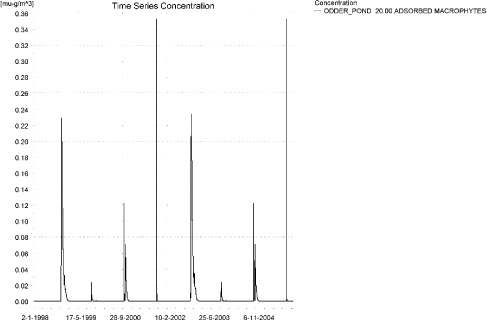
Figure 3.16. Sorption of autumn-applied bromoxynil to macrophytes in the sandy pond.
Figur 3.16. Sorption af efterårsudbragt bromoxynil til makrofytter i det sandede vandhul.
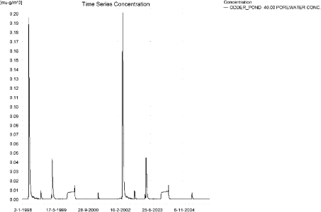
Figure 3.17. Pore water concentration of spring-applied bromoxynil in the sandy pond.
Figur 3.17. Porevandskoncentration af forårsudbragt bromoxynil i det sandede vandhul.
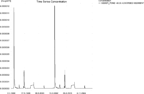
Figure 3.18. Sorption of spring-applied bromoxynil to sediment in the sandy pond. The concentration is in µg/g sediment and not µg/m³ as stated.
Figur 3.18. Sorption af forårsudbragt bromoxynil på sediment i det sandede vandhul. Koncentrationen er i µg/g sediment og ikke µg/m³ som angivet.
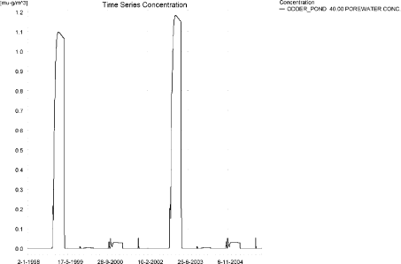
Figure 3.19. Pore water concentration of autumn-applied bromoxynil in the sandy pond.
Figur 3.19. Porevandskoncentration af efterårsudbragt bromoxynil i det sandede vandhul.
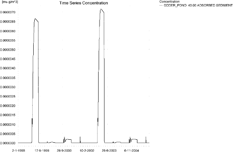
Figure 3.20. Sorption of autumn-applied bromoxynil to sediment in the sandy pond. The concentration is in µg/g sediment and not µg/m³ as stated.
Figur 3.20. Sorption af efterårsårsudbragt bromoxynil på sediment i det sandede vandhul. Koncentrationen er i µg/g sediment og ikke µg/m³ som angivet.
Click here to see Figure 3.21.
Figure 3.21. Overview for spring-applied bromoxynil in the sandy pond generated by the PestSurf excel template. The time series shown is identical to the one in Figure 3.13. The lowest detection value is 0.1 ng/l.
Figur 3.21. Oversigt for forårsudbragt bromoxynil i det sandede vandhul genereret med PestSurf-excel-skabelonen. Den viste tidsserie er mage til den i Figur 3.13. Detektionsgrænsen er sat til 0.1 ng/l.
Click here to see Figure 3.22.
Figure 3.22. Overview for autumn-applied bromoxynil in the sandy pond generated by the PestSurf excel template.. The time series shown is identical to the one in Figure 3.14. The lowest detection value is 0.1 ng/l.
Figur 3.22. Oversigt for efterårsudbragt bromoxynil i det sandede vandhul genereret med PestSurf-excel-skabelonen. Den viste tidsserie er mage til den i Figur 3.13. Detektionsgrænsen er sat til 0.1 ng/l.
Table 3.8. Part of the result sheet generated by the PestSurf Excel sheet, applied to the spring application of bromoxynil. The limiting value used for generation of the table is 0.1 ng/l. Lowest effect value for fish, daphnies and algaes were set to 1, 10 and 100 ng/l, respectively. The recorded peaks are shown in Figure 3.21.
Tabel 3.8. Uddrag af resultatpresentationen genereret af PestSurf-Excel-arket. Grænseværdien anvendt til generering af tabellen er 0.1 ng/l mens toxicitetsværdierne for fisk, dafnier og alger er henholdsvis 1, 10 og 100 ng/l. De tabellerede hændelser er vist i Figur 3.21.
Table 3.9. Part of the result sheet generated by the PestSurf Excel sheet, applied to the autumn application of bromoxynil. The limiting value used for generation of the table is 0.1 ng/l. Lowest effect value for fish, daphnies and algaes were set to 1, 10 and 100 ng/l, respectively. The recorded peaks are shown in Figure 3.22.
Tabel 3.9. Uddrag af resultatpresentationen genereret af PestSurf-Excel-arket. Grænseværdien anvendt til generering af tabellen er 0.1 ng/l mens toxicitetsværdierne for fisk, dafnier og alger er henholdsvis 1, 10 og 100 ng/l. De tabellerede hændelser er vist i Figur 3.21.
3.4.3 Sandy Loam Catchment, stream
The distribution of concentrations was assessed in several steps. First, the maximum concentrations at each calculation point were listed, and the dates for the occurrence of the maximum was assessed. The points, for which the maximum value also represents a local maximum were selected for further analysis. The relevant values are listed in Table 3.10.
All maximum values are caused by drift and are due to the assumption that all agricultural land is sprayed within 30 minutes. The maximum values are reached during a period with low flow in the stream. To illustrate that the level of magnitude is correct, the following calculation can be carried out: The amount sprayed for the spring application is 0.12 kg a.s./ha, equal to 12 µg/m². With a buffer zone of 1.5 m, 2.11 % reaches the stream. This equals 0.253 µg/m². The water depth between Ovrelillebaek 0 and 250 m varies between 3.5 and 6 cm, increasing to 8.5 at 300 m and 16.5 cm at the end of the stream. 0.253 µg/m² / 0.06 m equals 4.2 µg/l. The maximum values reached further downstream occurs when water, already loaded with pesticide, continues to receive drift. For 7.10. 1997, the water levels are about half of these values and the dosage is higher. The cross section in the upstream end is triangular.
Time series for the spring application are shown in Figure 3.23 and Figure 3.24, and for the autumn application in Figure 3.25 and Figure 3.26.
Table 3.10. Maximum concentrations (ng/l) of bromoxynil simulated for each calculation point in the sandy loam catchment, for spring and autumn applications respectively.
Tabel 3.10. Maximumskoncentrationer (ng/l) af bromoxynil simuleret for hvert beregningspunkt i morænelersoplandet, for henholdsvis forårs- og efterårsudbringingen.
| BROMOXYNIL | Spring Application | Autumn Application | ||||
| Maximum | Max.Time | Local Maxima | Maximum | Max.Time | Local Maxima | |
| ALBJERGBAEK 0.00 | 4 | 02-04-1996 20:00 | 1 | 09-10-2001 15:00 | ||
| ALBJERGBAEK 150.00 | 7 | 03-04-1996 05:00 | 1 | 09-10-2001 16:00 | ||
| ALBJERGBAEK 300.00 | 5 | 05-04-1996 20:00 | 5 | 07-10-1994 09:09 | ||
| ALBJERGBAEK 450.00 | 5 | 05-04-1996 21:00 | 1 | 09-10-2001 21:00 | ||
| ALBJERGBAEK 600.00 | 2076 | 31-03-2000 09:00 | 4012 | 07-10-1997 12:00 | ||
| ELHOLTBAEK 0.00 | 4 | 31-03-2001 09:00 | 8 | 07-10-1995 09:19 | ||
| ELHOLTBAEK 165.00 | 2 | 02-04-1996 20:00 | 0 | 08-10-2001 05:00 | ||
| ELHOLTBAEK 330.00 | 1652 | 31-03-2001 08:40 | 3347 | 07-10-1997 08:49 | ||
| FREDLIGBAEK 0.00 | 2 | 02-04-1996 18:00 | 0 | 09-10-2001 03:00 | ||
| FREDLIGBAEK 100.00 | 3 | 02-04-1996 18:00 | 0 | 30-10-1998 16:00 | ||
| FREDLIGBAEK 200.00 | 3 | 02-04-1996 18:00 | 0 | 30-10-1998 04:00 | ||
| FREDLIGBAEK 300.00 | 3 | 02-04-1996 18:00 | 0 | 30-10-1998 04:00 | ||
| FREDLIGBAEK 400.00 | 3 | 02-04-1996 18:00 | 0 | 30-10-1998 04:00 | ||
| FREDLIGBAEK 500.00 | 3 | 02-04-1996 18:00 | 0 | 30-10-1998 04:00 | ||
| FREDLIGBAEK 600.00 | 7 | 01-04-1998 00:40 | 7 | 07-10-1994 09:00 | ||
| FREDLIGBAEK 667.50 | 3 | 02-04-1996 19:00 | 3 | 10-10-1997 11:00 | ||
| FREDLIGBAEK 735.00 | 3440 | 31-03-2000 08:40 | x | 6199 | 07-10-1995 09:10 | |
| GROFTEBAEK 0.00 | 1 | 02-04-1996 17:00 | 0 | 11-10-1997 02:00 | ||
| GROFTEBAEK 155.00 | 3 | 02-04-1996 17:00 | 1 | 09-10-2001 21:00 | ||
| GROFTEBAEK 310.00 | 11 | 31-03-2000 09:19 | 13 | 07-10-1996 09:00 | ||
| GROFTEBAEK 465.00 | 2 | 02-04-1996 14:00 | 0 | 31-10-1998 07:00 | ||
| GROFTEBAEK 620.00 | 2845 | 31-03-2000 08:40 | 8240 | 07-10-1997 09:00 | x | |
| STENSBAEK 0.00 | 9 | 02-04-1996 17:00 | 142 | 09-10-2001 04:00 | ||
| STENSBAEK 125.00 | 14 | 03-04-1996 05:00 | 111 | 09-10-2001 05:00 | ||
| STENSBAEK 250.00 | 4 | 02-04-1996 18:00 | 47 | 09-10-2001 06:00 | ||
| STENSBAEK 412.50 | 4 | 02-04-1996 19:00 | 32 | 09-10-2001 07:00 | ||
| STENSBAEK 575.00 | 700 | 31-03-2000 09:19 | 2468 | 07-10-1997 14:00 | ||
| OVRELILLEBAEK 0.00 | 5 | 02-04-1996 22:00 | 0 | 11-12-2001 00:00 | ||
| OVRELILLEBAEK 125.00 | 4447 | 31-03-2000 08:30 | 6638 | 07-10-1995 08:30 | ||
| OVRELILLEBAEK 250.00 | 3490 | 31-03-2000 08:30 | 7188 | 07-10-1997 08:49 | ||
| OVRELILLEBAEK 290.00 | 5037 | 31-03-2000 08:30 | x | 9334 | 07-10-1996 10:00 | x |
| OVRELILLEBAEK 330.00 | 2076 | 31-03-2000 09:00 | 4012 | 07-10-1997 12:00 | ||
| OVRELILLEBAEK 330.00 | 2076 | 31-03-2000 09:00 | 4012 | 07-10-1997 12:00 | ||
| OVRELILLEBAEK 352.50 | 2632 | 31-03-2000 09:10 | 5296 | 07-10-1995 12:00 | ||
| OVRELILLEBAEK 375.00 | 700 | 31-03-2000 09:19 | 2468 | 07-10-1997 14:00 | ||
| OVRELILLEBAEK 375.00 | 700 | 31-03-2000 09:19 | 2468 | 07-10-1997 14:00 | ||
| OVRELILLEBAEK 437.50 | 776 | 31-03-2001 09:10 | 4142 | 07-10-1997 08:30 | ||
| OVRELILLEBAEK 500.00 | 1590 | 31-03-2000 08:30 | 6781 | 07-10-1997 08:30 | ||
| OVRELILLEBAEK 625.00 | 3132 | 31-03-2000 08:30 | x | 7735 | 07-10-1996 08:39 | |
| OVRELILLEBAEK 750.00 | 2046 | 31-03-2000 08:30 | 5100 | 07-10-1997 08:30 | ||
| OVRELILLEBAEK 855.00 | 2725 | 31-03-2000 08:30 | 7410 | 07-10-1997 08:30 | ||
| OVRELILLEBAEK 960.00 | 1652 | 31-03-2001 08:40 | 3347 | 07-10-1997 08:49 | ||
| OVRELILLEBAEK 960.00 | 1652 | 31-03-2001 08:40 | 3347 | 07-10-1997 08:49 | ||
| OVRELILLEBAEK 980.00 | 1751 | 31-03-2000 08:40 | 3580 | 07-10-1997 08:49 | ||
| OVRELILLEBAEK 1000.00 | 1456 | 31-03-2001 08:40 | 2964 | 07-10-1997 09:00 | ||
| OVRELILLEBAEK 1062.50 | 1481 | 31-03-2001 08:49 | 2838 | 07-10-1997 09:00 | ||
| OVRELILLEBAEK 1125.00 | 1379 | 31-03-2001 08:49 | 3797 | 07-10-1997 08:30 | ||
| OVRELILLEBAEK 1187.50 | 1579 | 31-03-2000 08:30 | 4956 | 07-10-1997 08:30 | ||
| OVRELILLEBAEK 1250.00 | 1525 | 31-03-2000 08:30 | 6032 | 07-10-1997 08:30 | ||
| OVRELILLEBAEK 1425.00 | 2211 | 31-03-2000 08:30 | x | 7287 | 07-10-1997 08:30 | x |
| OVRELILLEBAEK 1600.00 | 1905 | 31-03-2000 08:30 | 5690 | 07-10-1997 08:30 | ||
| OVRELILLEBAEK 1650.00 | 2316 | 31-03-2000 08:30 | 7038 | 07-10-1997 08:40 | ||
| OVRELILLEBAEK 1700.00 | 1829 | 31-03-2000 08:40 | 4074 | 07-10-1997 09:19 | ||
| NEDRELILLEBAEK 0.00 | 1829 | 31-03-2000 08:40 | 4074 | 07-10-1997 09:19 | ||
| NEDRELILLEBAEK 135.00 | 1987 | 31-03-2000 08:30 | 4187 | 07-10-1997 08:30 | ||
| NEDRELILLEBAEK 270.00 | 2587 | 31-03-2000 08:30 | 7046 | 07-10-1997 08:30 | ||
| NEDRELILLEBAEK 330.00 | 3132 | 31-03-2000 08:30 | 8015 | 07-10-1997 08:30 | ||
| NEDRELILLEBAEK 390.00 | 3155 | 31-03-2000 08:30 | 7119 | 07-10-1997 08:40 | ||
| NEDRELILLEBAEK 495.50 | 4391 | 31-03-2000 08:30 | x | 8448 | 07-10-1995 08:40 | x |
| NEDRELILLEBAEK 601.00 | 3440 | 31-03-2000 08:40 | 6199 | 07-10-1995 09:10 | ||
| NEDRELILLEBAEK 601.00 | 3440 | 31-03-2000 08:40 | 6199 | 07-10-1995 09:10 | ||
| NEDRELILLEBAEK 693.00 | 3454 | 31-03-2000 08:49 | 6011 | 07-10-1996 09:50 | ||
| NEDRELILLEBAEK 785.00 | 3286 | 31-03-2000 09:00 | 9696 | 07-10-1997 08:30 | ||
| NEDRELILLEBAEK 847.00 | 4120 | 31-03-2000 08:30 | x | 13367 | 07-10-1997 08:30 | x |
| NEDRELILLEBAEK 909.00 | 2845 | 31-03-2000 08:40 | 8240 | 07-10-1997 09:00 | ||
| NEDRELILLEBAEK 909.00 | 2845 | 31-03-2000 08:40 | 8240 | 07-10-1997 09:00 | ||
| NEDRELILLEBAEK 984.50 | 2808 | 31-03-2000 09:19 | 7601 | 07-10-1997 09:19 | ||
| NEDRELILLEBAEK 1060.00 | 3409 | 31-03-2000 08:30 | 10891 | 07-10-1997 08:30 | ||
| NEDRELILLEBAEK 1169.50 | 4220 | 31-03-2000 08:30 | 13147 | 07-10-1997 08:30 | ||
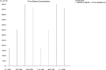
| NEDRELILLEBAEK 1279.00 | 6000 | 31-03-2000 08:30 | x | 17805 | 07-10-1997 08:40 | x |
| NEDRELILLEBAEK 1409.50 | 4954 | 31-03-2000 08:40 | 8586 | 07-10-1996 09:09 | ||
| NEDRELILLEBAEK 1540.00 | 3541 | 31-03-2000 09:19 | 5512 | 07-10-1996 11:00 | ||
| Global max | 6000 | 17805 | ||||
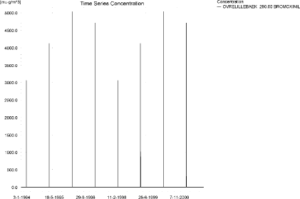
Figure 3.23. Concentration pattern for the spring application of bromoxynil in the upstream end of the sandy loam catchment, 290 m from the upstream end.
Figur 3.23. Koncentrationsmønster for forårsudbragt bromoxynil i den opstrøms ende af morænelersoplandet, 290 m fra den opstrøms ende.
< /p>
/p>
Figure 3.24. Concentration pattern for the spring application of bromoxynil in the lower end of the sandy loam catchment.
Figur 3.24. Koncentrationsmønster for forårsudbragt bromoxynil i den opstrøms ende af morænelersoplandet, 290 m fra den opstrøms ende.
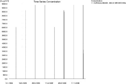
Figure 3.25. Concentration pattern for the autumn application of bromoxynil in the upstream end of the sandy loam catchment.
Figur 3.25. Koncentrationsmønster for efterårsudbragt bromoxynil i den opstrøms ende af morænelersoplandet.
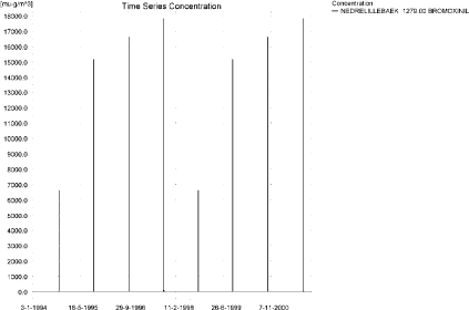
Figure 3.26. Concentration pattern for the autumn application of bromoxynil in the downstream end of the sandy loam catchment.
Figur 3.26. Koncentrationsmønster for efterårsudbragt bromoxynil i den nedstrøms ende af morænelersoplandet.
The longitudinal profile of the concentrations in the sandy loam catchment is shown in Figure 3.27 for the spring-application and Figure 3.28 for the autumn-application, respectively. The thin black line represents the concentration, while the thick black line shows the maximum concentrations obtained during the simulations. In addition, the outline of the stream is shown.
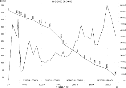
Figure 3.27. Concentrations in the sandy loam catchment on 31. March 2000 after spring applications. The concentrations are generated by wind drift.
Figur 3.27. Koncentrationer i morænelersoplandet den 31 marts-2000. efter forårsudbringning. Koncentrationerne genereres af vinddrift.
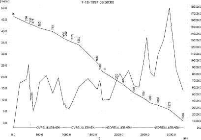
Figure 3.28. Concentrations in the sandy loam catchment on 7.October 1997 after autumn application.
Figur 3.28. Koncentrationer i morænelersoplandet den 7. oktober-1997. efter efterårsårsudbringning.
To be able to extract comparable values to FOCUS SW, the global maxima and time weighted concentrations (up to 7 days) were extracted when these were meaningful.
Figure 3.29 to Figure 3.32 show the concentrations sorbed to macrophytes, which had a maximum of 14 ng/l and 25 ng/l for the spring and autumn-application, respectively. The pattern follows the pattern of the water concentrations. The concentrations are insignificant compared to the concentrations in the water phase.
Figure 3.33 and Figure 3.34 show the concentration of bromoxynil in porewater at the place of maximum concentration. Figure 3.35 and Figure 3.36 show the corresponding concentration of bromoxynil adsorbed to sediment. The concentrations are quite low, 2.8 and 7.3 ng/kg, respectively.

Figure 3.29. Concentration on macrophytes in ng/l in the upper part of the sandy loam catchment (290 m from the upstream end) after spring application of bromoxynil.
Figur 3.29. Koncentration på makrofytter 290 m fra opstrøms ende af morænelersoplandet efter forårsudbringning af bromoxynil.
Figure 3.30. Concentration on macrophytes near the bottom of the sandy loam catchment after spring application of bromoxynil.
Figur 3.30. Koncentration på makrofytter nær udløbet fra morænelersoplandet efter forårsudbringning af bromoxynil.
Figure 3.31. Concentration on macrophytes in ng/l in the upper part of the sandy loam catchment after autumn application of bromoxynil (290 m from the upstream end).
Figur 3.31. Koncentration på makrofytter 290 m fra opstrøms ende af morænelersoplandet efter efterårsudbringning af bromoxynil.
Figure 3.32. Concentration on macrophytes in at the end of the sandy loam catchment after autumn application of bromoxynil.
Figur 3.32. Koncentration på makrofytter nær udløbet fra morænelersoplandet efter efterårsudbringning af bromoxynil.
Figure 3.33. Pore water concentration of spring-applied bromoxynil in the sandy loam catchment.
Figur 3.33. Porevandskoncentration af forårsudbragt bromoxynil i morænelersoplandet.
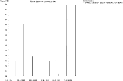
Figure 3.34. Pore water concentration of autumn-applied bromoxynil in the sandy loam catchment.
Figur 3.34. Porevandskoncentration af efterårsudbragt bromoxynil i morænelersoplandet.

Figure 3.35. Sediment concentration of spring-applied bromoxynil in the sandy loam catchment. Note that the concentration is in µg/g sediment and not µg/m² as indicated.
Figur 3.35. sedimentkoncentrations for forårsudbragt bromoxynil i morænelersoplandet. Bemærk at koncentrationen er i µg/g sediment og ikke µg/m³ som angivet.
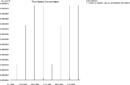
Figure 3.36. Sediment concentration of autumn-applied bromoxynil in the sandy loam catchment. Note that the concentration is in µg/g sediment and not µg/m² as indicated.
Figur 3.36. sedimentkoncentrations for efterårsudbragt bromoxynil i morænelersoplandet. Bemærk at koncentrationen er i µg/g sediment og ikke µg/m³ som angivet.
The FOCUS SW-D4 stream-scenario generates concentrations of 0.603 and 0.987 µg/l, for spring and autumn applications, respectively. PestSurf generates concentrations of 6.00 and 17.8 µg/l for the same applications. The difference in water depth account for a factor 2-5 and 3.5-10, respectively, and the contribution from the whole catchment explains the rest of the difference between the two models. The sediment concentrations are much lower in PestSurf, 3 and 7 ng/kg compared to 29 and 176 ng/kg in FOCUS for the two application times, respectively.
In comparison, drainage events resulted, at maximum, in concentrations of 14 and 142 ng/l, in both cases caused by rainfall occurring just after spraying.
Figure 3.37 to Figure 3.40 and Table 3.13 to Table 3.16 show the results as generated by the PestSurf templates. The maximum value generated by the templates for the upper part of the stream is 2.32 and 7.04 µg/l for the spring and the autumn-application, respectively, and for the lower part, 6.00 and 17.8 µg/l, respectively. In this case, the templates thus catch the actual maximum values simulated.
Table 3.11. Maximum concentrations (ng/l) of spring-applied bromoxynil simulated for selected calculation point in the sandy loam catchment.
Tabel 3.11. Maximum-koncentrationer (ng/l) af forårsudbragt bromoxynil beregnet for udvalgte lokaliteter i morænelersoplandet.
| Year | FREDLIGBAEK 735.00 | OVRELILLEBAEK 290.00 | OVRELILLEBAEK 625.00 | OVRELILLEBAEK 1425.00 | |||||||||
| Conc. | TWA | Date | Conc. | TWA | Date | Conc. | TWA | Date | Conc. | TWA | Date | ||
| 1994 | 1994 (global max) | 1143 | 02-04-1994 | 3060 | 02-04-1994 | 763 | 02-04-1994 | 876 | 02-04-1994 | ||||
| 1 hour (after max) | 333 | 664 | 495 | 1566 | 165 | 306 | 116 | 485 | |||||
| 1 day after sp.in. | 0 | 35 | 0 | 80 | 0 | 17 | 0 | 26 | |||||
| 2 days | 0 | 11 | 0 | 26 | 0 | 6 | 0 | 9 | |||||
| 4 days | 0 | 9 | 0 | 20 | 0 | 4 | 0 | 6 | |||||
| 7 days | 0 | 5 | 0 | 11 | 0 | 2 | 0 | 4 | |||||
| 1995 | 1995 (global max) | 2135 | 01-04-1995 | 4119 | 01-04-1995 | 1463 | 01-04-1995 | 1438 | 01-04-1995 | ||||
| 1 hour (after max) | 731 | 1258 | 1813 | 2954 | 305 | 505 | 595 | 1008 | |||||
| 1 day after sp.in. | 0 | 88 | 1 | 335 | 0 | 45 | 0 | 55 | |||||
| 2 days | 0 | 29 | 0 | 110 | 0 | 15 | 0 | 18 | |||||
| 4 days | 0 | 21 | 0 | 82 | 0 | 11 | 0 | 13 | |||||
| 7 days | 0 | 12 | 0 | 47 | 0 | 6 | 0 | 8 | |||||
| 1996 | 1996 (global max) | 3439 | 01-04-1996 | 5036 | 01-04-1996 | 3132 | 01-04-1996 | 2211 | 01-04-1996 | ||||
| 1 hour (after max) | 1423 | 2281 | 2208 | 3692 | 401 | 1423 | 1103 | 1335 | |||||
| 1 day after sp.in. | 1 | 147 | 7 | 578 | 4 | 158 | 1 | 99 | |||||
| 2 days | 1 | 49 | 0 | 191 | 1 | 53 | 1 | 34 | |||||
| 4 days | 1 | 37 | 0 | 143 | 1 | 40 | 1 | 25 | |||||
| 7 days | 0 | 21 | 0 | 81 | 0 | 23 | 0 | 15 | |||||
| 1997 | 1997 (global max) | 3233 | 01-04-1997 | 4710 | 01-04-1997 | 2646 | 01-04-1997 | 2023 | 01-04-1997 | ||||
| 1 hour (after max) | 1306 | 2136 | 1518 | 2835 | 509 | 1098 | 1090 | 1278 | |||||
| 1 day after sp.in. | 2 | 136 | 28 | 460 | 6 | 122 | 2 | 89 | |||||
| 2 days | 0 | 45 | 0 | 153 | 0 | 41 | 0 | 29 | |||||
| 4 days | 0 | 33 | 0 | 115 | 0 | 30 | 0 | 22 | |||||
| 7 days | 0 | 19 | 0 | 66 | 0 | 17 | 0 | 13 | |||||
| 1998 | 1998 (global max) | 1143 | 01-04-1998 | 3060 | 01-04-1998 | 763 | 01-04-1998 | 876 | 01-04-1998 | ||||
| 1 hour (after max) | 333 | 663 | 495 | 1566 | 165 | 306 | 116 | 486 | |||||
| 1 day after sp.in. | 0 | 35 | 0 | 80 | 0 | 17 | 0 | 26 | |||||
| 2 days | 0 | 11 | 0 | 26 | 0 | 6 | 0 | 9 | |||||
| 4 days | 0 | 8 | 0 | 20 | 0 | 4 | 0 | 6 | |||||
| 7 days | 0 | 5 | 0 | 11 | 0 | 2 | 0 | 4 | |||||
| 1999 | 1999 (global max) | 2135 | 31-03-1999 | 4120 | 31-03-1999 | 1463 | 31-03-1999 | 1438 | 31-03-1999 | ||||
| 1 hour (after max) | 732 | 1257 | 1813 | 2956 | 305 | 506 | 595 | 1009 | |||||
| 1 day after sp.in. | 0 | 88 | 1 | 335 | 0 | 45 | 0 | 55 | |||||
| 2 days | 0 | 29 | 0 | 110 | 0 | 15 | 0 | 18 | |||||
| 4 days | 0 | 21 | 0 | 83 | 0 | 11 | 0 | 13 | |||||
| 7 days | 0 | 12 | 0 | 47 | 0 | 6 | 0 | 8 | |||||
| 2000 | 2000 (global max) | 3440 | 31-03-2000 | 5037 | 31-03-2000 | 3132 | 31-03-2000 | 2211 | 31-03-2000 | ||||
| 1 hour (after max) | 1155 | 2113 | 2208 | 3697 | 401 | 1426 | 1103 | 1336 | |||||
| 1 day after sp.in. | 1 | 147 | 7 | 579 | 4 | 158 | 1 | 99 | |||||
| 2 days | 1 | 49 | 0 | 191 | 1 | 53 | 1 | 34 | |||||
| 4 days | 1 | 37 | 0 | 143 | 1 | 40 | 1 | 25 | |||||
| 7 days | 0 | 21 | 0 | 82 | 0 | 23 | 0 | 15 | |||||
| 2001 | 2001 (global max) | 3234 | 31-03-2001 | 4711 | 31-03-2001 | 2646 | 31-03-2001 | 2024 | 31-03-2001 | ||||
| 1 hour (after max) | 1027 | 1971 | 1518 | 2839 | 510 | 1100 | 1090 | 1279 | |||||
| 1 day after sp.in. | 2 | 136 | 28 | 461 | 6 | 122 | 2 | 89 | |||||
| 2 days | 0 | 45 | 0 | 154 | 0 | 41 | 0 | 29 | |||||
| 4 days | 0 | 33 | 0 | 115 | 0 | 30 | 0 | 22 | |||||
| 7 days | 0 | 19 | 0 | 66 | 0 | 17 | 0 | 13 | |||||
| Global max | 3440 | 5037 | 3132 | 2211 | |||||||||
| 1 hour (after max) | 1423 | 2281 | 2208 | 3697 | 510 | 1426 | 1103 | 1336 | |||||
| 1 day after sp.in. | 2 | 147 | 28 | 579 | 6 | 158 | 2 | 99 | |||||
| 2 days | 1 | 49 | 0 | 191 | 1 | 53 | 1 | 34 | |||||
| 4 days | 1 | 37 | 0 | 143 | 1 | 40 | 1 | 25 | |||||
| 7 days | 0 | 21 | 0 | 82 | 0 | 23 | 0 | 15 | |||||
Table 3.11 –continued. Maximum concentrations (ng/l) of spring-applied bromoxynil simulated for selected calculation point in the sandy loam catchment.
Tabel 3.11. Maximum-koncentrationer (ng/l) af forårsudbragt bromoxynil beregnet for udvalgte lokaliteter i morænelersoplandet.
| Year | NEDRELILLEBAEK 495.50 | NEDRELILLEBAEK 847.00 | NEDRELILLEBAEK 1279.00 | |||||||
| Conc. | TWA | Date | Conc. | TWA | Date | Conc. | TWA | Date | ||
| 1994 | 1994 (global max) | 1405 | 02-04-1994 | 1450 | 02-04-1994 | 1741 | 02-04-1994 | |||
| 1 hour (after max) | 438 | 779 | 538 | 933 | 706 | 1049 | ||||
| 1 day after sp.in. | 0 | 41 | 0 | 54 | 0 | 70 | ||||
| 2 days | 0 | 13 | 0 | 18 | 0 | 23 | ||||
| 4 days | 0 | 10 | 0 | 13 | 0 | 17 | ||||
| 7 days | 0 | 6 | 0 | 8 | 0 | 10 | ||||
| 1995 | 1995 (global max) | 2653 | 01-04-1995 | 2452 | 01-04-1995 | 3511 | 01-04-1995 | |||
| 1 hour (after max) | 861 | 1523 | 1300 | 1946 | 1827 | 1896 | ||||
| 1 day after sp.in. | 0 | 95 | 0 | 123 | 0 | 146 | ||||
| 2 days | 0 | 31 | 0 | 41 | 0 | 48 | ||||
| 4 days | 0 | 23 | 0 | 30 | 0 | 36 | ||||
| 7 days | 0 | 13 | 0 | 17 | 0 | 21 | ||||
| 1996 | 1996 (global max) | 4391 | 01-04-1996 | 4120 | 01-04-1996 | 5999 | 01-04-1996 | |||
| 1 hour (after max) | 1525 | 2468 | 2419 | 3253 | 2159 | 3058 | ||||
| 1 day after sp.in. | 1 | 156 | 0 | 228 | 1 | 261 | ||||
| 2 days | 1 | 52 | 1 | 76 | 1 | 87 | ||||
| 4 days | 1 | 39 | 1 | 57 | 1 | 65 | ||||
| 7 days | 0 | 23 | 0 | 33 | 0 | 37 | ||||
| 1997 | 1997 (global max) | 4095 | 01-04-1997 | 3785 | 01-04-1997 | 5658 | 01-04-1997 | |||
| 1 hour (after max) | 1402 | 2320 | 2195 | 3029 | 2103 | 2859 | ||||
| 1 day after sp.in. | 2 | 148 | 2 | 207 | 2 | 245 | ||||
| 2 days | 0 | 49 | 0 | 68 | 0 | 81 | ||||
| 4 days | 0 | 36 | 0 | 51 | 0 | 60 | ||||
| 7 days | 0 | 21 | 0 | 29 | 0 | 34 | ||||
| 1998 | 1998 (global max) | 1405 | 01-04-1998 | 1450 | 01-04-1998 | 1742 | 01-04-1998 | |||
| 1 hour (after max) | 438 | 779 | 538 | 934 | 706 | 1050 | ||||
| 1 day after sp.in. | 0 | 41 | 0 | 54 | 0 | 70 | ||||
| 2 days | 0 | 13 | 0 | 18 | 0 | 23 | ||||
| 4 days | 0 | 10 | 0 | 13 | 0 | 17 | ||||
| 7 days | 0 | 6 | 0 | 8 | 0 | 10 | ||||
| 1999 | 1999 (global max) | 2653 | 31-03-1999 | 2452 | 31-03-1999 | 3511 | 31-03-1999 | |||
| 1 hour (after max) | 862 | 1525 | 1301 | 1948 | 1828 | 1897 | ||||
| 1 day after sp.in. | 0 | 95 | 0 | 123 | 0 | 146 | ||||
| 2 days | 0 | 31 | 0 | 41 | 0 | 48 | ||||
| 4 days | 0 | 23 | 0 | 30 | 0 | 36 | ||||
| 7 days | 0 | 13 | 0 | 17 | 0 | 21 | ||||
| 2000 | 2000 (global max) | 4391 | 31-03-2000 | 4120 | 31-03-2000 | 6000 | 31-03-2000 | |||
| 1 hour (after max) | 1526 | 2472 | 2420 | 3258 | 2160 | 3062 | ||||
| 1 day after sp.in. | 1 | 156 | 0 | 228 | 1 | 262 | ||||
| 2 days | 1 | 52 | 1 | 76 | 1 | 87 | ||||
| 4 days | 1 | 39 | 1 | 57 | 1 | 65 | ||||
| 7 days | 0 | 23 | 0 | 33 | 0 | 37 | ||||
| 2001 | 2001 (global max) | 4096 | 31-03-2001 | 3786 | 31-03-2001 | 5659 | 31-03-2001 | |||
| 1 hour (after max) | 1402 | 2323 | 2195 | 3034 | 2104 | 2862 | ||||
| 1 day after sp.in. | 2 | 148 | 2 | 207 | 2 | 245 | ||||
| 2 days | 0 | 49 | 0 | 68 | 0 | 81 | ||||
| 4 days | 0 | 36 | 0 | 51 | 0 | 60 | ||||
| 7 days | 0 | 21 | 0 | 29 | 0 | 34 | ||||
| Global max | 4391 | 4120 | 6000 | |||||||
| 1 hour (after max) | 1526 | 2472 | 2420 | 3258 | 2160 | 3062 | ||||
| 1 day after sp.in. | 2 | 156 | 2 | 228 | 2 | 262 | ||||
| 2 days | 1 | 52 | 1 | 76 | 1 | 87 | ||||
| 4 days | 1 | 39 | 1 | 57 | 1 | 65 | ||||
| 7 days | 0 | 23 | 0 | 33 | 0 | 37 | ||||
Table 3.12. Maximum concentrations (ng/l) of autumn-applied bromoxynil simulated for selected calculation point in the sandy loam catchment.
Tabel 3.12. Maximum-koncentrationer (ng/l) af efterårsudbragt bromoxynil beregnet for udvalgte lokaliteter i morænelersoplandet.
Click here to see Figure 3.37.
Figure 3.37. Overview for spring- applied bromoxynil generated by the PestSurf excel template for the upstream part of the sandy loam catchment. The detection value was set to 10 ng/l.
Figur 3.37. Oversigt for forårsudbragt bromoxynil genereret med PestSurf-excel-skabelonen for den opstrøms del af morænelersoplandet. Detektionsgrænsen var sat til 10 ng/l.
Click here to see Figure 3.38.
Figure 3.38. Overview for spring- applied bromoxynil generated by the PestSurf excel template for the downam part of the sandy loam catchment. The detection value was set to 10 ng/l.
Figur 3.38. Oversigt for forårsudbragt bromoxynil genereret med PestSurf-excel-skabelonen for den nedstrøms del af morænelersoplandet. Detektionsgrænsen var sat til 10 ng/l.
Click here to see Figure 3.39.
Figure 3.39. Overview for autumn- applied bromoxynil generated by the PestSurf excel template for the upstream part of the sandy loam catchment. The detection value was set to 10 ng/l.
Figur 3.39. Oversigt for efterårsudbragt bromoxynil genereret med PestSurf-excel-skabelonen for den opstrøms del af morænelersoplandet. Detektionsgrænsen var sat til 10 ng/l.
Click here to see Figure 3.40.
Figure 3.40. Overview for autumn- applied bromoxynil generated by the PestSurf excel template for the downstream part of the sandy loam catchment. The detection value was set to 10 ng/l.
Figur 3.40. Oversigt for efterårsudbragt bromoxynil genereret med PestSurf-excel-skabelonen for den nedstrøms del af morænelersoplandet. Detektionsgrænsen var sat til 10 ng/l.
Table 3.13. Part of the result sheet generated by the PestSurf Excel sheet for the upstream part of the sandy loam catchment for the spring application of bromoxynil. The limiting values applied in the simulation is lowest detection valuε = 10 ng/l, toxicity to fish, daphnies and algae are set to 100, 1000 and 5000 ng/, respectively. The recorded peaks are shown in Figure 3.37.
Tabel 3.13. Uddrag af resultatpresentationen genereret af PestSurf-Excel-arket for den opstrøms del af morænelersoplandet for forårsudbragt bromoxynil. Grænseværdien anvendt ved tabelgenerering er detektionsgrænsen: 10 ng/l. Toxicitetsværdierne for fisk, dafnier og alger er henholdsvis 100, 1000 og 5000 ng/l. Hændelserne er vist i Figur 3.37.
Table 3.14. Part of the result sheet generated by the PestSurf Excel sheet for the downstream part of the sandy loam catchment for the spring application of bromoxynil. The limiting values applied in the simulation is lowest detection valuε = 10 ng/l, toxicity to fish, daphnies and algae are set to 100, 1000 and 5000 ng/, respectively. The recorded peaks are shown in Figure 3.38.
Tabel 3.14. Uddrag af resultatpresentationen genereret af PestSurf-Excel-arket for den nedstrøms del af morænelersoplandet for forårsudbragt bromoxynil. Grænseværdien anvendt ved tabelgenerering er detektionsgrænsen: 10 ng/l. Toxicitetsværdierne for fisk, dafnier og alger er henholdsvis 100, 1000 og 5000 ng/l. Hændelserne er vist iFigur 3.38.
Table 3.15. Part of the result sheet generated by the PestSurf Excel sheet for the upstream part of the sandy loam catchment for the autumn application of bromoxynil. The limiting values applied in the simulation is lowest detection valuε = 10 ng/l, toxicity to fish, daphnies and algae are set to 100, 1000 and 5000 ng/, respectively. The recorded peaks are shown in Figure 3.39.
Tabel 3.15. Uddrag af resultatpresentationen genereret af PestSurf-Excel-arket for den opstrøms del af morænelersoplandet for efterårsudbragt bromoxynil. Grænseværdien anvendt ved tabelgenerering er detektionsgrænsen: 10 ng/l. Toxicitetsværdierne for fisk, dafnier og alger er henholdsvis 100, 1000 og 5000 ng/l. Hændelserne er vist i Figur 3.39.
Table 3.16. Part of the result sheet generated by the PestSurf Excel sheet for the downstream part of the sandy loam catchment for the autumn application of bromoxynil. The limiting values applied in the simulation is lowest detection valuε = 10 ng/l, toxicity to fish, daphnies and algae are set to 100, 1000 and 5000 ng/, respectively. The recorded peaks are shown in Figure 3.40.
Tabel 3.16. Uddrag af resultatpresentationen genereret af PestSurf-Excel-arket for den nedstrøms del af morænelersoplandet for efterårsudbragt bromoxynil. Grænseværdien anvendt ved tabelgenerering er detektionsgrænsen: 10 ng/l. Toxicitetsværdierne for fisk, dafnier og alger er henholdsvis 100, 1000 og 5000 ng/l. Hændelserne er vist iFigur 3.40.
3.4.4 Sandy Loam Catchment, pond
The concentration pattern is evaluated in the middle of the pond only, see Figure 3.41 and Figure 3.42. For both applications, the pond receives contributions mainly through drift, in good correspondence with the fact that it is situated in the upper part of the sandy loam catchment. The maximum concentrations are 83 and 471 ng/l for the two application times, respectively. The concentrations are closely connected to the water level in the pond at the time of spraying.
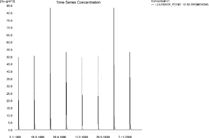
Figure 3.41. Concentrations of spring-applied bromoxynil in sandy loam pond.
Figur 3.41. Koncentration af forårsudbragt bromoxynil i morænelersvandhullet.

Figure 3.42. Concentrations of autumn- applied bromoxynil in sandy loam pond.
Figur 3.42. Koncentration af autumn-applied bromoxynil i morænelersvandhullet.
Figure 3.43 and Figure 3.44 show the concentration of bromoxynil on macrophytes in the pond. The concentrations are significantly lower than the concentrations in the water phase. Porewater concentrations are shown in Figure 3.45 and Figure 3.46. They are quite small, and the concentration adsorbed to sediment is 0.17 ng/kg for the spring application and <0.01 ng/kg for the autumn application.
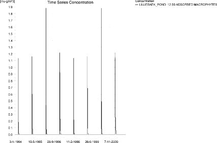
Figure 3.43. Spring-applied bromoxynil sorbed to the macrophytes in the sandy loam pond.
Figur 3.43. forårsudbragt bromoxynil sorberet til makrofytter i morænelers-vandhullet.
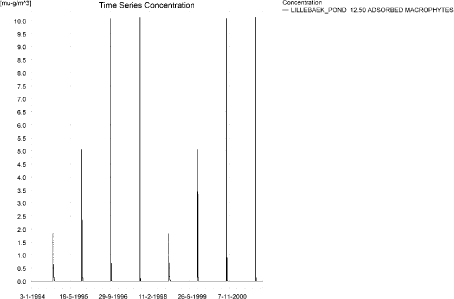
Figure 3.44. Autumn-applied bromoxynil sorbed to the macrophytes in the sandy loam pond.
Figur 3.44. Efterårsudbragt bromoxynil sorberet til makrofytter i morænelers-vandhullet.
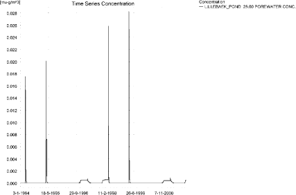
Figure 3.45. Pore water concentration following spring-application of bromoxynil in the sandy loam pond.
Figur 3.45. Porevandskoncentration efter forårsudbragt bromoxynil i morænelersvandhullet.
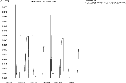
Figure 3.46. Pore water concentration following autumn-application of bromoxynil in the sandy loam pond.
Figur 3.46. Porevandskoncentration efter efterårsårsudbragt bromoxynil i morænelersvandhullet.
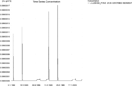
Figure 3.47. Concentration of bromoxynil in sediment following spring-application in the sandy loam pond. Note that the unit is µg/g sediment and not µg/m³ as indicated.
Figur 3.47. Koncentration af bromoxynil i sediment efter forårsudbringning i morænelersvandhullet. Koncentrationen er i µg/g sediment og ikke µg/m³ som angivet.
In Table 3.17, global maxima and time weighted concentrations (up to 7 days) are extracted.
Table 3.17. Actual and time weighted concentrations of bromoxynil, ng/l, in the sandy loam pond.
Tabel 3.17. Beregnede og tidsvægtede koncentrationer (ng/l) af bromoxynil i morænelersvandhullet.
| Spring application | Autumn application | |||||||
| Year | Bromoxynil | Actual | Time-weighted | Date | actual | Time-weighted | Date | |
| 1994 | global max | 50 | 02-04-1994 | 80 | 07-10-1994 | |||
| 1 hour(after max) | 47 | 48 | 76 | 78 | ||||
| 1 day after sp.in. | 30 | 37 | 54 | 62 | ||||
| 3 days | 16 | 27 | 36 | 50 | ||||
| 4 days | 11 | 24 | 30 | 46 | ||||
| 7 days | 4 | 16 | 17 | 36 | ||||
| 1995 | Global max | 51 | 01-04-1995 | 228 | 07-10-1995 | |||
| 1 hour | 48 | 50 | 198 | 211 | ||||
| 1 day | 33 | 39 | 89 | 124 | ||||
| 2 days | 19 | 30 | 40 | 82 | ||||
| 4 days | 14 | 26 | 26 | 69 | ||||
| 7 days | 6 | 19 | 8 | 46 | ||||
| 1996 | global max | 83 | 01-04-1996 | 469 | 07-10-1996 | |||
| 1 hour | 77 | 80 | 348 | 396 | ||||
| 1 day | 46 | 58 | 100 | 166 | ||||
| 2 (3*)days | 27 | 43 | 33 | 95 | ||||
| 4 days | 20 | 38 | 19 | 78 | ||||
| 7 (6*)days | 9 | 28 | 4 | 48 | ||||
| 1997 | global max | 53 | 01-04-1997 | 471 | 07-10-1997 | |||
| 1 hour | 51 | 52 | 349 | 397 | ||||
| 1 day | 36 | 42 | 100 | 166 | ||||
| 2 (3*)days | 25 | 34 | 33 | 95 | ||||
| 4 days | 20 | 31 | 19 | 78 | ||||
| 7 (6*)days | 11 | 24 | 4 | 48 | ||||
| 1998 | global max | 50 | 01-04-1998 | 80 | 06-10-1998 | |||
| 1 hour | 47 | 48 | 76 | 78 | ||||
| 1 day | 30 | 37 | 54 | 62 | ||||
| 2 (3*)days | 16 | 27 | 36 | 50 | ||||
| 4 days | 11 | 24 | 30 | 46 | ||||
| 7 (6*)days | 4 | 16 | 17 | 36 | ||||
| 1999 | global max | 51 | 31-03-1999 | 228 | 06-10-1999 | |||
| 1 hour | 48 | 50 | 198 | 211 | ||||
| 1 day | 33 | 39 | 89 | 124 | ||||
| 2 (3*)days | 19 | 30 | 40 | 82 | ||||
| 4 days | 14 | 26 | 26 | 69 | ||||
| 7 (6*)days | 6 | 19 | 8 | 46 | ||||
| 2000 | global max | 83 | 31-03-2000 | 469 | 06-10-2000 | |||
| 1 hour | 77 | 80 | 348 | 396 | ||||
| 1 day | 46 | 58 | 100 | 166 | ||||
| 2 (3*)days | 27 | 43 | 33 | 95 | ||||
| 4 days | 20 | 38 | 19 | 78 | ||||
| 7 (6*)days | 9 | 28 | 4 | 48 | ||||
| 2001 | global max | 53 | 31-03-2001 | 471 | 06-10-2001 | |||
| 1 hour | 51 | 52 | 349 | 397 | ||||
| 1 day | 36 | 42 | 100 | 166 | ||||
| 2 (3*)days | 25 | 34 | 33 | 95 | ||||
| 4 days | 20 | 31 | 19 | 78 | ||||
| 7 (6*)days | 11 | 24 | 4 | 48 | ||||
| max values | ||||||||
| global max | 83 | 471 | ||||||
| 1 hour | 77 | 80 | 349 | 397 | ||||
| 1 day | 46 | 58 | 100 | 166 | ||||
| 2 days | 27 | 43 | 40 | 95 | ||||
| 4 days | 20 | 38 | 30 | 78 | ||||
| 7 days | 11 | 28 | 17 | 48 | ||||
Figure 3.48, Figure 3.49, Table 3.18 and Table 3.19 show the output from the PestSurf template with time series identical toFigure 3.41 an Figure 3.42.
The concentrations of the FOCUS SW-scenario D4, pond are 26 ng/l for the spring application and 39 ng/l for the autumn application. PestSurf reaches 83 and 471 ng/l for the spring and autumn application, respectively. The highest concentrations are reached during dry periods, with relatively low water levels. A systematic difference between the D4-pond and the PestSurf pond is the size, The sandy loam pond is 250m² while the D4 pond is 900 m². It is therefore expected that the concentration level in the PestSurf sandy loam pond should be higher than for the D4 pond, when the major source is wind drift.
The concentrations in the sediment were 49 and 65 ng/kg for the FOCUS-D4-pond-scenarios, while they were 0.17 and below 0.01 ng/kg for the PestSurf simulations. The low concentrations in the pond and the fast disappearance does not allow time for much diffusion to the porewater and sorption to the sediment.
Click here to see Figure 3.48.
Figure 3.48. Overview for spring applied bromoxynil in the sandy loam pond generated by the PestSurf excel template. The time series shown is identical to the one in Figure 3.41. The detection value was set to 1 ng/l.
Figur 3.48. Oversigt for forårsudbragt bromoxynil i morænelersoplandet genereret med PestSurf-excel-skabelonen. Den viste tidsserie er mage til den i Figur 3.41. Detektionsgrænsen er sat til 1 ng/l.
Click here to see Figure 3.49.
Figure 3.49. Overview for autumn-applied bromoxynil in the sandy loam pond generated by the PestSurf excel template. The time series shown is identical to the one in Figure 3.42. The detection value was set to 1 ng/l.
Figur 3.49. Oversigt for efterårsudbragt bromoxynil i morænelersoplandet genereret med PestSurf-excel-skabelonen. Den viste tidsserie er mage til den i Figur 3.42. Detektionsgrænsen er sat til 1 ng/l.
Table 3.18. Part of the result sheet generated by the PestSurf Excel sheet for spring application of bromoxynil. The limiting values applied in the table is lowest detection valuε = 1 ng/l, toxicity to fish, daphnies and algae are set to 10, 100 and 1000 ng/, respectively. The recorded peaks are shown in Figure 3.48.
Tabel 3.18. Uddrag af resultatpresentationen genereret af PestSurf-Excel-arket for forårsudbragt bromoxynil. Grænseværdien anvendt i tabellen er detektionsgrænsen, 1 ng/l mens toxicitetsværdierne for fisk, dafnier og alger er henholdsvis 10, 100 og 1000 ng/l. De tabellerede hændelser er vist i Figur 3.48.
Table 3.19. Part of the result sheet generated by the PestSurf Excel sheet for autumn- applied bromoxynil. The limiting values applied in the simulation is lowest detection valuε = 1 ng/l, toxicity to fish, daphnies and algae are set to 10, 100 and 1000 ng/, respectively. The recorded peaks are shown in Figure 3.49.
Tabel 3.19. Uddrag af resultatpresentationen genereret af PestSurf-Excel-arket for efterårsudbragt bromoxynil. Grænseværdien anvendt i tabellen er detektionsgrænsen, 1 ng/l mens toxicitetsværdierne for fisk, dafnier og alger er henholdsvis 10, 100 og 1000 ng/l. De tabellerede hændelser er vist i Figur 3.49.
Table 3.20. Summary of simulation results for bromoxynil.
Tabel 3.20. Opsummerede resultater for bromoxynil.
3.5 Summary of Simulations
The maximum actual concentrations for all simulations are recorded in Table 3.20.
The concentration generated by PestSurf for the sandy pond is about 40 % of the concentration generated by FOCUS SW D3-ditch, while the concentration in the sandy stream is 3-4 times higher. The reason for the high concentrations in the stream is the simultaneous spraying of the total agricultural area. The maximum concentration level is reached 1111 and 1049 m from the upstream point, for the spring and autumn-applications, respectively. 112 m from the upstream end, the concentrations are 83 and 234 ng/l for the spring and autumn-application. These concentrations are considerably lower than the concentrations found in the D3-ditch (759 and 1143 ng/l). However, the concentrations cannot be compared directly because the top end of the PestSurf sandy catchment is protected by 20 m bufferzone. The water depth at the time of spraying is 14 and 9.5 cm for the spring and autumn-application time respectively, 112 m from the upstream end.
For the sandy loam pond, PestSurf generates a concentration that is about three times as high for the spring application and 12 times as high for the autumn application. For this particular autumn application, the water depth is only 21 cm (a factor 5), while the water depth for the spring application is 76 cm (a factor 1.3). A basic difference between the FOCUS D4-pond and the PestSurf sandy loam pond is the size, 900 m² against 250 m², which means that the PestSurf sandy loam pond is more exposed to wind drift. A rough estimate of the difference in exposure is a factor 2.4.
For the sandy loam stream, the PestSurf-concentrations are 10 and 18 times higher than the concentrations generated by FOCUS SW, for the spring and autumn applications, respectively. As for the sandy stream, this is due to the simultaneous spraying of the whole agricultural area and very limited water depth at the time of spraying, particularly for the autumn application during a dry autumn, where the water depth varied between 3 and 9 cm over the stream. The maximum value is reached near the end of the catchment. 125 m from the upstream end, the maximum concentration is 3990 and 7188 ng/l, with a corresponding water depth of 4.8 and 3.5 cm. Taking the difference in water concentration into account, the concentration levels correspond quite well. The maximum concentration on the stretch, where the stream is permanent and upstream of the groundwater influence is 3.13 µg/l and 7.74 µg/l, 625 m from the upstream end.
All maximum concentrations are generated by drift in both models Macrophyte concentration do not have a significant influence on the concentrations in the water phase in any of the scenarios, since bromoxynil has a low logKow. The sediment concentrations are very low in PestSurf for all scenarios, and considerably lower than the ones calculated in the FOCUS SW-scenarios. The concentrations correspond to the concentrations in the porewater, which are governed by the diffusion coefficient, and therefore also by the duration of high concentrations in the water phase.
Version 1.0 December 2006, © Danish Environmental Protection Agency