Systems Analysis of Organic Waste Management in Denmark2 The ORWARE model2.1 The conceptual model2.2 The core system 2.2.1 Organic household waste 2.2.2 Collection and transportation of waste 2.2.3 Incineration 2.2.4 Central composting 2.2.5 Anaerobic Digestion 2.2.6 Landfilling of waste 2.2.7 Gas engine 2.2.8 Spreading of organic fertilisers and nitrogen turnover in soil 2.3 The compensatory system 2.3.1 District heating 2.3.2 Electrical power 2.3.3 Mineral fertiliser ORWARE is a tool for environmental systems analysis of waste management. It is a computer-based model for calculation of substance flows, environmental impacts, and costs of waste management. According to Nybrant et al (1995), ORWARE was initially intended as a systems analysis tool for assessment of environmental impact from biodegradable waste handling in municipal waste management systems. The aim was to enable quantified and systematic comparison of the environmental impacts of different means to handle biodegradable waste, both solid and liquid waste. Modelling waste flows in total amounts and as specific substances and its related energy turnover did this. ORWARE has since then been expanded to cover handling of inorganic fractions in municipal waste as well. The ORWARE model has been developed in close co-operation between four different research institutions in Sweden: KTH - Royal Institute of Technology, IVL - Swedish Environmental Research Institute, JTI - Swedish Institute of Agricultural and Environmental Engineering and SLU - Swedish University for Agricultural Sciences. ORWARE consists of a number of separate submodels, which may be combined to design a waste management system for e.g. a city, a municipality or a company (Dalemo et al, 1997). ORWARE is a model primarily for material flows analysis (MFA). The material flows from different sources (wastes) through different methods for waste treatment (composting, anaerobic digestion etc) to different end uses (spreading of residues on agricultural soil or landfill). Emissions from transports, treatments etc are allocated as emissions to air, water and soil. Using methodology for impact analysis from life cycle assessment (LCA) different environmental impact categories is calculated (ISO 14042:2000).
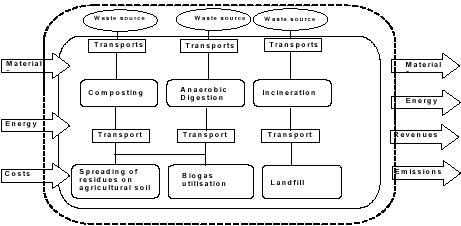
2.1 The conceptual modelThe ORWARE model consists of a core system, up- and downstream systems and a compensatory system (Eriksson et al, 2002). The core system describes the waste management system, including collection, treatment, and final disposal of waste generated within a defined geographical area and time-space. Up- and downstream processes are defined as those processes that impact the core system when using materials and energy. For example, production and distribution of diesel fuel used for collection and transportation is defined as upstream processes. Upstream processes also include waste sources and electricity and fuel generation and downstream processes are as example use of organic fertiliser and biogas utilisation (Figure 1). Figure 1. Conceptual model describing the waste management system in the ORWARE model as adapted to Denmark. From the core system functions or utilities are identified, for example distance travelled by car or bus using biogas or hydrogen as fuel, processed raw materials, organic fertilisers spread to crops, electricity generation etc. The scenarios contribute different amounts of each defined function and the compensatory system supplies the need of a certain function, so that all scenarios use the same amount of functions and thereby are comparable with each other. All submodels in ORWARE calculate the emissions and use of resources from the specific material treated. Therefore, the submodels do not need an optimal mixture of materials to function properly, but calculates the contribution from each specific material they treat.
2.2 The core systemThe core system is the physical system studied. In this study the core system describes handling of organic household waste from collection at household level to end use, for example landfilling of ash and slag from incineration and spreading of organic fertilisers. 2.2.1 Organic household wasteHousehold waste consists of different waste fractions, where organic household waste is one of them. The organic fraction of the total household waste is as an average 30 % – 40 % of the total amount of household waste (Sonesson and Jönsson 1996). In Tabel 1 is the most important parameters describing organic household waste are listed. For the full description of the organic waste, see Appendix E. The dry matter content for organic household waste used in the ORWARE model is assumed, as an average, to be 30 % (Jepsen, 2002). Tabel Key parameters in the ORWARE vector describing organic household waste in kg per kg dry matter (Sonesson and Jönsson 1996 and Sundqvist et al, 1999).
1 The sum of the different carbon fractions is TOC 2.2.2 Collection and transportation of wasteThere are different types of submodels describing vehicles for different types of transports. For collection of waste, there are back-packer and front-loader models. For transport of primary and secondary waste like fly ash and slag there are three submodels: ordinary truck, truck and trailer and barge for transports at sea. Data on average load, average speed etc. is used as input in all transport submodels. The output is total energy consumption, time consumption and costs. Emissions are calculated from the energy consumption. The transport submodel is further described in Sonesson (1996) and in Sonesson (1998). For more information about transports used in this project, see Appendix D. 2.2.3 IncinerationThe incineration submodel consists of three parts: pre-treatment, incinerator and air pollution control. The pre-treatment provides baling of the incoming waste, which makes it possible to store waste and to combust it later. In the incinerator, the waste is combusted and the outputs are raw gas, slag and fly ash. The raw gas is led to the air pollution control and the clean gas is released as air emissions. A submodel for flue gas condensing is included which may be used for more efficient energy recovery. Condense water is cleaned before it is emitted. Ash and slag are transported to landfill. The energy recovered in this submodel is district heating and/or electricity. As for all submodels, site-specific data are used as much as possible. When such data are missing, the attempt has been to use data from 1) comparable facilities, 2) other waste incinerators, or 3) reasonable assumptions. Emission factors are calculated from material balances from each process and are either product related (linearly dependant on the incinerated amount of the substance), process related (dependant on the amount of waste incinerated) or threshold related. The last category is modelled to generate a constant emission level depending on some threshold value, defined as the legislative threshold values are always kept. This approach is realistic for emissions that are normally adjusted within very narrow limits, e.g. NOx. The reason is usually economic; threshold values must be kept, but further reductions would not be economically motivated. A more detailed description of the waste incineration plant is found in Björklund (1998). Information about waste incineration plant used in this project, see Appendix D. 2.2.4 Central compostingIn ORWARE, three different types of composting are modelled (Sonesson, 1996). The different types are home composting, windrow composting and reactor composting. The models are based on the assumption that the composts are well managed, i.e. no failures occur that will give rise to high emissions of methane and other products of anaerobic conditions. All leachate water is returned to the compost. The degradation process is the same for all three compost types except for the degradation speed. The emissions are theoretically the same. The different compost submodels generate the same composition of the compost product when processing the same type of waste. When it comes to energy consumption the reactor compost demands most electricity, whereas composting in private households does not need energy at all (just some physical power that is not accounted for). Windrow composting is slightly less energy consuming than the reactor compost. The large scale composting has an option to clean the compost gas from ammonia (NH3) and nitrogen oxides (NOx). The cleaning equipment consists of a condensation step with recycling of condense liquid to the compost process and a bio-filter consisting of mature compost. The nitrogen captured in the filter is returned to the mature compost. The reactor compost submodel also gives a possibility to recover some of the heat released during the degradation. For more information about the compost submodel, see Sonesson 1998. Data and assumptions for this project are described in Appendix D. 2.2.5 Anaerobic DigestionThe submodel for anaerobic digestion is suitable for a mesophilic (37 ºC) or thermophilic (55 ºC) process (Dalemo, 1996). The model is based on a real treatment plant in Uppsala, which is a continuous single stage mixed tank reactor (CSTR). The incoming material is cleared from plastic bags and metals and then fragmentised. The separation will result in a loss of organic material. After hygienisation at 70 oC or 130 oC, the substrate is brought to the digester. The model automatically calculates the energy needed for hygienisation and digestion as well as need of water for adjustment of the dry matter content (DM). After the digestion step, the substrate passes through a heat exchanger and dewatering equipment. The amount of gas generated is dependent on the composition of different organic compounds as fat (C-fat), protein (C-prot), cellulose (C-chmd), hemicellulose and lignine (C-chsd), rapidly degradable carbohydrates (C-chfd) and the hydraulic retention time (HRT). The sludge from the digester is either separated into a solid and a liquid phase in the dewatering process or utilised without dewatering. The digestion residue (anaerobic sludge) is stored in large covered lagoons in solid or liquid phase. Liquid from dewatering is either recycled back to reactor or processed elsewhere, for instance pumped to sewage plant, reed bed etc. Electricity is consumed for mixing, pumping and drying. The submodel delivers anaerobic sludge, dried or wet, for spreading and biogas to be combusted. Further description can be found in Dalemo (1999). Data for the model used in this project is described in Appendix D. 2.2.6 Landfilling of wasteThe landfill submodel is divided into five different landfill types: mixed waste, bio-cell, sludge, fly ash and slag. The submodels are thought to work as Swedish average landfills, and the site-specific adjustments are few. There is a possibility to adjust the efficiency of the landfill gas recovery as well as the type of leachate treatment used. Energy consumption in form of electricity and diesel oil is accounted for and product outcome is bio-cell. Energy is generated as heat and or electricity from gas-fired engines, see the description of gas utilisation. Waste landfilled today will cause emissions during a long period of time. A dilemma is how to compare the emissions from the landfill with the instant emissions from the other processes in the system. Just to include instant landfill emissions would be to heavily underestimate the total impact. However, if one tries to estimate the total emissions the uncertainty will be large and the time perspective will not be comparable to other processes. As a compromise the future impact from landfilling has been separated in two time-periods, the definitions of which are a bit different between the different landfill types:
Leachate formed in the landfill is collected and treated before emitted to recipient. The landfill submodel uses biological treatment of leachate with chemical precipitation of phosphorus. During surveyable time, 80 % of phosphorus in leachate is precipitated and recycled back to the landfill. The rest of the phosphorus is emitted into recipient. Of nitrogen in leachate, 90 % is emitted as nitrogen gas (N2) to air, and the rest of the nitrogen is emitted to recipient. The landfill submodel (bio-cell not included) is further described in Björklund (1998), appendix D and the bio-cell in Fliedner (1999). Specific assumptions for this project are described in Appendix D. 2.2.7 Gas engineBiogas from the digester and landfill gas, which is partly collected, is combusted in a stationary gas engine. The energy generated during combustion is utilised as heat and electricity. Landfill gas formed but not collected is partly oxidised into landfill cover the rest is emitted to air mainly as methane (CH4) and carbon dioxide (CO2). 2.2.8 Spreading of organic fertilisers and nitrogen turnover in soilThe submodel for spreading of organic fertiliser is divided into three steps:
An ordinary truck performs transportation of residues; see description for the transport submodels above. The distance to and the area of each spreading area are used as input data and the model calculates the total distance and energy consumption. Two different spreaders are modelled, one for liquid products and one for solid products. The model determines what kind of spreader is needed depending on the dry matter content. The spreading model calculates the emissions from the truck transport and the spreading procedure and energy consumption for the vehicles. Nitrogen turnover is a down-stream process in the waste treatment flow in ORWARE. It is used as a complement to the organic fertiliser-spreading submodel. Nitrogen in organic fertiliser is assumed to be utilised by plants, organically bound to microorganisms etc. in soil (Dalemo et. al., 1998). The model calculates the emissions of nitrogen compared to use of mineral fertiliser. Thus, relative rather than absolute values are calculated as in the other submodels. Nitrogen is assumed to exist in three forms: ammonium (NH4), nitrate (NO3) and organically bound (N-org). The model gives emissions from mineralization of organically bound nitrogen during the first year after spreading and the long-term effects of mineralization. The efficiency with which the crops use the organic fertilisers compared to the mineral fertilisers are 100 % for phosphorus, 80 % of the mineral nitrogen and 30 % of the organically bound nitrogen. The emissions of nitrous oxide (N2O), NO3 and ammonia (NH3) depend on the soil condition, spreading conditions and climatic region can be adjusted in the model. The arable land submodel is further described in Dalemo et al (1998). The sub-models for spreading and nitrogen turnover in soil are further described in Sundqvist et al (2000) and Appendix D. 2.3 The compensatory systemIn order to fulfil the need of function (utilities) generated from management of waste in the core system. ORWARE supplements the lack of a function from an external source, that all scenarios have the same amount of functions, but from different sources. 2.3.1 District heatingGeneration of district heating can be included both as an up-stream process to waste management when needed in a waste treatment process, or as a compensatory process if necessary to fulfil a functional unit. Conventional district heating can be generated from biomass, oil or coal. The emissions from coal combustion use the same data source as for electricity production from coal, but with another degree of efficiency, 88 %, compared to degree of efficiency for electrical power generation, se below. 2.3.2 Electrical powerLike district heating, electricity generation may be included as both an up-stream process to the waste management system and as a compensatory process. It is possible to use one single source or a combination, a power mix. The different power sources in the model are biomass, hydropower, wind power, nuclear power, natural gases, oil and coal. Data on Swedish facilities are used except for the coal plant where data is used which describes the emissions from an average coal condense power station in Denmark. The degree of efficiency for condense power is 44 %. 2.3.3 Mineral fertiliserCompensatory production of the mineral fertilisers’ nitrogen (N), phosphorus (P) and potassium (K) is done in order to fulfil the functional unit of nutrients spread on arable land. Emissions and use of resources are related to the actual nutrient (emission per kg N, P or K) and not the fertiliser containing the nutrient and thereby directly to the functional unit. The submodels for compensatory production of mineral fertiliser cover extraction and manufacturing of raw materials and production of nitrogen, phosphorus and potassium fertiliser. The compensatory production of mineral fertiliser includes use of resources and emissions when producing mineral fertilisers. Spreading of mineral fertilisers is not included into compensatory mineral fertilisers. A life cycle inventory by Davies and Haglund (1999) using western European average data for production of mineral fertilisers are used for estimation the contribution from mineral fertiliser production. Emissions from mineral fertiliser nitrogen is calculated from manufacturing ammonium nitrate (35 % N), Western European average data, phosphorus mineral fertiliser is calculated from Triple superphosphate, TSP (48 % P2O5), Western European average data and potassium from PK fertiliser (22 % P2O5, 22 % K2O) Western European average data. |