| Front page | | Contents | | Previous | | Next |
Systems Analysis of Organic Waste Management in Denmark
Appendix D
Table C3.
Distribution of Mercury (Hg) expressed as kg per year.
| Mercury, Hg |
Reference |
Biogas 2004 |
Biogas long term |
Compost 2004 |
Compost long term |
| Core system |
|
|
|
|
|
| Sources |
6 |
6 |
6 |
6 |
6 |
| Air |
0.18 |
0.17 |
0.14 |
0.17 |
0.12 |
| Soil |
0.3 |
1 |
2 |
1 |
2 |
| Water |
0.006 |
0.0059 |
0.0048 |
0.0058 |
0.0041 |
| Left in landfill |
5 |
5 |
4 |
5 |
3 |
| Left in material |
0 |
0.04 |
0.03 |
0.04 |
0.03 |
| External system |
|
|
|
|
|
| Air |
0.07 |
0.06 |
0.03 |
0.10 |
0.19 |
| Water |
0.37 |
0.33 |
0.26 |
0.74 |
1.79 |
| Soil |
0.00 |
0.00 |
0.00 |
0.00 |
0.00 |
| Left in landfill |
0.00 |
0.00 |
0.00 |
0.00 |
0.00 |
| Left in material |
0.00 |
0.00 |
0.00 |
0.00 |
0.00 |
| Sum external |
0.44 |
0.39 |
0.29 |
0.84 |
1.98 |
Table C4.
Distribution of copper (Cu) expressed as kg per year.
| Copper, Cu |
Reference |
Biogas 2004 |
Biogas long term |
Compost 2004 |
Compost long term |
| Core system |
|
|
|
|
|
| Sources |
7 160 |
7 158 |
7 154 |
7 158 |
7 153 |
| Air |
0.07 |
0.07 |
0.05 |
0.06 |
0.05 |
| Soil |
362 |
864 |
2071 |
1048 |
2782 |
| Water |
34 |
32 |
26 |
31 |
22 |
| Left in landfill |
1 612 |
1 493 |
1 205 |
1 449 |
1 037 |
| Left in material |
5 151 |
4 770 |
3 853 |
4 630 |
3 312 |
| External system |
|
|
|
|
|
| Air |
3 |
2 |
0.59 |
3 |
4 |
| Water |
82 |
73 |
58 |
164 |
410 |
| Soil |
0 |
0 |
0 |
0 |
0 |
| Left in landfill |
0 |
0 |
0 |
0 |
0 |
| Left in material |
0 |
0 |
0 |
0 |
0 |
| Sum external |
84 |
75 |
59 |
167 |
414 |
Table C5.
Distribution of Chrome (Cr) expressed as kg per year.
| Chrome, Cr |
Reference |
Biogas 2004 |
Biogas long term |
Compost 2004 |
Compost long term |
| Core system |
|
|
|
|
|
| Sources |
2 167 |
2 162 |
2 148 |
2 160 |
2 143 |
| Air |
1.1 |
1.0 |
0.8 |
1.0 |
0.7 |
| Soil |
106 |
254 |
609 |
308 |
818 |
| Water |
0.56 |
0.52 |
0.41 |
0.50 |
0.36 |
| Left in landfill |
847 |
784 |
632 |
761 |
544 |
| Left in material |
1 212 |
1 122 |
907 |
1 089 |
779 |
| External system |
|
|
|
|
|
| Air |
2 |
2 |
0.38 |
2 |
3 |
| Water |
60 |
54 |
43 |
121 |
302 |
| Soil |
0 |
0 |
0 |
0 |
0 |
| Left in landfill |
0 |
0 |
0 |
0 |
0 |
| Left in material |
0 |
0 |
0 |
0 |
0 |
| Sum external |
63 |
56 |
43 |
123 |
306 |
Table C6.
Distribution of Nickel (Ni) expressed as kg per year.
| Nickel, Ni |
Reference |
Biogas 2004 |
Biogas long term |
Compost 2004 |
Compost long term |
| Core system |
|
|
|
|
|
| Sources |
1 497 |
1 495 |
1 490 |
1 494 |
1 487 |
| Air |
1.9 |
1.8 |
1.4 |
1.7 |
1.2 |
| Soil |
75 |
178 |
426 |
216 |
573 |
| Water |
1.1 |
1.0 |
0.8 |
1.0 |
0.7 |
| Left in landfill |
393 |
363 |
293 |
353 |
252 |
| Left in material |
1 027 |
951 |
768 |
923 |
660 |
| External system |
|
|
|
|
|
| Air |
187 |
148 |
54 |
135 |
4 |
| Water |
69 |
61 |
49 |
138 |
345 |
| Soil |
0 |
0 |
0 |
0 |
0 |
| Left in landfill |
0 |
0 |
0 |
0 |
0 |
| Left in material |
0 |
0 |
0 |
0 |
0 |
| Sum external |
256 |
209 |
103 |
273 |
349 |
Table C7.
Distribution of Zink (Zn) expressed as kg per year.
| Zink, Zn |
Reference |
Biogas 2004 |
Biogas long term |
Compost 2004 |
Compost long term |
| Core system |
|
|
|
|
|
| Sources |
16949 |
16937 |
16908 |
16934 |
16896 |
| Air |
0.5 |
0.4 |
0.4 |
0.4 |
0.3 |
| Soil |
852 |
2032 |
4872 |
2466 |
6546 |
| Water |
3 |
3 |
2 |
3 |
2 |
| Left in landfill |
9843 |
9113 |
7358 |
8846 |
6328 |
| Left in material |
6252 |
5789 |
4676 |
5619 |
4020 |
| External system |
|
|
|
|
|
| Air |
3 |
2 |
0.7 |
3 |
5 |
| Water |
101 |
90 |
72 |
202 |
506 |
| Soil |
0 |
0 |
0 |
0 |
0 |
| Left in landfill |
0 |
0 |
0 |
0 |
0 |
| Left in material |
0 |
0 |
0 |
0 |
0 |
| Sum external |
104 |
92 |
73 |
206 |
511 |
Table C8.
Distribution of dioxin expressed as kg per year.
| Dioxin |
Reference |
Biogas 2004 |
Biogas long term |
Compost 2004 |
Compost long term |
| Core system |
|
|
|
|
|
| Sources |
1.89E-05 |
1.89E-05 |
1.89E-05 |
1.89E-05 |
1.89E-05 |
| Air |
6.65E-05 |
6.11E-05 |
4.80E-05 |
5.97E-05 |
4.26E-05 |
| Soil |
9.58E-07 |
2.29E-06 |
5.48E-06 |
2.77E-06 |
7.36E-06 |
| Water |
2.66E-05 |
2.44E-05 |
1.92E-05 |
2.39E-05 |
1.71E-05 |
| Left in landfill |
3.38E-02 |
3.11E-02 |
2.44E-02 |
3.03E-02 |
2.17E-02 |
| Left in material |
2.66E-03 |
2.44E-03 |
1.92E-03 |
2.39E-03 |
1.71E-03 |
| External system |
|
|
|
|
|
| Air |
1.42E-06 |
1.07E-06 |
1.60E-08 |
1.06E-06 |
1.97E-07 |
| Water |
0 |
0 |
0 |
0 |
0 |
| Soil |
0 |
0 |
0 |
0 |
0 |
| Left in landfill |
0 |
0 |
0 |
0 |
0 |
| Left in material |
0 |
0 |
0 |
0 |
0 |
| Sum external |
1.42E-06 |
1.07E-06 |
1.60E-08 |
1.06E-06 |
1.97E-07 |
ORWARE submodels
Collection and Transports
Models for trucks with and without trailer are used for calculating energy consumption, emissions and cost for transport of materials from one place to another. The difference between these trucks and the collection trucks is that loading and unloading is assumed an insignificant part of the transport and is therefore left out of the model. Otherwise, sub-models are identical in their structure differing only in the input data concerning fuel consumption, loading capacity etc. The model structure is shown in Figure D1
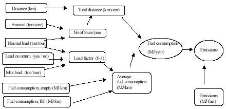
Figure D1. Model structure for transport models.
The number of loads required per year in the transport model is calculated from the amount of material to be transported and the normal load capacity for the specific type of material. The number of loads together with the distance between source and destination gives total drive distance per year. This total drive distance in turn is used for two purposes:
- To calculate total fuel consumption using average fuel consumption per km
- By using average speed, the total drive time per year is obtained which in turn gives the number of trucks required paving the ground for fixed cost calculation. The total drive time is also used for calculation of variable costs (e.g. salary etc.) that are functions of time consumed for transport.
Normal load and max load together with information about whether the truck is loaded on return or not gives basis for load factor i.e. what part of the max load is the actual average load. This load factor and data about fuel consumption both during max load and empty load gives average full consumption. The total fuel consumption is used together with emissions per MJ of fuel consumed to calculate emissions per year.
The structure of model provides it flexibility in different ways. Materials with lower density result in more number of loads with low average fuel consumption. It is simple to change many parameters so that changes in prices etc can be made. The biggest drawback lies in the assumption of the average speed, which regulates the drive time and in turn much of the cost calculations. Average speed should reflect the speed during the transport of the material during one year, including loading, unloading and the working days spent for maintenance etc. These parameters are difficult to estimate. Therefore, currently the average speed is calculated by dividing normal drive distances per year for long distances by the number of working hours per year. Table D1 shows input data in transport models, Table D2 shows emission data per MJ.
Table D1.
Input data for transport models.
| Input data |
Value |
| Max load, truck |
12 ton |
| Max load, truck and trailer |
35 ton |
| Average speed |
30 km/h 1 |
| Fuel consumption truck, empty |
2 litre / 10 km |
| Fuel consumption truck, full load |
3.5 litre / 10 km |
| Fuel consumption trailer, empty |
3 litre / 10 km |
| Tyre wear |
0.027 g tyre / MJ consumed fuel |
| Fuel consumption truck and trailer, full load |
5 litre / 10 km |
1Corresponding to a use of a truck for 1 760 hours per year and an annual drive distance of about 500 km.
Table D2.
Air emissions from trucks.
| Emission |
g/MJ |
| CO2 – fossil |
74 |
| CH4 |
0.001 |
| VOC |
0.066 |
| PAH |
0.0000025 |
| CO |
0.00029 |
| NOx |
0.53 |
| N2O |
0.0026 |
| SOx |
0.093 |
| Particles |
0.013 |
Input data for collection and transports sub-model in current study
The organic waste in Denmark is supposed to be collected and transported to incineration plant. At the incineration plant waste is sorted out to incineration, composting or to anaerobic digestion. Load and distances driven during collection and transportation of waste are shown in Table D3.
Input data parameters for collection:
- Fuel consumption: 0.3 GJ/ton waste (Hyldebrandt-Larsen, 2002)
- Energy content in diesel oil: 35.6 MJ/l diesel, (Hyldebrandt-Larsen, 2002)
Table D3.
Loads and distances for transports.
| Type of load |
From |
To |
Load1 [tonnes] |
Distance [km] |
| Waste (40 %) |
Incineration |
Anaerobic Digestion |
20 (35) |
80 |
| Waste (60 %) |
Incineration |
Anaerobic Digestion |
8 (12) |
20 |
| Waste |
Incineration |
Composting |
8 (12) |
10 |
| Reject |
Anaerobic Digestion |
Landfill |
10 (35) |
40 |
| Reject |
Composting |
Landfill |
25 (35) |
40 |
| Ash |
Incineration |
Landfill |
25 (35) |
40 |
| Slag |
Incineration |
Landfill |
10 (35) |
40 |
| Sludge |
Anaerobic Digestion |
Arable land |
10 (35) |
5 |
| Compost |
Composting |
Arable land |
25 (35) |
15 |
1 Normal load (Max load)
All vehicles are assumed empty during return transport, therefore when calculating emissions the actual distances are twice that are shown in Table D3. Using information from Table D4 the actual fuel consumption for collection and transportation can be calculated.
Table D4.
Fuel consumption for different trucks.
| Truck data |
Value |
Unit |
| Ordinary truck |
|
|
| Maximum load |
12 |
ton |
| Average speed |
30 |
km/ h |
| Fuel consumption, fully loaded |
35 |
l/ 100 km |
| Fuel consumption, empty |
20 |
l/ 100 km |
| Truck and trailer |
|
|
| Maximum load |
35 |
ton |
| Average speed |
30 |
km /h |
| Fuel consumption, fully loaded |
35 |
l/ 100 km |
| Fuel consumption, empty |
30 |
l/ 100 km |
Incineration
The data used for calculations is from 1996. Currently there are two varieties of the model, one describing the incinerator in Uppsala operated by Vattenfall and the second model for Fortums (former Birka Energy’s) incinerator at Högdalen in Stockholm. The model for Stockholm has been modified and further developed compared to the one described in Björklund (1998), appendix F. The changes made are shown in a recent project report to the Swedish Energy Administration (Sundqvist et al., 2002). In both cases, the models are site specific and use emission and data for mass flows measured at these facilities. The model is built up of three parts: pre-treatment, incineration chamber and flue gas cleaning. Figure D2 gives a schematic diagram of the structure valid for both models.
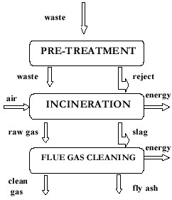
Figure D2.
Structure of the incineration model.
Pre-treatment
In pre-treatment, some parts of the incoming waste are separated for compression, wrapping and enclosing in a plastic. This possibility of wrapping can be utilised at times when the amount of incoming waste is much more than the capacity of the incinerator. This situation is often in the summer time where parts of the incineration facility are closed for maintenance. To avoid landfilling of combustible waste from the same municipality or waste from another municipality for landfilling somewhere else, the wrapping alternative is preferred. In terms of modelling this would mean 2 kg of plastic per ton of waste and electricity consumption of 14.5 MJ/ton waste. This data for wrapping is obtained from Åberg (1998).
Incineration
In the incineration chamber mixed waste is incinerated where an impure flue gas or raw gas is built up. Non-combustible part is separated in the form of slag. The raw gas is then taken to flue-gas cleaning facility where gas cleaning is performed with calculation of associated energy recovery, see figure A2. As part of the raw gas cleaning, condensation equipment and a water treatment facility to treat the condensed water are included. The gas cleaning part gives one stream of fly ash and another stream of clean gas.
Flue gas cleaning
Separation of pollutants and partitioning of substances is carried out in the model to the largest extent using a material balance. This is related to either the amount of a specific incoming substance or the total amount of incoming waste. It is logical to relate certain emissions to the prevailing permissible values e.g. for NOX, which is linearly dependent on the energy content of the waste. A material balance is not applied for such substances in the model.
During incineration in both sub-models, different components are partitioned as follows:
- How much of the heavy metals in the incoming waste ending up in the slag and raw gas are calculated first. Then calculation is done on how much of the metals in the raw gas go to the fly ash, sludge and wastewater and emissions to air. The fly ash and sludge are mixed together to give a stabilised cement-like material. Emissions to water and air are proportional to the amount of metals in the waste. Emissions to air for all heavy metals except mercury are less than 0.5 % of incoming amount. The ash and sludge resulting from the flue gas cleaning part and the slag from the incineration chamber are transported to a waste landfill site.
- Nitrogen oxide (NOx) and nitrous oxide (N2O) emission are calculated based in energy content. This depends on the fact that permissible amount of NOx emissions is given in units of kg NOx/ MJ.
- Calculations of sulphur oxides (SOx) are done in the same way as for nitrogen oxides.
- Dioxin emission is calculated from the amount of waste incinerated.
- Heat production in the model is calculated as heat from the energy content of the waste based on its composition. The energy recovery is calculated using the effective heating value and the moisture content of the waste. In the flue gas condenser, about 70 % of the theoretically available heat of the steam are recovered.
- The number and amount of chemical additives varies based on the facility.
Input data to the incineration model in this study
The basis for the model is waste incineration facility at Högdalen in Stockholm with a latest performance data from the environmental report of the facility for the year 2000. Baling of waste is not included and there is no flue gas condensation. Rest products from the facility like ash and slag are landfilled. Of the slag generated, 80 % is recycled in road construction and 20 % is landfilled. In Table D5 the parameters of incineration are described.
Table D5.
Performance parameters for incineration process.
| Parameter |
Value |
Unit |
| Total efficiency |
85 |
% of lower heat value |
| Electricity consumption |
0.32 |
MJ/kg waste |
| NOX - emission to air |
200 |
mg NO2/MJ waste |
| N2O - emission to air |
0.01 |
kg N-N2O/kg N in waste |
| NH3 - emission to air |
0.11 |
mg NH3/MJ waste |
| Dioxin formation |
0.2 |
ng dioxin/m3 flue gas |
| CO – emission |
3.29 |
mg CO/MJ waste |
| Particles/Dust |
0.50 |
mg particles /MJ waste |
| SO2-separation in flue gas cleaning |
95 |
% |
| HCl- separation in flue gas cleaning |
99.8 |
% |
| Alpha value for heat power operation |
0.35 |
MJ el/MJ heat |
Compost
In the ORWARE model three different types of composts is modelled:
- Large scale reactor compost with or without compost gas cleaning
- Large scale windrow compost with or without compost gas cleaning
- Small scale home composting
Microbial degradation processes occurring during composting are assumed same for the three compost techniques. Emissions during composting are theoretically the same for all types of composts. The model assumes that the composting process works under optimum conditions.
The compost model assumes that:
- The compost is well aerated during the whole process
- The compost is allowed to fully mature
- Dry matter content in matured compost is 50 %
- The time-factor is not regarded, only the processes from the beginning to the end of the compost process and not how long time it takes to decompose organic material
Organic matter is degraded during the compost process. Heat CO2, and some methane (CH4) are released and the mature compost consists of mainly humus-like substances. Different organic substances decompose to different degrees according to Table D6.
Table D6.
Degradation of organic compounds during composting (Sonesson, 1996).
| Substance |
% turned into CO2 |
% turned into humus |
| C-chsd (lignin) |
30 |
70 |
| C-chmd (cellulose) |
90 |
51 |
| C-chfd (starch, sugars) |
80 |
20 |
| C-fat |
60 |
40 |
| C-protein |
65 |
35 |
1After composting, there is a small residue of undegraded C-chmd. It is assumed that 5 % of incoming C-chmd is undegraded.
Depending on C/N-ratio in compost part of the nitrogen is volatilised as gas, primarily as NH3, but also as N2O and N2. The model calculates that of the total amount of nitrogen lost as gaseous emission 98 % is volatilised as NH3, 0,5 % as N2O and 1,5 % as N2 (Gunnarsdotter Beck-Friis, 2001).
Heavy metals are considered as inert material and the total amount fed into the compost equals the amount in matured compost. Because of degradation of organic compounds the concentration of metals on dry matter basis increases.
Input data to the compost model in this study
50 % of the waste to compost is put in windrow compost, 50 % in reactor compost. In both composts the carbon-nitrogen ratio has been set to 30, corresponding to an input of carbon-rich material. Differences between the two compost techniques are that the reactor compost has a higher use of electricity and diesel for running and maintenance of compost and that compost exhaust gases are cleaned in a bio-filter according to Table D7.
Generally a carbon-nitrogen of 30 is sufficient for reactor composting. In windrow composting is the carbon-nitrogen ratio probably higher than 30. Therefore are the nitrogen losses from windrow composting somewhat overestimated.
Table D7.
Performance parameters for the compost process.
| Type of compost |
Value |
Unit |
| Open windrow compost |
|
|
| Electricity consumption |
0 |
MJ/kg waste |
| Diesel consumption |
0.00151 |
MJ/kg waste |
| Compost gas cleaning |
No |
|
| Reduction of NH3 |
0 |
% |
| Reduction of N2O |
0 |
% |
| Reduction of CH4 |
0 |
% |
| Reactor compost |
|
|
| Electricity consumption |
0.1801 |
MJ/kg waste |
| Diesel consumption |
0.07551 |
MJ/kg waste |
| Compost gas cleaning |
Yes |
|
| Reduction of NH3 |
991 |
% |
| Reduction of N2O |
90 |
% |
| Reduction of CH4 |
50 |
% |
1 Valkainen (2002)
Anaerobic digestion
The original submodel for anaerobic digestion is described in Dalemo (1996). Incoming material to anaerobic digestion can be pre-treated by utilising bag- and metal separation, hygienisation at 70 °C or by sterilisation at 130 °C. During bag and metal separation parts of the material that clings to the bags are sorted out with the separated metal. If plastic bags are used the model assumes that 25 % of the waste clings to the plastic bags. When using paper bags the losses are only 1 % e.g. only losses from metal separation. Hygienisation is calculated as energy used for heating the material from ambient temperature to hygienisation or sterilisation temperature according to the formula: E = m * cp * T
The actual energy requirements are assumed to be 20 % higher than the calculated due to energy losses. Ambient temperature is assumed to be 10 °C as an yearly average temperature.
The anaerobic sub-model in ORWARE describes continuous single stage mixed tank reactor (CSTR) in steady state working under meso- or termophile conditions, 37 °C and 55 °C. After digestion the anaerobic sludge passes through a heat exchanger, where 50 % of the energy content (heat) is recovered. The exchanged heat is used for preheating the incoming material.
The anaerobic sludge can be dewatered, dried or not treated at all. Dewatered sludge has a dry matter content of 25 – 35 % and dried sludge 98 %. Dried sludge is turned into pellets and incinerated or as organic fertiliser, primarily phosphorus.
The anaerobic sludge is stored in covered storage for reducing ammonia (NH3) losses. Covered storage also gives the possibility to gather methane that is formed during storage.
The amount of biogas from anaerobic digestion depends of the incoming materials composition of organic carbon. The model is assuming degradation of organic Substances according to first order kinetics
D = D0/(1 + (1/k*HRT) where
D = Degradation ratio
D0 = Maximum degradation ratio
k = first order rate constant
HRT = Hydraulic retention time
Different organic substances are decomposed at different rates. To be able to calculate the degradation ratio for a mixture of waste substances, degradation is calculated from degradation of different organic compounds shown in table A 4.8.
Table D8.
Performance parameters for the anaerobic digestion process.
| Organic substances |
D0 |
K (days-1) |
% CH4 |
| C-chsd (lignin) |
0 |
0.001 |
50 |
| C-chmd (cellulose) |
1-1.77* C-chsd |
0.18 |
50 |
| C-chfd (starch. sugars) |
1.0 |
0.23 |
50 |
| C-fat |
0.8 |
0.13 |
69 |
| C-protein |
0.95 |
0.13 |
78 |
Energy for pumping and mixing of material etc. of different materials requires approximately 5 % of produced energy. Heat requirement in the digester is calculated from a mechanistic approach. Heat consumption depends on the temperature of the digested material and losses through the digester reactor during digestion. It is assumed that 50% of the heat in material leaving the digester can reused through a heat exchanger reducing the temperature from digester temperature to ambient temperature, thus reducing the need of heat.
Input data to the anaerobic digestion model in this study
- 50 % of the waste to anaerobic digestion is digested in a mesophilic process,
50 % in a thermofilic process.
- Biogas production is set to 125 nm3 per ton waste treated.
- Dry matter (DM) content in digestion chamber is set to 13 %. The incoming waste is therefore diluted using fresh water
- No recycling of anaerobic sludge to incoming waste
- 35 % of the incoming waste is sorted out to incineration.
- No dewatering of anaerobic sludge prior to spreading
- All anaerobic sludge is utilised as organic fertiliser
Landfilling of waste
Five different types of landfills are modelled; biocell (Fliedner, 1999), landfills for mixed waste, sludge, ash and slag (Björklund, 1998). The models are supposed to reflect Swedish average landfills and therefore site-specific modification of the models is limited.
Waste that is put into landfill today will continue to give out emissions for long time in the future. One dilemma is, thus, how to compare such emissions from landfills with more immediate emissions from other processes in the system. To include only the immediate emissions from landfills would be illogical representation of the total load. On the other hand to try to estimate the total emission brings about considerable magnitude of uncertainty and even so the time perspective becomes incomparable with the other processes. As a compromise, future impacts of landfills have been divided into two periods that have some differences for the different types of landfills (see Figure D3):
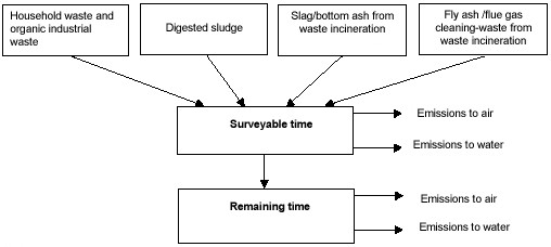
Figure D3. Material flow structure in the landfilling model.
Surveyable time (ST): During this time most of the reactive processes in landfills is subsided and the landfill apparently reaches a stationary condition. For mixed waste and sludge as well as bio-cell, the surveyable time is defined as the end of the methane generation phase. For slag and ash landfills the leakage of soluble salts defines the surveyable time. The surveyable time is consequently a functional measure of time and varies from case to case but generally it is in the order of 100 years.
Remaining, infinite time (RT): This time period covers until all the material in the landfill is spread out in the environment through the formation of gas, leakage, erosion and eventual inland icing. This infinite time embodies emissions in the worst scenario.
Calculations are based on the amount of waste to landfill during one year. The emission during the surveyable time is an average yearly emission under corresponding time from a landfill where the same amount of waste is put into landfill year after year. When emissions under this surveyable time are calculated, the emissions that will occur during the remaining time are also calculated. During assessment and discussions attention is paid only to those emissions under the surveyable time. In the sub-models for landfill of mixed waste and sludge, the following processes occur:
- Degradation of organic material gives emissions composed of mainly methane. Sugar, starch and fat are considered 100 % degradable, cellulose 70 % while lignin and plastic as non-degradable. The composition of the gas varies depending on composition of the organic material. In most of the cases, the gas contains 50 – 60 % CH4 and the rest mainly CO2.
- Leakage of heavy metals is small during the surveyable time, in the range 0.1 to 0.001 % of the amount to landfill.
- Nutrient leaks in the form of phosphorous (2 % of amount landfilled, 15 % for sludge) and nitrogen (90 % of the amount to landfill).
- For organic pollutants, there is lack of knowledge concerning their long-term fate in landfills. During the surveyable time, it is possible that such substances are formed, degraded, converted to gas, vaporised, leak out or adsorbed to the material in landfill. A very simplified estimate for every substance studied.
- The gas can be collected during the surveyable time with an efficiency of 50 % of the gas formed. The collected gas can be flared out or combusted in a gas motor. The remaining gas makes its way to the outer layer of the landfill where 15 % of the methane is oxidised to carbon dioxide.
The bio-cell model that handles only easy degradable organic waste is based on the landfill for mixed household waste. However, it gives considerably faster degradation (i.e. the surveyable time refers to a shorter time) and more effective gas collection than in conventional landfills (65 % of formed gas). Furthermore a leakage water of higher quality is formed. In this connection, a bio-cell is considered something between conventional landfill and digestion chamber. The main feature of ash and slag landfills is leakage of heavy metals. Metals in the ash leak out in the range of 1 to 10 % of the amount in during surveyable time. Metals in the slag have less tendency to leach out, the leakage correspond to 0,1 to 5 % of amount in landfill under the surveyable time. No gas is extracted from such landfills.
The leakage treatment model can be connected to all of the landfill submodels. The model reflects a biological treatment with a chemical precipitation. About 80 % of the phosphorus leaking out under the surveyable time are collected and recycled back to the landfill (it then leaks out during the remaining time). Furthermore 90% of the nitrogen leakage is partitioned as nitrogen gas with the rest going out with the leakage water. No metal partitioning is modelled. Working machines consume 40 MJ of diesel oil per ton material to landfill for all landfill sub-models. Table D9 depicts input data for landfill sub-model.
Table D9.
Parameters in landfill model during the surveyable time.
| Parameter |
Value |
Unit |
| degradation of sugar, starch, fat |
100 |
% of landfilled amount |
| degradation of cellulose |
70 |
% of landfilled amount |
| degradation of lignin and plastic |
0 |
% of landfilled amount |
| Leakage of phosphorus |
2 |
% of landfilled amount |
| Leakage of nitrogen |
90 |
% of landfilled amount |
| Leakage of heavy metals, MSW and sludge |
0.1 – 0.001 |
% of landfilled amount |
| Leakage of heavy metals, incineration ash |
1 - 10 |
% of landfilled amount |
| Leakage of heavy metals, incineration slag |
0.1 - 5 |
% of landfilled amount |
| treatment efficiency, N in leakage water |
90 |
% of leak water content |
| treatment efficiency, P in leakage water |
0.8 |
% of leak water content |
| Gas collection, mixed waste and sludge |
50 |
% of generated gas |
| Gas collection, biocell |
65 |
% of generated gas |
| Soil oxidation, methane |
15 |
% of methane leakage |
| Diesel consumption, all landfills |
40 |
MJ/ton landfilled material |
The gas (methane) recovered from landfills can be used as a fuel in a gas motor that can supply electricity and heat. The energy from gas motor is calculated using the energy content of the methane gas. If the gas is flared out, the emissions are calculated according to Table D11, with a zero energy recovery. When it is recovered, 30 % is electricity and 60 % heat but this also varies from case to case.
Input data to the landfill model in this study
In this study, when the industrial waste is landfilled, 50 % of the landfill gas produced is assumed collected (this is the same as for landfilling of organic waste). Around 90% of this collected gas is used for heat production in a gas motor. Treatment of leakage water (nitrogen and phosphorus) is supposed to be part of both types of landfilling (landfilling of industrial waste and landfilling of ashes and slag). Whenever results for landfilling are shown, they refer only to the emissions during the surveyable time.
Gas engine
Biogas formed during anaerobic digestion and from landfilling of organic waste can be used for different purposes. It can be used as:
- Vehicle fuel in cars and busses
- Combusted in a stationary gas engine for generation of electricity and heat
- Torched, only applied to landfill gas. The gas is combusted in a stationary gas engine, but no energy is recovered
Biogas as vehicle fuel
Before biogas can be utilised as vehicle fuel, it has to be upgraded to a higher fuel quality compared to the original biogas. Methane content is after upgrading 97 % and the amount of CO2 is less than 3 %. Up grading of biogas to vehicle fuel quality is done in two steps:
- Stripping of CO2
- Compression of cleaned biogas to 250 bars pressure
Both steps require an input of electricity amounting to 3 % of the energy produced.
Utilisation of biogas in a stationary gas engine for heat and power generation
Energy from combustion of biogas in a stationary gas-engine equals to the energy content of the produced biogas. If the energy is utilised as electricity and heat, 30 % of the energy in the biogas can be utilised as electricity and 60 % as heat. The remaining 10 % are assumed lost during combustion. Other emissions from a stationary gas engine are shown in Table D10.
Table D10.
Emissions from combustion of methane gas in a stationary gas motor (mg/MJ gas).
| Substance |
Emission [mg/ MJ gas] |
| CH4 |
100 |
| VOC |
160 |
| CO |
250 |
| NOx |
200 |
| Particles |
0 |
Input data to the anaerobic digestion model in this study
- All biogas is combusted in a stationary gas engine
- Energy is utilised as electricity and no heat is recovered. In this study 38 % of the energy in the biogas is utilised as electricity and 52 % as heat.
- Emissions factors for stationary gas engine are adapted to Danish data stating that Cleaning of sulphur emitted as sulphur dioxide is cleaned to 400 mg/m3 gas. New emission factors are shown in Table D11.
Table D11.
Emissions from incineration of methane gas from landfilling in a stationary gas motor (mg/MJ gas).
| Substance |
Emission |
| CH4 |
430 |
| VOC |
4 |
| CO |
250 |
| NOx |
100 |
| Particles |
0 |
Spreading of organic material on arable land and emissions from nitrogen turnover in the soil
The submodel for spreading of organic fertiliser and nitrogen turnover in soil has four different parts:
- Calculation of transportation from treatment plant to satellite storage in field
- Calculation of area needed to spread organic fertiliser
- Spreading of organic fertiliser
- Nitrogen turnover in soil
Calculation of transportation from treatment plant to satellite storage in field
Calculation of transport distances from treatment plant to arable land uses the acreage needed over longer time-period than one year. This acreage is different to the actual acreage available because more than one years yield is spread of organic fertiliser on each hectare. It is actually the average transport distance over a number of years that are calculated.
Calculation of area needed to spread organic fertiliser
Need of acreage for spreading of organic fertiliser is calculated for each fertiliser spread. The different organic fertilisers’ need of acreage is then added together to a total need of acreage. This total area needed is then used for calculating the
transport distances from storage to spreading. This calculates the total need of area inside a geographically defined area. In reality, is not the total acreage available because of different reasons. By multiplying the available area with a factor, that represents some kind of acceptance of spreading organic fertiliser, the total transport distance is calculated.
Spreading of organic fertiliser
Emissions from spreading of organic fertilisers are emissions from transport from storage on site to field and vehicle emissions during spreading. Ammonia volatilisation during spreading is also calculated.
Using dry or liquid spreader can do spreading. The model chooses appropriate spreader based on the organic fertiliser dry matter content. For dry matter content up to 10 % organic fertiliser are spread with liquid spreader. Dry spreader is used when dry matter content is above 10 %.
Table D12.
Data concerning dry and liquid spreaders.
| Spreader |
Value |
Unit |
| Dry spreader |
|
|
| Empty weight |
6 000 |
kg |
| Loading capacity |
3 750 |
kg |
| Speed during transportation to and from field |
15 |
km/hour |
| Speed during spreading |
5 |
km/hour |
| Liquid spreader |
|
|
| Empty weight |
4 000 |
kg |
| Tank volume |
8 000 |
l |
| Working width |
12 |
m |
| Speed during transportation to and from field |
15 |
km/ h |
| Speed during spreading |
4 |
km/ h |
For each organic fertiliser spread, the model calculates the distance from field storage to field and time and energy when spreading. Emissions per MJ fuel used for tractor pulling spreader are assumed same as for transportation. Ammonia volatilisation is a function of type of spreader, spreading technique etc. (Table D12).
Table D13.
Emissions of ammonia as a fraction of ammonium content in relation to spreading time, type of solid manure, and application technique, when spread in cereal crop (Dalemo, 1998).
| Time of |
Spreading technique |
Solid fertiliser(%) |
Slurry (%) |
Urine (%) |
| Spring |
Broad cast + harrowing within 1 h |
15 |
10 |
8 |
| Spring |
Broad cast + harrowing within 12 h |
50 |
20 |
20 |
| Spring |
Band spreading + harrowing within 1 h |
|
5 |
7 |
| Spring |
Band spreading + harrowing within 12 h |
|
20 |
10 |
| Early summer |
Band spreading |
|
7 |
10 |
| Early autumn |
Broad cast + harrowing within 1 h |
20 |
5 |
15 |
| Early autumn |
Band spreading + harrowing within 1 h |
|
3 |
10 |
| Late autumn |
Broad cast + harrowing within 1 h |
10 |
5 |
10 |
Nitrogen turnover in soil
The nitrogen turnover sub-model in ORWARE is a complement to the spreading sub-model. It is assumed that nitrogen in soil is available as NH4, NO3 and organically bound nitrogen. The sub-model alculates emissions from mineralization or organic nitrogen during first year after spreading and long-time effects from mineralization and immobilisation of nitrogen from nitrogen pool (Figure D4).
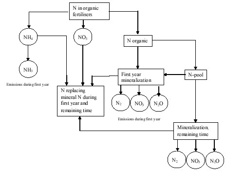
Figure D4.
Nitrogen turnover model in ORWARE (Sundqvist et al, 1999).
The nitrogen turnover sub-model gives the relation between organic fertiliser and mineral fertiliser. It is assumed that nitrogen in organic fertilisers is utilised by plants as 80 % of NH4 and NO3. Organic nitrogen is utilised to 30 % during first year after spreading compared to mineral fertiliser. Phosphorus and potassium is utilised by the plants. All metals remain in soil after spreading.
Input data to the spreading and nitrogen turnover models model in this study
- Transport distances between treatment plant and arable land is calculated as a normal transport according to transportation sub-model in ORWARE. It is assumed that organic compost and anaerobic sludge is transported with truck and trailer to arable land. No return transport is assumed.
- Calculation of acreage is based on nitrogen and phosphorus content in compost and anaerobic sludge.
- Dry spreaders spread compost.
- Anaerobic sludge is spread using liquid spreaders.
Compensatory district heating and power supply
For both electricity and heat combustion of coal is used. The same origin of data is then used for both electricity and heat combustion there is just a change of degree of efficiency between the two. In this study data from combustion of coal at the condense power plant at Fyn in Denmark is used. This plant is supposed to reflect an average type of coal condense power production plant, Uppenberg et al (1999). The coal, in the form of powder, is combusted in one older and one newer block where the newer one is equipped with semi-dry sulphur cleaning and low-NOX burner while the older block lacks of such equipment.
In Table D14 and B15 resource consumption and emission factors for power production from coal combustion is shown. Data in Uppenberg (1999) relies on the LCA for coal power (Buhre et al 1997). Uppenberg (1999) show data per MJ fuel. Coal condense power has 44 % degree of efficiency and heat and power has 88 % degree of efficiency.
Table D14.
Resource consumption for combustion of coal.
| Energy resource (MJ/MJ fuel) |
Extraction |
Use |
Sum |
| Renewable |
|
|
|
| Hydro power |
0 |
9.5E-05 |
9.5E-05 |
| Bio-fuel |
0 |
0 |
0 |
| Non renewable |
|
|
|
| Nuclear power |
0 |
1.6E-04 |
1.6E-04 |
| Natural gas |
0 |
9.24E-04 |
9.24E-04 |
| Oil |
2.32E-02 |
4.19E-03 |
2.74E-02 |
| Coal |
2.07E-02 |
5.72E-04 |
2.1E-02 |
Table D15.
Emission factors for combustion of coal expressed as g per MJ fuel.
| Emission to air |
Extraction |
Use |
Sum |
| NOx |
6.27E-02 |
0.257 |
0.32 |
| SO2 |
4.84E-02 |
0.284 |
0.33 |
| CO |
5.03E-03 |
6.23E-05 |
5.09E-03 |
| HC (NMVOC) |
1.88E-03 |
8.62E-04 |
2.74E-03 |
| CO2 fossil |
4.3 |
99 |
1.03E-02 |
| N2O |
4.17E-07 |
6.45E-07 |
1.06E-06 |
| CH4 |
8.94E-02 |
1.53E-04 |
8.96E-02 |
| Particles |
6.65E-03 |
1.19E-02 |
1.86E-02 |
Mineral fertiliser
Mineral fertilisers calculate the emissions for nitrogen (N), phosphorus (P) and potassium (K) needed to fulfil the functional unit N, P and K spread on arable land. N, P and K are calculated from Davies and Haglund (1999) using western European average data for production of mineral fertilisers. Emissions from mineral fertiliser nitrogen are calculated from spreading of Ammonium nitrate (35 % N), Western European average data. Emissions from production of phosphorus mineral fertiliser are calculated from Triple superphosphate, TSP (48 % P2O5), Western European average data and Potassium from PK fertiliser (22 % P2O5, 22 % K2O) Western European average data.
Table D16.
Resource consumption for production of mineral fertiliser N, P and K expressed as MJ per kg NPK.
| Resources |
N-tot |
P-tot |
K-tot |
| Diesel (train) |
4.37E-01 |
9.12E+00 |
5.98E-01 |
| El. European average |
3.76E-01 |
8.40E+00 |
2.57E-01 |
| Fuel, ship 2-stroke |
3.14E-02 |
1.10E+00 |
2.85E-02 |
| Hard coal |
3.95E+00 |
0 |
0 |
| Natural gas > 100 kW |
3.17E+01 |
0 |
0 |
| Oil, heavy |
4.33E+00 |
1.20E+01 |
3.14E-01 |
| Steam |
0 |
0 |
5.45E-01 |
Table D17.
Emission factors for production of mineral fertiliser N, P and K expressed as g per kg N, P and K.
| Emissions |
Nitrogen (N) |
Phosphorus (P) |
Potassium (K) |
| Cd |
2.19E-04 |
4.46E-04 |
1.19E-05 |
| Cr |
1.71E-03 |
2.10E-04 |
5.78E-06 |
| Cu |
1.57E-03 |
1.10E-03 |
3.37E-05 |
| Hg |
1.43E-05 |
6.83E-05 |
2.12E-06 |
| Ni |
5.11E-03 |
9.93E-03 |
2.70E-04 |
| Pb |
1.33E-03 |
9.31E-04 |
2.54E-05 |
| Zn |
1.75E-03 |
9.88E-04 |
2.96E-05 |
| CH4 |
2.83E+00 |
5.68E+00 |
1.80E-01 |
| CO |
1.20E+00 |
4.25E+00 |
1.67E-01 |
| CO2 |
2.84E+03 |
3.08E+03 |
1.33E+02 |
| N2O-N |
9.31E+00 |
1.83E-01 |
6.84E-03 |
| Dioxin |
6.40E-10 |
2.62E-09 |
8.20E-11 |
| NMVOC |
1.24E+00 |
6.49E+00 |
2.19E-01 |
| NH3-N |
0 |
1.20E-03 |
3.44E-05 |
| NO2-N |
4.11E+00 |
0 |
0 |
| NOx-N |
1.42E+00 |
5.58E+00 |
2.10E-01 |
| N-tot |
1.48E+01 |
5.76E+00 |
2.17E-01 |
| PAH |
3.20E-04 |
6.01E-06 |
5.94E-06 |
| SO2-S |
2.20E+00 |
1.92E+01 |
5.26E-01 |
| SO3-S |
0 |
5.31E-01 |
1.38E-02 |
| S-tot |
2.20E+00 |
1.97E+01 |
5.40E-01 |
| Cd (aq) |
7.77E-06 |
3.76E-05 |
1.20E-06 |
| Cr (aq) |
8.51E-06 |
2.10E-04 |
6.57E-06 |
| Cu (aq) |
2.80E-06 |
5.82E-05 |
2.42E-06 |
| Ni (aq) |
6.20E-05 |
2.43E-04 |
7.65E-06 |
| Pb (aq) |
5.80E-05 |
2.74E-04 |
8.69E-06 |
| COD (aq) |
1.72E-03 |
3.51E-02 |
1.45E-03 |
| P-tot (aq) |
3.43E-06 |
3.30E+00 |
8.64E-02 |
| SO4-S (aq) |
2.34E-01 |
2.33E+00 |
7.18E-02 |
| S-tot (aq) |
2.34E-01 |
2.33E+00 |
7.18E-02 |
| BOD (aq) |
6.86E-05 |
1.09E-03 |
4.50E-05 |
| Front page | | Contents | | Previous | | Next | | Top |
|