|
| Front page | | Contents | | Previous | | Next |
The Influence of Sorption on the Degradation of Pesticides and other Chemicals in Soil
6 The influence of sorption on the degradation described by mathematical models
It has often been seen that the sorption has a limiting effect on the degradation rate of pesticides, which can be explained by the fact that first of all it is the amounts of pesticide available in the aqueous phase of the soil that can be microbially degraded. Even though this factor plays a part, a degradation of sorbed chemicals may still take place to a certain extent. If the desorption is dependent on time and takes place at a rate that is on a level with or lower than the degradation rate, the dependence of the degradation on the sorption leads to complex kinetics even though the degradation kinetics itself is simple first-order kinetics. Guo et al. (2000) studied the influence of the sorption on the degradation rate of 2,4-D in the presence of varying amounts of activated carbon and described the sorption by a two-compartment first + first-order degradation process which took place in the aqueous phase and in the sorbed phase, respectively. Guo concluded that the degradation process took place in the two phases at different rates.
Hill and Schaalje (1985) described a two-compartment model for the degradation of deltamethrin in soil. Jones et al. (1996) and Reid et al. (2000) pointed out that curves (Figure 5) that describe the course of the degradation
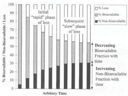
Figure 5. A biphasic degradation process for a chemical in soil (Reid et al., 2000). The figure is reproduced with the kind permission from Elsevier.
Figur 5. Et to-faset nedbrydningsforløb for et kemisk stof i jord (Reid et al, 2000). Figuren er gengivet med tilladelse fra Elsevier.
of chemicals in soil often consist of two phases, an initial phase with a quick degradation and a second phase with a much slower degradation, where they were of the opinion that the relative significance of each of these phases would be determined by the volatility and hydrofobicity of the chemical. If the degradation takes place according to such a biphasic process, it is not logical to determine the degradation of chemicals by means of half-lives. Using 14C-labelled substances and measurement of the formed 14CO2, Scow et al. (1986) analysed the kinetics of the mineralisation of chemicals in soil and pointed out that this, too, was a two-phase process (Figure 6). Fomsgaard and Kristensen (1999a, 1999b) and Fomsgaard (1999) described the biphasic mineralisation of ETU with mathematical models, which were able to describe processes both with and without microbial growth (Figure 7), and stated, just like Scow (1986) and Brunner and fOC ht (1984), that the second – considerably slower – phase of the mineralisation process had to be a mineralisation of the soil organic matter in which 14C from the pesticide had already been built in or to which it had already been strongly bound. Whether - in the second phase - it is in actual fact a question of 14C being first built into the soil organic matter, which subsequently is mineralised, or whether a slow mineralisation takes place of the foreign chemical molecule that is bound to the surface of the soil is difficult to tell. If measurable amounts can be extracted when the mineralisation experiment is interrupted, then the latter is the case. In the cases in the studies of Fomsgaard and Kristensen (1999a, 1999b) where the mineralisation in the first compartment took place with no-growth kinetics, a two-compartment first + first-order process was the model which resulted in the best fit of the mineralisation.
Figure 6. Biphasic mineralisation curve for aniline in varying concentrations (from Scow et al., 1986). The figure is reproduced with the kind permission from American Society for Microbiology.
Figur 6. To-faset mineraliseringskurve for anilin i varierende koncentrationer (fra Scow et al, 1986). Figuren er gengivet med tilladelse fra American Society for Microbiology.
Figure 7. Two-compartment mineralisation of 14C-ETU (Fomsgaard, 1999).
A. Data points ......... and model ________:
B. Data points ......... and the first term of the model______:
C. Data points........ and the second term of the model_____:

Figur 7. To-compartment mineralisering af 14C-ETU (Fomsgaard, 1999).
A. Datapunkter ......... og model ________:
B. Datapunkter ......... og første led af modellen______:
C. Datapunkter........ og andet led af modellen_____:
Sjelborg et al. (2002a) compared the use of a one-compartment first-order model and a two-compartment first + first-order model respectively for the description of the degradation of ioxynil: The models were described as
| first-order model: |
c(t) = a·e-k1·t |
| first + first-order model: |
c(t) = a·e-k1·t + b·e-k2·t |
| where |
| c(t) = the amount of remaining pesticide at the time t |
| a = the initial amount of pesticide degraded according to the initial first-order process |
| b = the initial amount of pesticide degraded according to the second first-order process |
| t = the time in days |
| k1 = rate constant for the degradation in the first compartment |
| k2 = rate constant for the degradation in the second compartment |
The comparison of the application of the two different models is seen in Figure 8. A first-order degradation process can be solved analytically, and a half-life (DT50) can be determined. A two-compartment first + first-order process cannot be solved analytically, and it was concluded that the use of a half-life, calculated from the simple first-order process, for a description of degradation rates is not adequate.
Many mathematical models, which were formerly used to describe the degradation kinetics of a chemical, took as their starting points the degradation of a single soluble chemical by means of a single culture of bacteria in a suspended experimental system. One of the models, which were often used where bacterial growth occurs, is the Monod model. From this, various other models can be derived for describing the degradation of a substance, each of these models having its own relevance depending on the initial concentration of the chemical and the bacterial density – models such as first-order, zero-order, Michalis-Menten, logarithmic, and logistic equations (Simkins & Alexander, 1984). As to chemicals in soil, first and foremost pesticides, it is frequently assumed that the degradation takes place according to simple first-order kinetics from which a DT50 -value is derived. Scow et al. (1986) and Fomsgaard (1999) showed that the mathematical description of mineralisation curves, in which the 14CO2 development from 14C-labelled pesticide is measured, is best carried out by means of two-term models where the second term describes the slow degradation of 14C from the pesticide, which has been built into or strongly bound to the soil constituents.
Many authors have been of the opinion that a degradation that was much slower than expected is due to a slow diffusion of the chemical through the soil matrix before it reaches the microorganisms (Gustafson & Holden, 1990; Firestone, 1982; fOC ht & Shelton, 1987; Myrold & Tiedje, 1985; Schmidt & Gier, 1989). Pignatello (1989), Harmon et al. (1989), Brusseau and Rao (1989), and Brusseau et al. (1991) showed that diffusion is the process that dominates sorption and desorption processes. Scow and Hutson (1992) and Scow and Alexander (1992) developed a diffusion-sorption-biodegradation model (DSB) and applied it to empirical experiments. The model is outlined schematically in Figure 9. The results show that in suspensions of soil in water or if the soil aggregates are very small or when the concentration in the solution is very large a simple first-order process can often be used to describe the degradation of chemicals in soil. But if systems are involved where the
Figure 8. Application of first-order and two-compartment first-order model, respectively, for description of the degradation of ionynil (0.5 mg/kg) in plough layer soil and soil from a depth of 80-100 cm from Faardrup. The points are the experimental values whereas the full-drawn line is the mathematical model (Sjelborg et al., 2002a).
Figur 8. Anvendelse af 1. ordens henholdsvis to compartment 1. ordens model til beskrivelse af nedbrydningen af ioxynil (0,5 mg/kg) i pløjelagsjord og jord fra 80-100 cm fra Faardrup. Punkterne er de eksperimentelle værdier, mens den fuldt optrukne linje er den matematiske model (Sjelborg et al., 2002a).
water content of the soil is natural, if large aggregates are present or when the concentration in the soil water is small, a two-compartment model must be used to describe the degradation, and the rate constant for the slow part of the two-compartment degradation and the distribution of the amount of pesticide on the two degradation processes are determined by the diffusion/sorption of the substance in the soil (Scow & Hutson, 1992). Shelton and Doherty (1997a, 1997b) described a combined sorption-degradation model, which involved growth kinetics of the degradation process and used it for describing the decomposition of 2,4-D in soil. Gamerdinger et al. (1990) and Beigel et al. (1999) developed models that described the simultaneous sorption and degradation of chemicals in soil that could be used for studies, which were carried out as leaching experiments in small columns.
Figure 9. Schematic diagram showing the relation in the diffusion-sorption-biodegradation model (Scow & Hutson, 1992). The figure is reproduced with the kind permission from Soil Science of American Journal.
Figur 9. Skematisk diagram, der viser sammenhængen i diffusion-sorption-bionedbrydningsmodellen (Scow og Hutson, 1992). Figuren er gengivet med tilladelse fra Soil Science of American Journal.
Sjelborg et al. (2002b) compared the degradation of fenpropimorph in three different soils that had been incubated with the substances in the concentration of 0.5 mg/kg and with a natural water content and described the degradation by a two-compartment first + first-order process and a simple first-order process respectively (Figure 10 – Figure 12). It was entirely consistent that the description by the two-compartment model resulted in a higher correlation coefficient than the description by the simple first-order model (see the values in Figures 10 – 12). As in the literature mentioned above, the two compartments can be regarded as one compartment where a relatively quick decomposition of freely available pesticide takes place and another compartment where the decomposition is slower because it is controlled by a desorption or diffusion process. The distribution of the amounts of pesticides a and b between the two compartments is apparently determined by the structure of the pesticide, the amount of present organic matter to which the substance can be bound, and the rate k1 at which some of the pesticide can be decomposed in the first compartment before the
Figure 10. Degradation of phenpropimorph Faardrup 0-20 cm. a) Two-compartment first + first-order model. b) First-order model. Points: data points. Full-drawn line: model. Correlation coefficient r2. Half-life according to the first-order model = 15 days. The first three half-lives according to the first + first-order model: 4.2 days, 21.8 days, and 35.8 days, respectively (Sjelborg et al., 2002b)
Figur 10. Nedbrydning af fenpropimorph Fårdrup 0-20 cm. a) to-compartment 1.+1. ordens model. b) 1. ordens model. Punkter: datapunkter. Fuld optrukken linje: model. Korrelationskoefficient r2 . Halveringstid ifølge 1. ordens modellen = 15 dage. De første tre halveringstider ifølge 1.+1. ordens modellen: 4,2 dage, 21,8 dage and 35,8 dage (Sjelborg et al., 2002b).
Figure 11. Degradation of phenpropimorph Jyndevad 0-20 cm. a) Two-compartment first + first-order model. b) First-order model. Points: data points. Full-drawn line: model. Correlation coefficient r2. Half-life according to the first-order model = 122.6 days. The first three half-lives according to the first + first-order model: 66.3 days. The following half-lives cannot be calculated (Sjelborg et al., 2002b).
Figur 11. Nedbrydning af fenpropimorph Jyndevad 0-20 cm. a) to-compartment 1.+1. ordens model. b) 1. ordens model. Punkter: datapunkter. Fuld optrukken linje: model. Korrelationskoefficient r2 . Halveringstid ifølge 1. ordens modellen = 122,6 dage. De første tre halveringstider ifølge 1.+1. ordens modellen: 66,3 dage. De følgende halveringstider kan ikke beregnes (Sjelborg et al., 2002b).
Figure 12. Degradation of phenpropimorph Tylstrup 0-20 cm. a) Two-compartment first + first-order model. b) First-order model. Points: data points. Full-drawn line: model. Correlation coefficient r2. Half-life according to the first-order model = 379 days. The first three half-lives according to the first + first-order model: 483 days, 623 days, and 624 days, respectively (Sjelborg et al., 2002b).
Figur 12. Nedbrydning af fenpropimorph Tylstrup 0-20 cm. a) to-compartment 1.+1. ordens model. b) 1. ordens model. Punkter: datapunkter. Fuld optrukken linje: model. Korrelationskoefficient r2 . Halveringstid ifølge 1. ordens model = 379 dage. De første tre halveringstider ifølge 1.+1. ordens modellen: 483 dage, 623 dage og 624 dage (Sjelborg et al., 2002b).
remaining amount is bound in the second compartment. The rate of the degradation process in the first compartment k1 is probably determined by the biological activity whereas the rate of process in the second compartment k2 is determined by the desorption/diffusion rate. A model describing these relations is being prepared.
In a two-compartment first + first-order equation the DT50-value cannot be found analytically; half-lives can only be indicated from readings of the curve or from an iterative method. The simple first-order equation, on the other hand, can be solved analytically as DT50 = ln2/k. The half-life according to the first-order equation is therefore the same no matter where one is in the process whereas the half-life according to the two-compartment first + first-order process changes over time and typically lengthens as the rate constant for the degradation is low in the second compartment, which becomes the dominant one as time passes.
In the leaching model, MACRO, a possibility is built in of inserting two DT50-values for the aqueous phase of the soil and the sorbed phase respectively. The normal procedure is to insert the same DT50-value in both phases, which has been calculated on the basis of a simple first-order process. However, on the basis of the two-compartment model a half-life for each of the two compartments can be calculated from ln2/k, and the distribution of the of substance can be taken into account. In this way, one can assess the application of the two degradation models. However, a developed version of MACRO of which a model description combining the sorption and the degradation processes forms part would be preferable by far.
The error that is made by using a simple first-order model as the basis for calculations of half-lives varies according to the other circumstances in the soil. In Figure 10 is seen that the half-life is estimated at 15 days according to the simple first-order process whereas it is just 4.2 days for the first halving according to the two-compartment model. If one assumes that the part of the substance that is decomposed in the second compartment has been extracted only owing to the application of an organic extraction agent and that it will not otherwise be available to the biology of the soil or to leaching to the groundwater, then a more severe assessment of the substance has been made when using the simple first-order process than might be considered reasonable. On the other hand, if the amount that is decomposed in the second compartment in actual fact is bioavailable or can be leached to the groundwater, the substance is assessed too mildly when using the simple first-order process as three halvings are estimated at just 45 days whereas it takes 62 days according to the two-compartment process. Thus it is not just a question of a need to find the right model for describing the sorption-degradation process but also a question of throwing light upon the type of binding and the bioavailability of the amounts of the substance that are decomposed in the second compartment.
Sorensen et al. (1998) ranked the results of a number of monitoring findings of leached pesticides, compared this ranking with the ranking of various descriptors for the pesticides, and showed that there was a close connection between the ranking according to monitoring data and the ranking according to the three descriptors, dosage, sprayed area, and KOC-value. On the other hand, the ranking in relation to the DT50-value was not nearly so usable in relation to the found monitoring data. The ranking in relation to the degradation rate might have been more usable if a two-compartment model had been used for the description of the degradation.
| Front page | | Contents | | Previous | | Next | | Top |
Version 1.0 March 2004, © Danish Environmental Protection Agency
|