Pesticides Research no. 64, 2004
Technical Documentation of PestSurf, a Model describing Fate and Transport of Pesticides in Surface Water for Danish Conditions
Contents
1 Technical Background Information
- 2.1 Wind drift
- 2.2 Deposition of soil surfaces
- 2.3 Dry deposition
- 2.4 Colloid transport
- 2.5 Transport and transmission process in the streams and ponds
- 2.5.1 Sedimentation and resuspension
- 2.5.2 Diffusive exchange between water column and sediment in the rivers
- 2.5.3 Diffusive exchange between water column and sediment in ponds
- 2.5.4 Sorption to particles in water column and sediment
- 2.5.5 Sorption to macrophytes
- 2.5.6 Biodegradation of active substances
- 2.5.7 Photolytic degradation of active substances
- 2.5.8 Hydrolysis
- 2.5.9 Evaporation
- 3.1 How to start the system
- 3.2 The system
- 3.3 General Menu-pages
- 3.3.1 Basic parameters
- 3.3.2 Catchment and type of surface water
- 3.3.3 Crop
- 3.3.4 Width of protection zone
- 3.3.5 Spraying data
- 3.3.6 Basic chemical and physical properties of the active substance (and metabolite)
- 3.3.7 Sorption of active substance in soil
- 3.3.8 Degradation of active substance in soil
- 3.3.9 Sorption of active substance in surface water
- 3.3.10 Aerobic degradation of active substance in surface water
- 3.3.11 Anaerobic degradation of active substance in surface water
- 3.3.12 Hydrolysis of active substance in surface water
- 3.3.13 Photolysis of active substance in surface water
- 3.3.14 Pesticide transformations to metabolite
5 Statistical Functions Included
Appendix A - Measured and Fitted Wind Drift Curves
Appendix B - Tsf- and xtsf-file Samples
Appendix C - Examples of *.ad11, *.PE11 files used for MIKE 11
Appendix D - Basic Soil Data for Calculation of T2-files Required for the Setup
Appendix E - Application of Pesticide Diffusion in Sediments to MIKE 11
Appendix F - Sediment compostion
Appendix G - Calculation of biodegradation
Preface
The project "Model Based Tool for Evaluation of Exposure and Effects of Pesticides in Surface Water", funded by the Danish Environmental Protection Agency (DEPA), was initiated in 1998. The aim of the project was:
To develop a model-based tool (PestSurf) for evaluation of risk related to pesticide exposure of surface water. The tool must be directly applicable by the Danish Environmental Protection Agency in their approval pr°Cedure. As part of this goal, the project had to:
- Develop guidelines for evaluation of meSocosm experiments based on a system-level perspective of the fresh water environment
- To develop models for deposition of pesticides on vegetation and soil.
- To estimate the deposition of pesticides from the air to the aquatic environment.
The project, called "Pesticides in Surface Water", consisted of seven subprojects with individual objectives. The sub-projects are listed in Table 1.
Table i Sub-projects of "Pesticides in Surface Water"
Tabel i Oversigt over delprojekter i "Pesticider i overfladevand"
| Title | Participating institutions | |
| A | Development and validation of a model for evaluation of pesticide exposure | DHI Water & Environment (DHI) |
| B | Investigation of the importance of plant cover for the deposition of pesticides on soil | Danish Institute of Agricultural Sciences (DIAS) |
| C | Estimation of the airborne transport of pesticides to surface water by dry deposition and spray drift | National Environmental Research Institute (NERI) Danish Institute of Agricultural Sciences (DIAS) |
| D | Facilitated transport | DHI Water & Environment |
| E | Development of an operational and validated model for pesticide transport and fate in surface water | DHI Water & Environment
National Environmental Research Institute |
| F | MeSocosm | DHI Water & Environment
National Environmental Research Institute (NERI) |
| G | Importance of different transport routes in relation to occurrence and effects of pesticides in streams | National Environmental Research Institute (NERI)
County of Funen County of Northern Jutland |
Figure 1 Links between the different sub-projects. The sub-projects are placed on a cross-section of the catchment to illustrate interactions
Figur 1 Sammenhæng mellem delprojekterne. Delprojekterne er placeret på et tværsnit af en opland for at illustrere interaktionerne
Figure 1 describes the relationship between the sub-projects. Sub-project 1 models the upland part of the catchment, while sub-project 5 models surface water bodies. Sub-project 8 delivers data to both modelling projects. Sub-project 2 and 3 develop process descriptions for spray drift, dry deposition and deposition on soils. Sub-project 4 builds and tests a module for calculation of colloid transport of pesticide in soil. The module is an integrated part of the upland model. Sub-project 6 has mainly concentrated on interpretation of meSocosm-studies. However, it contains elements of possible links between exposure and biological effects.
The reports produced by the project are:
- Styczen, M., Petersen, S., Christensen, M., Jessen, O.Z., Rasmussen, D., Andersen, M.B. and Sørensen, P.B. (2004): Calibration of models describing pesticide fate and transport in Lillebæk and Odder Bæk Catchment. - Ministry of Environment, Danish Environmental Protection Agency, Pesticides Research No. 62.
- Styczen, M., Petersen, S., Sørensen, P.B., Thomsen, M and Patrik, F. (2004): Scenarios and model describing fate and transport of pesticides in surface water for Danish conditions. - Ministry of Environment, Danish Environmental Protection Agency, Pesticides Research No. 63.
- Styczen, M., Petersen, S., Olsen, N.K. and Andersen, M.B. (2004): Technical Documentation of PestSurf, a model describing fate and transport of pesticides in surface water for Danish Conditions. - Ministry of Environment, Danish Environmental Protection Agency, Pesticides Research No. 64.
- Jensen, P.K. and Spliid, N.H. (2003): Deposition of pesticides on the soil surface. - Ministry of Environment, Danish Environmental Protection Agency, Pesticides Research No. 65.
- Asman, W.A.H., Jørgensen, A. and Jensen, P.K. (2003): Dry deposition and spray drift of pesticides to nearby water bodies. - Ministry of Environment, Danish Environmental Protection Agency, Pesticides Research No. 66.
- Holm, J., Petersen, C., KOCh, C. and Villholth, K.G. (2003): Facilitated transport of pesticides. - Ministry of Environment, Danish Environmental Protection Agency, Pesticides Research No. 67.
- Helweg, C., Mogensen, B.B., Sørensen, P.B., Madsen, T., Rasmussen, D. and Petersen, S. (2003): Fate of pesticides in surface waters, Laboratory and Field Experiments. Ministry of Environment, Danish Environmental Protection Agency, Pesticides Research No. 68.
- Møhlenberg, F., Petersen, S., Gustavson, K., Lauridsen, T. and Friberg, N. (2001): Guidelines for evaluating meSocosm experiments in connection with the approval pr°Cedure. - Ministry of Environment and Energy, Danish Environmental Protection Agency, Pesticides Research No. 56.
- Iversen, H.L., Kronvang, B., Vejrup, K., Mogensen, B.B., Hansen, A.M. and Hansen, L.B. (2003): Pesticides in streams and subsurface drainage water within two arable catchments in Denmark: Pesticide application, concentration, transport and fate. - Ministry of Environment, Danish Environmental Protection Agency, Pesticides Research No. 69.
The original thoughts behind the project are described in detail in the report "Model Based Tool for Evaluation of Exposure and Effects of Pesticides in Surface Water", Inception Report – J. nr. M 7041-0120, by DHI, VKI, NERI, DIAS and County of Funen, December, 1998.
The project was overseen by a steering committee. The members have made valuable contributions to the project. The committee consisted of:
- Inge Vibeke Hansen, Danish Environmental Protection Agency, (chairman 1998-mid 2000).
- Jørn Kirkegaard, Danish Environmental Protection Agency (chairman mid-2000-2002).
- Christian Deibjerg Hansen, Danish Environmental Protection Agency.
- Heidi Christiansen Barlebo, The Geological Survey of Denmark and Greenland.
- Mogens Erlandsen, University of Aarhus.
- Karl Henrik Vestergaard, Syngenta Crop Protection A/S.
- Valery Forbes, Roskilde University.
- Lars Stenvang Hansen, Danish Agricultural Advisory Centre (1998-2001).
- Poul-Henning Petersen, Danish Agricultural Advisory Centre (2002).
- Bitten Bolet, County of Ringkøbing (1988-1999).
- Stig Eggert Pedersen, County of Funen (1999-2002).
- Hanne Bach, The National Environmental Research Institute (1999-2002).
October 2002
Merete Styczen, project co-ordinator
Sammenfatning og konklusioner
PestSurf er et værktøj, der har til formål at udføre pesticidsimuleringer til vurdering af plantebeskyttelsesmidlers forventede påvirkning af nærliggende overfladevand. Værktøjet består af en række programdele, der tilsammen udfører de nødvendige beregninger.
Værktøjets kerne er fire modelopsætninger med MIKE SHE (hydrologisk oplandsmodel) og MIKE 11 (model for vandløb og vandhuller). Oprindeligt er disse modeller opstillet for et moræneområde (Lillebæk) og et mere sandet område (Odder Bæk). Disse to oprindelige modeller indgår i let modificeret form som grundlæggende scenarier. I hver af de to områder er indført et vandhul, sådan at der kan simuleres enten et vandløb eller et vandhul for hvert typeområde.
Alle parametre, der ikke er pesticidrelevante, er låst i modelopsætningerne. Brugeren kan imidlertid, gennem værktøjets brugerflade, vælge hvilken modelopsætning, beregningerne skal foretages på, indføre det aktuelle pesticids egenskaber, vælge beskyttelseszoner og køre modellen.
Når modellen igangsættes, omregnes de angivne værdier til de relevante modelparametre, og vinddrift og tørdeposition beregnes og skrives ind i tidsseriefiler, der tilføres vandløbsmodellen direkte. Afhængigt af hvilken afgrøde, der udføres scenarie-beregninger for, hentes en forberegnet fil med de nødvendige vandstrømninger. PestSurf gennemfører derfor kun de ønskede stofberegninger.
Rapporten indeholder den tekniske dokumentation for de processer, der ikke findes i de eksisterende MIKE SHE- og MIKE 11-manualer, nemlig vinddrift, tørdeposition, beregning af doseringen, der rammer jordoverfladen, kolloidtransport og pesticidrelevante processer i vandløb og vandhuller. Desuden findes en beskrivelse af modellens brugerflade.
Kalibreringen af modellerne samt de anvendte scenarier er beskrevet andetsteds.
Summary and conclusions
PestSurf is a tool developed with the purpose of carrying out simulations to assess the expected effects of an active substance on adjacent surface water bodies. The tool consists of a number of programme modules, which together carries out the necessary calculations.
The kernel of the tool is four model setups of MIKE SHE (hydrological catchment model) and MIKE 11 (model for streams and ponds). Originally, these models were made for a moraine clay area (Lillebæk) and a more sandy area (Odder Bæk). These two original models in a slightly modified form are contained as the basic scenarios. In each of the two areas, a pond is created to make it possible to simulate either a stream or a pond for each type of area.
All parameters, which are not of relevance for active substance simulations, are l°Cked in the model. However, the user can, through the user interface of the tool, choose which model setup the calculations must be based on, enter the properties of the active substance, choose a buffer zone and run the model.
When PestSurf is started, the input values entered are recalculated to model parameters, and wind drift and dry deposition is calculated and written to time series files, specifying the actual input to the stream model. Depending on which crop the calculations are carried out on, a pre-calculated file with the required water fluxes is selected. PestSurf only governs the calculation of solute transport and transformation.
The report contains the technical Documentation for the processes not described in the existing MIKE SHE and MIKE 11-manuals, that is wind drift, dry deposition, calculation of the dosage hitting the soil surface, colloid transport and processes of relevance for transport and transformation of the active substance in streams and ponds. Furthermore, the user interface is described.
The calibration of the models and the selected scenarios are described elsewhere.
1 Technical Background Information
PestSurf is a model for estimation of transport of active substance to streams and ponds. It is build with the model systems MIKE SHE (Refsgaard and Storm, 1995) and MIKE 11 (DHI, 1997). The two model systems has been implemented on two Danish catchments (Styczen et al., 2004a), and these calibrations form the base for the scenarios (Styczen et al., 2004b) that can be simulated by PestSurf. The PestSurf interface allows the user to select a pond or a stream in either of the two scenario catchments, and parameterise an active substance and/or a metabolite.
This Documentation concentrates on the differences between the models included in "PestSurf" and the standard models MIKE SHE and MIKE 11. It is not the intention to repeat the information already available in the User manuals of MIKE SHE and MIKE 11. These Documents will be made available to the Environmental Protection Agency together with the model. The relevant Documents and the topics of particular relevance to "PestSurf" are listed in Table 1.1.
Table 1.1 Documentation available in MIKE SHE and MIKE 11 User Manuals.
Tabel 1.1 Dokumentation tilgængelig i MIKE SHE og MIKE 11-brugermanualer.
| Technical Documents | Topics |
| MIKE SHE Water Movement, User manual |
- Overland Flow Module, MIKE 11 Channel Flow Module
- MIKE SHE ET – Evapotranspiration Module - Unsaturated Zone Module – Richards Eq. - Wetland Infiltration and Evapotranspiration Module - Saturated Zone Flow Module –2D/3D Finite Difference Model - Snow Melt Module - Vegetation Database Manual - Simulation Control Module |
| MIKE SHE Water Quality,
User manual |
- Advection-Dispersion Module
- The sorption-degradation module described in this manual is the base on which the updated version (Section 2.4) is made. |
| MIKE SHE Agriculture,
User manual |
- Macropore module |
| MIKE 11 | - hydrodynamic module
- advection-dispersion module |
2 New process Descriptions
In comparison to the standard-version of the MIKE SHE and MIKE 11 models, different components have been added. Some of these are added as pre-processing of data, while some are added directly into the model processes. The calculations performed and the formulas used, are described in the sub-sections of this chapter.
The new components are:
- wind drift (Asman et al., 2003)
- dry deposition (Asman et al., 2003)
- Deposition on the soil surface (Jensen and Spliid, 2003)
- colloid transport (Holm et al., 2003)
- pesticide-related processes in the river (described in this report, but based on work of Helweg et al., 2003)
2.1 Wind drift
The considerations, on which the choice of description is made, are described in Asman et al. (2003). Drift is described for agricultural crops, fruit trees and spruce trees.
For agricultural crops, the values of the Ganzelmeier-kurve (ref) corresponding to 95% drift is selected to represent average drift conditions for Denmark. Apple trees represent fruit trees. Spruce trees, when small, are sprayed from above, and the drift is therefore considered similar to agricultural crops. When the trees are larger, they are sprayed from the side, and to mimic this situation, the drift value is calculated as the average of drift for late and early hops. The values, on which the drift calculations are based, are given in Table 2.2.
Curves were fitted to each dataset. The relationships are
For agricultural crops:
Y = exp(ln(B) +β*x – x*A*e(α*x)) (Eq. 1)
where
x = distance
y = Drift as % of dosage
and the constants are give below:
| X<7.5 m | x>=7.5 m | |
| B | 25.6979 | 1.6195 |
| A | 2.7528 | 0.6745 |
| β | -0.4831 | 0.4709 |
| α | -0.6020 | -0.0061 |
The relationship allows x = 0, and fitted better than simpler relationships investigated.
For apples:
Y = B * Eax (Eq. 2)
Before leaves occur (before 1st of June)
if x<15, a=-0.127 and b = 39, else a=-0.102 and b = 31
After leaves has occurred, (after 1st of June)
if x <10, a = -0.1966 and b = 28; else 1= -0.0996 and b=11
For spruce:
Y = (29.35*exp(-3.07*log(x)) + 19.66 * exp(-3.56*log(x)))/2 (Eq. 3)
equal to the average of the fittings of early and late hops.
Figures showing measured data and fitted curves are shown in Appendix A.
The distance, x, is expected to consist of a distance from the sprayer to the stream, the buffer zone and half the width of the stream. The width of the stream is, in average, 1.3 m for Odder Bæk and 40 cm for Lillebæk. Half the width of the stream is therefore 0.65 and 0.2 m, respectively.
Table 2.1. The distance from the sprayer to the centre of the stream.
Tabel 2.1. Afstanden fra sprøjtedyssen til centeret af vandløbet.
| Crop | Distance from sprayer to stream | Buffer zone | Half river width |
| Agricultural crops | 0.0 m | 0-50 m | 0.2 or 0.65 m |
| Apple trees | 3.0 m | 0-50 m | 0.2 or 0.65 m |
| Spruce trees (sideways) | 1.5 m | 0-50 m | 0.2 or 0.65 m |
Each of the streams are divided into five segments (Styczen et al., 2004b, p. 43), and drift is calculated for each of these segments, taking into account the width of the buffer zone for each segment (For the pond, only one calculation is made). The amount is then recalculated to mass per stream segment, assumed to be sprayed into the river over 30 minutes. The resulting time series form direct input to the river model. For each spraying event, the drift from the whole length of stream is added over the same 30 minutes.
The implicit assumption is that the wind is always perpendicular to the stream, and blowing with a constant velocity. However, spray drift is added from one side of the water body only.
Table 2.2. Drift values, on which the drift calculations (equation 1-3) are based. The data are from BBA (2000)
Tabel 2.2. De vinddrift-værdier, der er basis for de udledte ligninger (ligning 1-3). Data stammer fra BBA (2000)
| Dist, m | Deposition, % of appl. Dose Agricultural crops |
Apples | Vines | ||
| Early stages | Late stages | Early | Late | ||
| 1 | 3.51 | ||||
| 2 | 1.24 | ||||
| 3 | 0.98 | 29.6 | 15.5 | 3.6 | 6.78 |
| 4 | 0.94 | ||||
| 5 | 0.75 | 19.5 | 10.1 | 1.63 | 3.43 |
| 7.5 | 0.42 | 14.1 | 6.4 | 0.87 | 2 |
| 10 | 0.33 | 10.6 | 4.4 | 0.55 | 1.36 |
| 15 | 0.2 | 6.2 | 2.5 | 0.29 | 0.79 |
| 20 | 0.12 | 4.2 | 1.4 | 0.19 | 0.54 |
| 30 | 0.11 | 2 | 0.6 | ||
| 40 | 0.4 | ||||
| 50 | 0.2 | ||||
The process is executed as part of the data transformation that takes place when input data given by the user is transformed to model input, and may thus be considered pre-processing.
2.2 Deposition of soil surfaces
The theoretical works, on which the relationships are based, are described in Jensen and Spliid (2003). The deposition on the soil is estimated in two different ways, for the situation with and without a plant cover.
For early sprayings, the plant cover is set to zero. The dose only has to be corrected for losses due to drift and dry deposition.
The total mass of dry deposition and spray drift to the stream is calculated, and deducted from the total mass of active substance sprayed. The result is divided by the sprayed area to calculate a slightly reduced average dose.
When a crop cover (> 20) is present, the dose is corrected for wind drift losses, and the deposition on soils is calculated as the corrected dose times a fraction. The fraction depends on the crop and the crop stage. The values as function of crop and time are shown in Appendix A of Styczen et al. (2004b).
In this case, the dry deposition is calculated based on emission from leaves, and the dose hitting the ground should therefore not be corrected for this loss.
In the test cases carried out, the corrections for drift and dry deposition on the average dose is less than 1%.
The resulting dose to the ground is transformed into a time series file (Spraying_corr.T0), where the dosage is repeated every year at the specified date, or, if the user specifies that spraying during rain is not allowed, the spraying date is moved forward until the criteria is fulfilled. The time series file is applied to the agricultural area of the catchment. This area is described by the file "Catchmentname_stream/pond_agrl0.T0" or "Catchmentname_stream/pond_agrl35.T0, depending on whether the buffer zone is below or above 35 meters.
The process is executed as part of the data transformation that takes place when input data given by the user is transformed to model input, and may thus be considered pre-processing. The names of the spraying file and the file describing the area to be sprayed are then transferred to the *.tsf-file (Catchmentname_stream/pond_pesticide/metabolite.tsf) that is part of the input to the MIKE SHE active substance simulation.
2.3 Dry deposition
The theoretical basis for the description of dry deposition is given in Asman et al. (2003). The description is a separate model entity, called PestDep, which is called by the pre-processing programme that transforms data from the interface.
In the model the wind direction (x direction) is always perpendicular to the water body (y direction). The deposition is assumed to be the same everywhere in the y direction along the river (in the model the river and the emission field are indefinitely long in this direction). The z direction is the vertical. The wind is always blowing from the emission area to the water body. Although this sounds unrealistic, it is in fact not so unrealistic because there are usually fields on both sides of the water body. Of cause the wind cannot blow pendicular to the entire length of a twisted and bended river. This was taken in to account through calculation of an effective exposed length of the river, calculated through projection of the river stretch on to straight line connecting the upper and lower end of the river (see Styczen et al., 2004b, section 4.2). Part of the time the wind will be blowing along the water body. This situation is not taken into account. In this way a maximum dry deposition to the water body is calculated.
The model version described here is made for streams and small ponds, not for large water bodies, such as seas.
In general, the programme is parameterised via the interface and the pre-processing programme. As for the drift calculations, time series are prepared for five segments of each river stretch. For the ponds, only one time series is prepared.
A number of parameters are given default values, or general values of relevance to the catchments. These are listed in Section 2.3.5.
2.3.1 Emission
The model distinguishes between emission from bare soil and a crop cover.
In the input file the indicator indicvol indicates the type of volatilisation calculation that has to be made:
- If indicvol = 1, the accumulated emission after application to crops during 7 days is calculated. In that case the parameters necessary for the calculation of the accumulated emission after application to normal moist fallow soil are read, but not used.
- If indicvol = 2, the accumulated emission after application to normal moist fallow soil during 21 days is calculated. In that case the parameters necessary for the calculation of the accumulated emission after application to crops are read, but not used. If the fraction of the active substance in the gas phase in the soil is outside the range for which the accumulated emission can be calculated a value of 0 is given (otherwise e.g. negative emissions will be generated).
The length of the emission zone in the x direction (downwind direction, perpendicular to the water body) is needed to calculate the absolute emission for the whole emission zone. It is calculated as: the 0.5*(total area of the catchment minus the area upstream of the upper end of each stream), divided by the length of the stream, measured as projections of the stream on to a straight line between the upper and lower end of the river (see Styczen et al., 2003b, section 4.2).
2.3.1.1 Emission from crops
Input data:
- Dose (kg active ingredient ha-1). To take into account that the compound may be non-neutral, the amount of neutral species is calculated using the pKa-value of the compound, assuming a pH of 7.
- Vapour pressure at a reference temperature (Pa).
- Reference temperature vapour pressure (K).
- Actual temperature of the crop (K). It is set to the actual air temperature that is read in the input file.
The dose and the vapour pressure comes from the interface while the reference temperature is assumed to be 20 C° (= 293.16 K). The actual temperature is read as the air temperature of the day that the spraying takes place.
Output data:
- Accumulated emission during 7 days (% of the dose).
The accumulated emission of active substances during 7 days after application to crops is calculated with the equation
10log(CV7)=1.528+0.466 10log(VP); for VP≤ 10.3 mPa (Eq. 4)
where:
CV7 = accumulated emission during 7 days after application (% of dosage of active ingredient).
VP = vapour pressure (mPa).
The vapour pressure is calculated for the actual temperature using equation
(Eq. 5)
where:
VP(T) = vapour pressure at temperature T (Pa)
VPref = vapour pressure at reference temperature Tref
Tref = reference temperature (K)
assuming a heat of evaporation of 95000 J mol-1. For some active substances the parameterisation of the accumulated emission from crops will lead to an emission of more than 100% of the dose. This is of course not correct. In that case the emission is set to 100%. This is not necessarily correct either, but should be used as a first guess and an indication that the accumulated emission is rather large.
2.3.1.2 Emission from normal moist fallow soil
Input data:
- Dose (kg active ingredient ha-1). Dose (kg active ingredient ha-1). To take into account that the compound may be non-neutral, the amount of neutral species is calculated using the pKa-value of the compound, assuming a pH of 7.
- Henry's law coefficient (cgas/cwater) at a reference temperature (dimensionless).
- Reference temperature Henry's law coefficient (K).
- Soil temperature (K).
- Dry bulk density soil (kg solid/m3 soil).
- Content of organic matter of the soil (%).
- Volumetric moisture content of the soil (%).
- Soil-liquid partitioning coefficient Kd (kg kg-1 solid/kg m-3 liquid).
The dose and Henry's law coefficient stem from the interface-information and are transformed as part of the pre-processing of data. Kd is calculated as the average value for the catchment (based on the average value of organic C or clay). The soil temperature, the dry bulk density, the content of organic matter, and the volumetric moisture content of the soil are parameters that are calculated on the basis of the conditions in the A-horizons of the catchment. For Lillebæk and Odder Bæk, the respective average bulk density is 1.42 and 1.32 g/cm3, and the respective average content of organic matter is 2.1 and 5.3%. With respect to temperature, a time series of air temperature is used, assuming that the topsoil has the same temperature as the air. As it is rather time consuming to extract the moisture content in every point in the catchment and average them for the calculations, the average moisture content at pF 2 was used as input for the calculations. For Odder Bæk the average moisture content at pF 2 is 0.376, while it is 0.269 in the Lillebæk scenario.
Output data:
- Accumulated emission during 21 days (% of the dose).
The accumulated emission of active substances during 21 days after application to normal moist fallow soil is calculated as:
CV21 =71.9+11.6 10log(100FPgas); for 6.3310-9<FPgas≤1
(Eq. 6)
where:
CV = accumulated emission during 21 days after application (% of dosage of active ingredient).
FP = fraction of the active substance in the gas phase in the soil.
The fraction of the active substance in the gas phase in the soil needed in this equation is calculated with Equations (7)-(16).
The following set of equations is necessary to find the fraction of the active substance in the gas phase (Smit et al., 1997).
The Henry's law coefficient gives the relation between the concentration of the active substance in the gas and water phase:
(Eq. 7)
where:
KH = Henry's law coefficient (dimensionless),
cgas = concentration of the active substance in the gas phase in the soil (kg active substance m3 air),
cliquid= concentration of the active substance in the water phase in the soil (kg active substance m-3 water).
Henry's law coefficient can be determined directly or can be determined from the molecular weight, vapour pressure and the solubility in water of the active substance. Both the measured or calculated values can be uncertain. It is not unusual that for one compound, Henry's law coefficients are reported in the literature differing an order of magnitude. Henry's law coefficient is rather temperature dependent.
The solid-liquid partitioning coefficient Kd gives the relation between the mass of active substance adsorbed to the soil particles and the concentration in the water phase in the soil. If a linear sorption isotherm is assumed Kd the following equation is found:
(Eq. 8)
where:
Kd= solid-liquid partitioning coefficient of the active substance (kg active substance kg-1 solid)/(kg active substance m-3 water).
X = mass of active substance adsorbed to the soil particles (kg active substance kg-1 solid).
Often the sorption is not linear and Kd is decreasing with increasing concentration in the water phase increases (Green and KaricKHoff, 1990). Kd is not very temperature dependent (Asmann et al (2003) refers to F. van den Berg, Alterra, Wageningen, personal communication, 2001).
The total concentration of active substance in the soil (in all phases) can now be described by:
![]()
(Eq. 9)
where:
csoil = concentration of active substance in the whole soil matrix (kg active substance m-3 soil) (Note: soil includes both the solid, water and gas phase of the soil),
θair = volume fraction of air in the soil (m3 air m-3 soil),
θwater = volume fraction of water in the soil (m3 water m-3 soil),
θsoil,dry = dry bulk density of the soil, i.e. soil without water, but including air (kg solid m-3 soil).
Equation (9) can also be written as:
![]()
(Eq. 10)
with the (dimensionless) capacity factor Q:
![]()
(Eq. 11)
The dimensionless fraction of the active substance in the gas phase is then:

(Eq. 12)
KH and Kd should be known, or can be derived from other properties of the active substance and/or the soil.
In this version of the model, water is derived from the MIKE SHE-calculation for the time of spraying. air is usually not given, but have to be derived from the following parameters:
- corg = organic matter content of the solid part of the soil (% of the volume).
- ρsoil, mineral = density of the mineral part of the solid phase of the soil (kg m-3). A constant value of 2660 kg m-3 is chosen (F. van den Berg, Alterra, Wageningen, personal communication, 2001).
- ρsoil,org = density of the organic matter part of the solid phase of the soil (kg m-3). A constant value of 1470 kg m-3 is chosen (F. van den Berg, Alterra, Wageningen, personal communication, 2001).
- ρsoil,dry = dry bulk density of the soil (without water, but including air) (kg m-3),
- ρair = density of air (kg m-3). A value of 1.25 kg m-3 is taken, which is representative of a pressure of 1 atmosphere and a temperature of 10°C,
- cmoist = volumetric moisture content of the soil (% of the volume).
Dry soil consists of organic matter and mineral parts. The density of the solid part of the soil ρsoil,solid (kg m-3) is calculated from the information on the organic matter content and the densities of the organic and mineral parts of the soil:
(Eq. 13)
As an intermediate step θair+water, the volume fraction of air and water together in the moist soil, can be found from:
(Eq. 14)
When deriving this equation one should note that the difference between dry soil and moist soil is that part of the volume fraction of air of the dry soil is replaced by water in the moist soil. This means that the volume fraction of air in the dry soil is equal to the volume fraction of air and water together in the moist soil.
The volume fraction of air air can then be found from:
![]()
(Eq. 15)
The Henry's law coefficient at the actual temperature is calculated with equation as
(Eq. 16)
where:
H = Henry's law coefficient (mol l-1 atm-1)
T = actual temperature (K)
Tref = reference temperature (K)
Rg = gas constant (8.314 Pa m3 K-1 mol-1 = 8.314 J K-1 mol-1);
δHA = heat of dissolution at constant temperature and pressure (J mol-1); A default value of –(95000 – 27000) = -68000 J mol-1 is used in PESTDEP if no values are known, and assuming a heat of dissolution at constant temperature and pressure of –68000 J mol-1. The parameterisation of the accumulated emission from normal to moist soil has a maximum of 95.1%.
2.3.2 Dry deposition
In the model there are 3 zones:
- Emission zone
- Non-spray zone
- Water body
In an emission zone no dry deposition occurs. In the model the dry deposition velocity in the non-spray zone is set to zero. This is done for two reasons. The first reason is that no information is available on the dry deposition of active substances to vegetation. The second reason is that in this way the maximum dry deposition to the water body will be estimated.
The flux to the water body is calculated assuming that the concentration of the active substance in the water body is zero. This is done, because normally the concentration in the water body will be highly variable in time and often been unknown during the emission periods (water bodies are not often sampled). In that way a maximum dry deposition is obtained. The following input and output data are used for the dry deposition velocity:
Input data:
- Friction velocity (m s-1).
- Henry's law coefficient (cgas/cwater) at a reference temperature (dimensionless).
- Reference temperature Henry's law coefficient (K).
- Actual temperature of the water body (K).
- Molecular weight of active substance (g mol-1).
- Average depth water body (m).
- Width of the non-spray zone in the x direction (downwind direction).
- Width of the water body in the x direction (downwind direction).
- Length of the water body (y direction, perpendicular to the wind direction) (m)
- Average aeration coefficient (day-1). This coefficient is calculated by DHI Water & Environment using the hydraulic MIKE 11 model that uses the Thyssen and Erlandsen parameterization (Equation 21).
The laminar boundary layer resistance (for rivers and lakes) is found from:
(Eq. 17)
where
u* = friction velocity (m s-1); this is a measure of turbulence. The larger u*, the larger the turbulence, and the larger the wind speed, and
(Eq. 18)
where:
νa = kinematic viscosity of the air (m2 s-1);
Dg = diffusivity of the gas in the gas phase (m2 s-1);
The surface resistance for rivers is found from Equations (19), (20) and (21) for rivers

(Eq. 19)
where:
KH = Henry's law coefficient (dimensionless); this is a measure of the solubility of the gas.
kw = aqueous phase mass transfer coefficient (m s-1); this is a measure of the transport velocity of the gas in water, which is a function of the mixing rate in the upper part of the water body.
kw is calculated as:
![]()
(Eq. 20)
where
Dw(gas) = diffusivity of the gas in water, m2s-1
dw = average depth of water, m
θ= temperature coefficient, 1.024 (dimensionless), and
![]()
(Eq. 21)
where
uw = average water velocity, m s-1
I = slope, m m-1
The calculation of K2d with Equation (21) takes place in MIKE 11 and data is extracted for the day of spraying.
For lakes, Equations (19), (22) and (23) are used:
An empirical relationship is used to describe the aqueous phase mass transfer coefficient for lakes, based on experimental data for 5 lakes (MacIntyre, 1995):
![]()
(Eq. 22)
where:
k(600) = the aqueous phase mass transfer coefficient of CO2 at 20°C in freshwater (m s-1)
k4 = constant necessary to obtain the right dimensions. Its value is 1.0 and its dimension is s1.6 m-1.6.
u(10) = wind speed at 10 m height (m s-1); the wind speed has usually measured on land near to the lake.
kw is calculated as:
(Eq. 23)
where
![]()
(Eq. 24)
and:
νw = kinematic viscosity of water (m2 s-1)
Dw = diffusivity of the gas in the water phase (m2 s-1)
In Equations (20) and (23), the diffusivity of the active substance in water is used, which is calculated from the molecular mass and corrected for the actual water temperature using Equations (25) and (26):
(Eq. 25)
In this equation
Dw,298.15 is in m2 s-1 and
MB is in g mol-1.
k4 = constant necessary to obtain the right dimensions. Its value is 1.0 and its dimension is ![]()
The diffusivity of the gaseous active substance Dsw(S,T) for (sea) water at temperature T (°K) and salinity S (pro mille) can be calculated from the following relation:
(Eq. 26)
where: ηw(0,298.15) is the viscosity of pure water at 298.15 °K and ηw(S,T) is the viscosity of (sea) water at salinity S and temperature T.
At last the dry deposition velocity is found from these resistances and Equations (27), (28) and (29):
The flux between the atmosphere and the surface is described by:
![]()
(Eq. 27)
where :
F = flux (kg m-2 s-1). The flux is here defined as negative when material is removed from the atmosphere.
Kg = overall gas phase mass transfer coefficient (m s-1)
cg,r = gas phase concentration at a reference height (kg m-3)
cg,surface = gas phase concentration that is in equilibrium with the concentration in the liquid phase (kg m-3). It is necessary that the concentration in the liquid phase (plant tissue, water) is expressed in a gas phase concentration, because only concentrations in the same phase can be compared.
Kg can be expressed as:
(Eq. 28)
where:
ra = aerodynamic resistance (s m-1)
rb = laminar boundary layer resistance (s m-1)
rc = surface resistance (s m-1)
In the model there is a resistance to transport in the air (ra, called "aerodynamic resistance") from a certain reference height to surface roughness length z0m, i.e. the height at which the wind speed is zero. It is the eddy diffusivity, the turbulence that is taking care of this transport. The aerodynamic resistance can be found by the following expression for ra neutral atmospheric conditions:
(Eq. 29)
where
κ= von Karman's constant (0.4; dimensionless)
The units in which ra is expressed is s m-1; this is just the inverse of a speed. In this equation zr is a reference height (m). In PESTDEP zr is the height of the centre of the lowest layer. The aerodynamic resistance is the same for all gases, i.e. it does not depend on the properties of the gas and depends only on the turbulence and the roughness of the surface for momentum.
Two combinations of surface roughness length (z0m) and friction velocity (u*) are used:
- For emission from crops: z0m = 0.1 m and u* = 0.386 m s-1.
- For emission from fallow soil: z0m = 0.01 m and u* = 0.284 m s-1.
These combinations are chosen in such a way that they give the average wind speed at 60 m height in Denmark. This average wind speed is calculated from the measured average wind speed at Kastrup Airport (near Copenhagen) for the period 1974-1983 at 10 m of 5.4 m s-1 using the l°Cal surface roughness length of 0.03 m.
The combinations of z0m and u* mentioned above are also used describe atmospheric diffusion.
Output data (not visible for the user; used as input to calculate the dry deposition):
- Dry deposition velocity (m s-1):
2.3.3 Atmospheric diffusion
Input data:
- Surface roughness length (m)
- Friction velocity (m s-1).
Output data (not visibile for the user):
- Wind speed as a function of height (m s-1) calculated with Equation (30).
(Eq. 30)
where:
u(z) = wind speed at height z (m s-1)
u* = friction velocity (m s-1); this is a measure of turbulence. The larger u* the larger the turbulence, the larger the wind speed.
κ= von Karman's constant (0.4; dimensionless)
z = height (m)
z0m = surface roughness length for momentum (m); this is a measure of the surface roughness, it is of the order of 1/10th of the height of obstacles.
- Vertical exchange (eddy diffusivity) (m2 s-1) calculated with Equation (31):
![]()
(Eq. 31)
where:
KHeat(z) = eddy diffusivity at height z (m2 s-1).
For a choice of values for the surface roughness length and the friction velocity see the previous section.
2.3.4 Integration of processes in the PESTDEP model
The PESTDEP model is a two-dimensional steady state K-model which integrates all above mentioned processes and is based on the following equation (Asman, 1998):
(Eq. 32)
where:
x = downwind distance (m).
z = height (m).
u(z) = wind speed at height z (m s-1).
cg(x,z) = concentration of the active substance in the gas phase (kg m-3).
KHeat(x,z) = eddy diffusivity (m2 s-1).
Q(x,z) = flux into the atmosphere (kg m-1 s-1). This is equal to the emission rate.
S(x,z) = flux out of the atmosphere (kg m-1 s-1). This is equal to the dry deposition rate.
2.3.5 Example of an input file
Table 2.3 Example of input file for the calculation of dry deposition, including explanation of the parameters and the source of information used in the model.
Tabel 2.3 Eksempel på inputfil til tørdepositionsberegningerne, med forklaring af de enkelte parametre og opgivelse af kilderne til informationen anvendt i modellen.
| Value | Name parameter | Meaning, units and what parameter is used for | Source |
| Bentazon | Namecomp | Name compound (40 characters) | |
| 5 | dose | Dose active ingredient (kg a.i. ha-1) | From user interface, modified according to the pKa-value so only the neutral fraction of the compound is used in the calculation. |
| 1 | indicvol | Indicator volatilisation
1= from crops, 2 = from soil |
Determined by the amount deposited on the ground. If more than 80 % is deposited on the ground, it is assumed that volatilisation takes place from the soil. Otherwise it takes place from the crop. |
| 1 | indicdep | Indicator deposition
1=stream, 2=lake |
From the choice of scenario in the user interface |
| 2.e-4 | Henrygref | Henry's law coefficient (cg/cw) at reference temperature (dimensionless)
[volatilisation from soil, surface resistance water] |
From the user interface |
| 293.15 | TkwHenrygref | Reference temperature Henry's law coefficient (K)
[volatilisation from soil, surface resistance water] |
20 C° is the assumed reference temperature |
| 1.e-4 | Vpref | Vapour pressure at reference temperature (Pa)
[volatilisation from crops] |
From the user interface. |
| 293.15 | TKVpref | Reference temperature vapour pressure (K)
[volatilisation from crops] |
20 C° is the assumed reference temperature |
| 283.15 | Tksoil | Actual temperature soil (K)
[volatilisation from soil] |
The air temperature at the time of spraying is used instead of the soil temperature (the volatilisation takes place from the upper few cm of soil. |
| 1400 | denssoil | Dry bulk density of the soil (kg solid/m3 soil)
[volatilisation from soil] |
The value represent the average of the conditions in the catchment. |
| 4.7 | orgmatpr°C | Content of organic matter of the soil material (%)
[volatilisation from the soil] |
The value represent the average of the conditions in the catchment. |
| 20 | moisturepr°C | Volumetric moisture content of the soil (%)
[volatilisation from soil] |
The value represent the average volumetric moisture content for the soils in the catchment at pF2. It is not extracted dynamically. |
| 2.4e-3 | Kd | Soil-liquid partitioning coefficient
(kg kg-1 solid)/(kg m-3 liquid) [volatilisation from soil] |
The value is calculated based on the percentage of organic matter given above. |
| 293.15 | Tka | Actual temperature air (K)
[laminar boundary layer resistance] |
The value is extracted from the time series file of air temperature. |
| 224.5 | molw | Molecular weight (g mol-1)
[laminar boundary layer resistance, surface resistance water body] |
From the user interface |
| 294.15 | Tkw | Temperature of the stream (K)
[surface resistance water body] |
The value is extracted from the time series file of water temperature. |
| 1.2 | depthw | Average depth water (m).
[surface resistance stream] |
Extracted from the MIKE 11 water simulations for the time of spraying. |
| 4.47 | k2_dhi | Average aeration coefficient stream calculated by DHI (day-1)
[surface resistance stream] |
Extracted from the MIKE 11 water simulations for the time of spraying. |
| 100 | dxemission | Upwind length of the emission area (m)
[concentration in the air] |
The length is calculated as half the average width of the catchment minus the buffer zone (see Styczen et al, 2003b, p 43) |
| 10 | dxns1 | Upwind length of the non-spray area before the water body (m)
[concentration in the air] |
The length of the non-spray area is either the naturally occurring buffer zone or the buffer zone set by the user, whichever is largest. It should be noted that the programme does not accept at width of 0, and a minimum value of 0.2 m is therefore used. |
| 5 | dxwater | Upwind length of the water body (m)
[concentration in the air] |
Extracted from the MIKE 11 water simulations for the time of spraying. |
| 5000 | dywater | Length of the water body perpendicular to the wind direction (m) | The stream is projected onto a line running through the catchment, and the projected length is used for the calculation. The streams are divided into 5 segments each. (see Styczen et al, 2003b, p 43) |
2.4 Colloid transport
The general Documentation for the module exists as part of Holm et al., (2003). The sections of relevance to PestSurf are copied below.
The incorporation of colloidal transport in the model includes description of the production of colloidal particles, the transport of these particles through the unsaturated zone, the saturated zone and drains. The module(s) presented herein have been developed for a specific project and therefore may lack some generality.
2.4.1 Generation of colloidal particles
A fundamental assumption is that colloids/particles are mobilised at the soil surface in response to rainfall. Mobilisation in deeper soil structures is assumed negligible compared to the mobilisation at the soil surface. The actual description of particle mobilisation is comparable to erosion modelling. The mobilisation of particles from a time-variant pool of potentially mobile soil particles at the surface is proportional to the kinetic energy of the rainwater and a parameter describing the ease with which, particles are detached from the particular soil-type.
Three approaches to modelling of colloid generation can be used:
- a kinetic energy model
- a raindrop momentum model
- A kinetic energy model similar to that of the MACRO-model (Jarvis and Larsson., 1998)
2.4.1.1 Kinetic Energy Model
Soil detachment by raindrop impact is described based on a kinetic energy model also used in the EUROSEM model by Morgan et al.1998c given by:
![]()
(Eq. 33)
where DET is the detachment (ML-2T-1)
KET is the total kinetic energy of the rainfall [MT-3],
k is an index of detachability of the soil [T2L-2] and
KH is a water depth factor [-].
The total kinetic energy of rainfall can be divided into energy by raindrop impact on the bare ground and energy from rain reaching the surface as leaf drainage:
![]()
(Eq. 34)
where KEDT is kinetic energy from direct throughfall [MT-3] and
KELD is kinetic energy from leaf drainage [MT-3].
The rainfall energy reaching the ground surface as direct throughfall is estimated as a function of rainfall intensity from an equation derived by Brandt 1989 relating energy to precipitation:
![]()
(Eq. 35)
where DT is direct throughfall [LT-1],
P is rainfall intensity [LT-1]
The energy of leaf drainage is estimated using the following relationship developed experimentally by Brandt (1989):
![]()
(Eq. 36)
where PH is effective plant height [L].
The model sets the kinetic energy by leaf drainage to zero when the height of the plant canopy is less than 14 cm in order to avoid the otherwise negative values predicted by Equation (36).
The water depth factor KH expresses a decrease in soil detachment with increasing water depth due to absorption of energy by the ponding water instead of the soil and a decrease in lateral water jets occurring within the splash crater. Several exponential and power functions have been proposed by Park et al. 1982, Hairsine and Rose 1991 and EUROSEM by Morgan et al. 1998c, of which three have been incorporated into this model.
The model by EUROSEM assumes an exponential relationship given by:
![]()
(Eq. 37)
where b is an experimentally derived coefficient [L-1].
The model by Parks relates the water depth factor to median drop size by:
![]()
(Eq. 38)
where dds is median drop size [L] and is computed by an empirical relation.
The water depth factor by Hairsine and Rose is similarly to Park's expression related to median drop size, however using a power function instead:
![]()
(Eq. 39)
The three models are depicted in Figure 2.1 below as a function of water depth and apart from the shape the curves are clearly very different. The function by EUROSEM decreases very steeply compared to the other two since no account for drop size is made in this formula.
Figure 2.1 Water depth factor functions calculated for a rainfall intensity of P=40 mm/h.
Figur 2.1 Vanddybde-faktor-funktioner beregnet for en nedbørsintensitet på 40 mm/h.
This kinetic energy model with the steepest of the above curves is used in the PestSurf scenarios.
2.4.1.2 Rainfall Momentum Model
The description of splash erosion using rainfall momentum is based on a model developed by Styczen and Høegh-Schmidt 1988. The method describes detachment of soil by the momentum of raindrops reaching the bare soil as well as by the momentum of drops falling from the canopy. The expression for soil detachment is given by:
![]()
(Eq. 40)
where A(e) is a soil resistance factor [T2M-1L-2],
MA is a mulch factor [-]
CM is the ratio of the total squared momentum of drops relative to the squared momentum of drops on bare soil [-]
MR is the squared momentum of drops on bare soil [m2T-3].
The resistance factor A(e) comprises the soil factors related to the resistance of the soil to erosion such as average energy required to detach one micro-aggregate and the probability that the detached aggregate retains energy for lifting to a water layer. The probability is assumed constant for all sizes of particles for a given soil and A(e) is thus a constant value. The mulch factor is the fraction of soil, which is covered by either mulch, stone and close growing vegetation and thus constitutes areas that are never reached by rainfall. This evidently implies that no erosion due to splash can occur here. The momentum of rainfall MR on bare soil depends on the drop size distribution of the rainfall. For rainfall following the Marshall Palmer distribution, the rainfall momentum is approximately proportional to the intensity of the rainfall lifted to a power given by:
(Eq. 41)
The canopy momentum factor CM is a factor expressing the relative effect of vegetation on soil detachment and is actual rain drop momentum from bare soil and vegetated soil given relative to rainfall momentum, i.e.
(Eq. 42)
where DH is the momentum of drops from the canopy [m2L-1T-2].
The momentum factor for canopy DH depends on drop velocity, which again depends on drop size and fall height. Vel°Cities have been measured by Epema and Riezeboes (1983) for various combinations of drop sizes and water heights and based on this set of data the following relationship is proposed for drop sizes between 4.5 – 6 mm:
![]()
(Eq. 43)
where the constants a, b, c and d are given in Table 2.4 below.
Table 2.4 Constants used in the calculation of splash erosion under plants
Tabel 2.4 Konstanter anvendt ved beregning af dråbeerosion under planter
| Drop sizes | (mm) | ||||
| Plant Height< 2 m | 4.5 | 5.0 | 5.5 | 6.0 | |
| a | - | - | - | - | |
| b | 0.7954 | 1.1058 | 1.4916 | 1.9601 | |
| c | - | - | - | - | |
| d | - | - | - | - | |
| 2-13 m | a | -0.5 | -0.5 | -0.5 | -0.5 |
| b | 1.2031 | 1.5930 | 2.0692 | 2.5496 | |
| c | -0.12416 | -0.15954 | -0.20184 | -0.23976 | |
| d | 4.33E-3 | 5.44E-3 | 6.70E-3 | 7.68E-3 | |
| > 13 m | a | 3.8647 | 5.4080 | 7.2934 | 9.5310 |
| b | - | - | - | - | |
| c | - | - | - | - | |
| d | - | - | - | - |
The water depth factor KH in Equation (40) was defined in Equations (37)-(39) and is identical to the formulation used in the kinetic energy model.
2.4.1.3 MACRO-Model
The original formulation of detachment in the MACRO model is given by:
![]()
(Eq. 44)
where DET is the particle detachment rate (ML-2 T-1)
Kd1 is an index of detachability of the soil [T2L-2]
Ms is the mass fraction of dispersible (movable) particles (g/g soil), and
KET is the kinetic energy from Equation (34).
The pool of detachable particle Ms is time-variant according to:
(Eq. 45)
where s is the soil bulk density (ML-3)
zi is the depth of top-soil influenced by detachment and dispersion (m) (L)
α is the share of the detached particles that are actually transported away from the soil surface (0≤α≤1)
Rrep is the rate of replenishment of the pool of particles (ML-2T-1)
The process of replenishment is not well known (or described) and therefore a simple functional relationship is used to describe the replenishment towards a maximum value Mmax (g/g soil):
(Eq. 46)
where kr is the replenishment rate coefficient (ML-2T-1)
The temporal development in the pool of dispersable particles is calculated by analytical integration of (45) leading to:
(Eq. 47)
2.4.1.4 Generation of boundary condition
The output from the subroutine for calculating detachment is 'DET' given in units of mass/area/time. The detachment is then automatically added to the overland component as a source and may pond, rate or run off on the surface.
2.4.2 Modification of Macropore Module for MIKE SHE
Simulations showed that it was necessary to perform an adjustment in the code of the Macropore Module for Mike She. The physical water exchange between macropores and matrix: S (see Equations (3) and (5) in manual for the Macropore Module) was only allowed to transport water from matrix to macropores and not to uptake water the macropores into the matrix. This means that when water enters the macropores, it only leaves the macropores again when reaching the saturated zone. This representation of macropores is the same as used in the DAISY model (Hansen et al., 1990).
2.4.3 Transport of colloids
Colloid transport is handled as transport of any other species in MSHE AD. Readers are referred to the manual for MSHE AD for further explanation of the principles applied in the transport algorithm. Apart from the general advective-dispersive transport, specific sink terms for filtration of colloidal particles will apply. Filtration of colloids in macropores is described by:
![]()
(Eq. 48)
where F is the filtering rate (M Ltot-3 T-1).
fmacro is the macropore filter coefficient (T-1)
Ccol is the colloid concentration in the aqueous phase (MLwater,macro-3)
θ macro is the water content in the macro pores (L3water /L3total)
For filtration of colloids in the matrix the same type of expression is used, but the filter coefficient is expected to be significantly higher.
2.4.4 Transport of active substance
The active substance (and its metabolite) can exist in three states (names in parenthesis indicate the name of the species in reactions listed in Figure 2.2, below):
- pesticide dissolved (PESTIC)
- pesticide adsorbed to colloids (PESTCOL)
- pesticide adsorbed to soil (PESTSOIL)
- metabolite dissolved (METABOL)
- metabolite adsorbed to colloids (METCOL)
- metabolite adsorbed to soil (METSOIL)
Each of these states is defined as a species in the setup for MIKE SHE AD. The distribution of the active substance and the metabolite between the three possible states; is handled by the Sorption-Degradation (SD) module of MSHE. The module also handles the degradation of the active substance and following formation of the metabolite. The exchange of solute between matrix and macropore is handled by the AD-module for macropore transport as for any other species (see manual for the Macropore Module of MIKE SHE, DHI).
Figure 2.2 List of reactions solved
Figur 2.2 Reaktioner, der løses I kolloid-modulet
2.4.5 Reactions accounted for in the solver
The reactions listed below are solved in four domains:
- unsaturated zone macropores
- unsaturated zone matrix
- saturated mobile zone
- saturated immobile zone
Each sorption reaction is defined as two reactions; a sorption and a desorption reaction. An equlibrium constant is specified and the correct proportion between the two rates is chosen from an arbitrary (high) forward rate and the relation Kd = kforward/kbackward. The filtration processes are only directed from the aqueous phase towards the solid phase. The filtration processes are defined so that:
- filtrated colloids become soil and can not be re-enter the aqueous phase as colloids (colloids are only generated on the soil surface)
- filtrated colloids carrying active substance or metabolite is converted to active substance/metabolite sorbed to soil, and hence the active substance can re-enter the aqueous solution
The degradation reactions are first-order reactions which can be made dependent upon water-content and temperature (see SD-manual).
The total system is solved using a L-stable Rosenbruck with embedded formula for error control.
2.4.6 Parameterisation used in PestSurf
Particle-facilitated transport is activated by:
- setting a logical COLLOID = TRUE at the bottom of the transport setup file (.tsf)
- specifying the input for the necessary input parameter for MSHE AD
- specifying the input for the activation module in a file named 'setupname'.colloid.
The specification of the logical 'COLLOID' is shown in Figure2.3 below.
Figure 2.3 Activation of colloid module at bottom of .tsf-file.
Figur 2.3 Aktivering af kolloid-modulet i bunden af .tsf-filen.
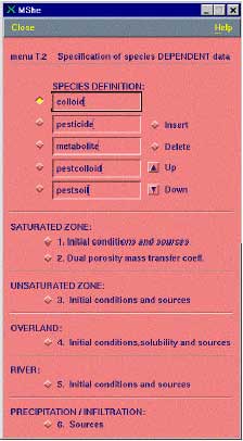
Figure 2.4 Input for MIKE SHE AD-module. This is only relevant if the module is used without the PestSurf interface
Figur 2.4. Input til MIKE SHEs AD-modul. Dette er kun relevant hvis modulet startes uden om PestSurf-brugerfladen
The species must be listed in the following order (see also Figure 2.4):
- colloid
- pesticide
- metabolite
- pestcolloid
- pestsoil (immobile)
- metcolloid
- metsoil (immobile)
Input for initial conditions, solubility and sources are given as usual, except that source-terms for colloids should be specified in the file 'setupname'.colloid. An example input file is shown in Figure 2.5. The meaning of the different input-parameters is explained below.
Figure 2.5 Example input file *.colloid
Figur 2.5 Eksempel på inputfil til kolloidberegningerne, *.colloid
Code for detachmentmodel: Refers to the three options for determing the detachment rates:
1: kinetic energy model
2: raindrop momentum model
3: MACRO-model
Waterdepth correction: exponential factor b in Equation (37)
Alpha: Coefficient (0≤α≤1), which determines the fraction of detached particles that infiltrate (See Equation (45)).
Parks/Rose/Eurosem: Determines which of the models to be used for calculating the water depth correction.
1: Parks
2: Rose
3: Eurosem
Soil type distrubution: Areal distribution of soil types. Can refer to .T2-file or be an integer number
No. of soil types: Number of different soil types in setup. Here two soil types are given, hence the soil data are repeated for each soil type.
Soil type code: Soil code used in the soil distribution file.
Detachability, Kd: Parameter Kd (T2L-2) in Equation (33). Erosion modelling gives a range of values from 2-10 kg/J for uncompacted soils and 8-44 kg/J for compacted soils (Morgan et al., 1998).
Soil resistance factor, A(e): Soil resistance factor A(e) (T2M-1L-3)in Equation (40) (Only relevant for detachment model 2)
Mulch factor, MA: Mulch factor MA (-) in Equation (40). (Only relevant for detachment model 2).
Replenishment rate, kr: Replenishment rate coefficient kr (M L-2 T-1) in Equation (46)
Dry bulk density, s: Dry bulk density of top soil s (ML-3) in Equation (46)
Influence depth, zi: Depth of top-soil influenced by detachment zi (L) in Equation (45)
Maximum detachable soil, Mmax: The maximum amount of detachable soil particles Mmax (g/s soil) in Equation (46)
Vegetation distribution: The distribution of vegetation in the model area is either specified with a single grid code value, if the same vegetation is present in the entire model area or by a .T2 map file containing a number of grid codes, each one representing a specific vegetation type. Each vegetation type is characterised by a number of different properties such as plant cover, plant height, angle and shape. The different plant properties are described in the following sections and must all be specified for each vegetation type.
No. of veg. types: The total number of plant types in the model is specified here. Here, two vegetation types are chosen and the vegetation data is repeated for each vegetation type.
Veg type code: The vegetation type code is an integer value representing a specific vegetation type, which is initially specified in the aforementioned map file.
Cover: The density of vegetation is expressed by the areal fraction of plant cover, which is dimensionless (0 < cover < 1). Can be given as a constant value or as a time series.
ICmax: ICmax is the maximum volume of interception by plant cover and is given as a water depth in [L]. Can be given as a constant value or as a time series.
Plant height: Effective plant height is used for computing the energy of leaf drainage in Equation (36) [L]. Can be given as a constant value or as a time series.
Plant angle: The plant angle is given in radii and is thus dimensionless.
Plant shape: Two different shapes of vegetation have been incorporated into the model. One type (1) represents grass or grass like vegetation and the other type (2) covers all other kinds of vegetation. The shape of the plants is of importance in computing stemflow. For grasses or vegetation with mean diameters smaller than the mean diameter of the drops, gravity plays an important role as opposed to other types of vegetation.
Canopy raindrop size: Canopy raindrop size is important in computing detachment by splash in relation to the computation of the water depth factor (L).
Stepmin: minimum time step used in the chemical solver
Stepmax: maximum time step used in the chemical solver
rtols: relative tolerance for the chemical solver
atols: absolute tolerance for the chemical solver
steps: the equilibrium reactions are solved as a set kinetic reactions with a forward and backward reaction. Steps specifies how much faster the slowest reaction rate for the equilibrium reactions is compared to the largest kinetic reaction rate. Large values will cause the equilibrium reactions to be more precisely described but could cause the solver to use smaller timesteps.
2.5 Transport and transmission process in the streams and ponds
The standard MIKE 11 AD (advection dispersion) module added on top of the standard MIKE 11 HD (hydrodynamic) module was used for description of the transport of active substances in the rivers caused by advection and dispersion. On top of the AD module a suite of process, which describes the sorption, biodegradation and other transport and transmissions process, was implemented in a dedicated MIKE 11 PE (pesticide) module. The following section gives a technical description of the process implemented in the pesticide module. A conceptual diagram of the process descriptions of the pesticide module appears from Figure 2.6.
Figure 2.6 Conceptual drawing of the MIKE 11 pesticide module
Figur 2.6 Konceptuel model af MIKE 11's pesticidmodul
2.5.1 Sedimentation and resuspension
processes for description of sedimentation and resuspension are implemented in the MIKE 11 pesticide module, but it was decided to set the exchange of sorbed active substances between the water column and the sediment to 0. For a further discussions thereof see Section 2.9 in Styczen et al. (2003a). Consequently a detailed description of the sedimentation and resuspension is not provided in the present report.
2.5.2 Diffusive exchange between water column and sediment in the rivers
In the river the sediment is supposed to be well mixed and a one-layer model of the sediment is therefore considered as appropriate. Under these assumption the diffusion from the water column in to the sediment is described by the following differential equations:
dCW/dt = D*AREA*(SW-CW)/(FZ*Volume),
(Eq. 49)
where
CW denotes the concentration of dissolved active substance in the water column
SW denotes the concentration of active substance in the pore water
FZ denotes the thickness of the laminar boundary layer
AREA denotes the area of the bottom
FZ denotes the thickness of the laminar boundary layer
D denotes the molecular diffusion coefficient
Volume denotes the volume of the water column
The diffusion from the pore water in to the water column is described by the following differential equation:
dSW/dt= D*AREA*(CW- SW)/(FZ*Volume),
(Eq. 50)
where
Volume denotes the volume of the pore water.
2.5.3 Diffusive exchange between water column and sediment in ponds
The sediment in the ponds is not assumed to be well mixed and diffusive process might therefore take place within the sediment. This diffusion, and the sorption and biodegradation of active substance is described by a module implemented in the AD scheme of the MIKE 11 model. A description and a testing of this module appear from Appendix E.
2.5.4 Sorption to particles in water column and sediment
Considering sorption as a reversible process the adsorption and desorption might be described as two opposite first order process (Nyffeler et al 1984) yielding the following differential equations:
dCW/dt = K2*CS - CW*K1
(Eq. 51)
and
dCS/dt = CW*K1 - K2*CS,
(Eq. 52)
where
CW denotes the concentration of active substance dissolved in water
CS denotes the concentration of active substance sorbed to particles
K1 denotes a (pseudo) first order adsorption rate
K2 denotes a first order desorption rate
The adsorption rate is in fact a pseudo first order rate constant, as described in experiment by Nyfeller et al. (1986) and expresses a linear relationship to the concentration of sorbing particles.
Or expressed mathematically:
K1 = K1**CP,
(Eq. 53)
where
K1* denotes the adsorption rate constant
CP denotes the concentration of particles in the water column or for the sediment the ratio between solid matter and water.
2.5.5 Sorption to macrophytes
The active substance in the water column might also sorb to macrophytes. As for the sorption to sediment particles and suspended matter the sorption to macrophytes was described by a first order sorption and a first order desorption rate. Hence the same basic equation as for sorption of active substances to particles was used except that the concentration of particles, CP, was substituted with the concentration of macrophytes.
2.5.6 Biodegradation of active substances
Dissolved active substances in the pore water and water column are assumed to undergo biodegradation. In every case the degradation will be formulated as a first order degradation yielding the differential Equations (54) and (55) for degradation of dissolved active substances in water and pore water respectively.
dCW/dt = Kcs*CW,
(Eq. 54)
where
CW denotes the concentration of dissolved active substance in the water column (g-pesticide/m3)
Kcw denotes a first order degradation rate for active substance dissolved in the water column(h-1)
dSW/dt = KsW*SW,
(Eq. 55)
where
SW denotes the concentration of active substance dissolved in the pore water (g-pesticide/m3)
KsW denotes a first order degradation rate for active substance dissolved in the pore water (h-1)
Biodegradation is influenced by temperature, where the rate increases with increasing temperature (Dickson et al, 1984). The temperature effect is usually presented by the Arrhenius-like Equation (57) as:
![]() ,
,
(Eq. 56)
where
T= water temperature (C)
To= reference temperature for which reaction rate is reported (C)
A = constant
At temperatures below 5°C, biodegradation is assumed to stop.
2.5.7 Photolytic degradation of active substances
As described in Section 2.14 of the calibration report (Styczen, 2004a) only the direct photolysis is accounted for by the MIKE 11 PE module. To calculate the photolytic degradation one needs to know the quantum yield defined as:
Click here to see the Equation.
Assuming that the amount of light absorbed by the chemicals is much less than the amount of light absorbed by the water body the light absorption of the compound per unit volume can be expressed as:
(Eq. 58)
where
Ia(λ) denotes the total number of quanta absorbed of the array of wavelength (λ)
W(λ) denotes the total light intensity at the surface distributed at the array of wavelength (λ)
ε(λ) denotes the decadic molar extinction coefficients distributed at the array of wavelength (λ) (mol quant m-1)
αD (λ) denotes the apparent or diffuse attenuation coefficients of river water distributed at the array of wavelength (λ)
Cd denotes the concentration of active substance
Depth denotes the depth of the river
Zmix depth of pond or river
α(λ) denotes the attenuation coefficients of river water distributed at the array of wavelength (λ)
When the total number of quanta absorbed, Ia(λ), and the reaction quantum yield, φr(λ), are known then a first order photolytic degradation rate, Kphoto, can be calculated as:
Kphoto = Ia(λ)*φr(λ),
(Eq. 59)
And the photolytic degradation can then be expressed by the differential equation:
dCW/dt = -Kphoto*CW,
(Eq. 60)
Generally, organic compounds including active substances should absorb light in the wavelength range of 290-600 nm in order to be photolytically transformed (Guenzi et al., 1974) and the light absorption spectra, ε(λ), for the active substance in this interval is available from the user interface. In addition is the reaction quantum yield φr(λ) (Schwarzenbach 1993) available from the user interface. On the contrary the remaining terms of Equation (6) have to be estimated on the basis of data from the catchments. Hence the attenuation coefficient, α(λ) have been set to 2.5 for all wavelength after the calibration exercise (Styczen et al 2004).
αD=α(λ)* D
(Eq. 61)
The diffuse or apparent attenuation coefficient is estimated on the basis of, α(λ), D(λ) and the equation of Neely and Blau (1985):
αD(λ) = α(λ)*D(λ),
(Eq. 62)
where
D(λ) denotes the ratio between the average path length and the depth for an array of wavelength (λ)
For both rivers D(λ) was set to 1.6 based on considerations of Neeley and Blau (1985), who stated that D(λ) is between 1.05 and 1.3 for blue and UV light in surface water and Schwarzenbach (1993), who stated that D() might be 2 in very turbid water. All though Equation (63) shows that the attenuation is a function of the wavelength it was assumed that α(λ) and αD(λ) is the same for all wavelengths (λ). This assumption was needed since the detailed chemical composition of the organic matter in the water not is known and the attenuation at different wavelength can therefore not be estimated.
2.5.8 Hydrolysis
The hydrolysis of organic chemicals in water is often observed as a first-order reaction given by (Thomann and Muller, 1987):
(Eq. 63)
where
KHT denotes the hydrolysis rate constant (h-1)
The hydrolysis rate constant (KHT) may include contributions from acid- and base-catalysed hydrolysis as well as nucleophilic attack by water (neutral hydrolysis). The following equation explains these possibilities explicitly:
![]()
(Eq. 64)
where:
KH denotes the acid catalysed hydrolysis rate constant (mol-1*h-1)
KOH denotes the base catalysed hydrolysis rates constant (mol-1*h-1)
KH2O denotes the neutral hydrolysis rates constant (h-1)
The acid, base and neutral hydrolysis constants are available from the user interface. [H+] and [OH-] was set to 7.5 and 6.5 respectively corresponding to the average measurements of pH conducted by the counties.
2.5.9 Evaporation
The evaporation of active substance from the water to the air is described by the same basic equation as for dry deposition outlined in Section 2.3.2. However, the MIKE 11 pesticide module calculates the evaporation for every time step of 3 minutes, whereas the model for dry deposition, PESTDEP, calculates the dry deposition to the river with a time resolution of one week. Due to the large differences in time resolution it is not relevant to link the two models dynamic. In the model the evaporation of active substances was therefore considered as independent from the dry deposition. As a consequence the concentrations of active substances in the air was set to 0 when the evaporation of active substances was calculated.
3 User Interface
The user interface is a bridge between the user and the scenarios. It transforms the parameters specified in its menus to time series, maps and files that are used to run the model. Each menu page is described in the following, and this is followed by a description of the transformations taking place between the user interface and the model.
3.1 How to start the system
Start the Mike Zero shell, press File, New, and select MIKE SHE/Pesticide in Surface water, or select File, Open and the appropriate parameter file (*.psw), if a file already exists.
Figure 3.1 Opening a file in PestSurf.
Figur 3.1 Åbning af fil i PestSurf.
3.2 The system
The model system allows the user to simulate active substance (and one metabolite) on six different scenairos, that is
- Lillebæk stream
- Lillebæk macorphyte dominated pond
- Lillebæk phytoplankton dominated pond
- Odder Bæk stream
- Odder Bæk macorphyte dominated pond
- Odder Bæk phytoplankton dominated pond
For each of the scenarios, a set of water movement files exists for each crop allowed in the user interface (14 crops in total, 13 water files per scenario as spring barley and spring wheat utilizes the same file). The files are named "Catchment"_"waterbody"_crop, with an extension that specifies whether it is a MIKE SHE or a MIKE 11-flow-file. These files are stored on external disks due to their size. The right disk has to be selected for the particular run. The selected water movement file is the basis for the calculation of solute transport. The directories, where the files are l°Cated, are selected via "Settings", see Figure 3.2.

Figure 3.2 Setting of the location of MIKE SHE Water Movement files.
Figur 3.2 Specifikation af placeringen af MIKE SHE's vandberegningsfiler.
In order to carry out the solute calculations, input parameters have to be specified for wind drift (see Section 2.1), for the dry deposition model "PestDep" (see Section 2.3), and the MIKE SHE and MIKE 11 solute transport and transformation modules. The menus described in Section 3.3 are used for specifying the necessary parameters. All other parameters are pre-specified in templates, which are stored separately in the system.
The basic input files required for MIKE SHE and MIKE 11 are shown in Table 3.1. Templates for all the necessary files are prepared and stored in the system. There are eight of each file, as they exist for each scenario and with and without Metabolite. For each catchment the templates for the macrophyte and phytoplankton dominated ponds are identical.
Table 3.1 File types and short description of files required for MIKE SHE and MIKE 11 active substance calculations.
Tabel 3.1 Filtype og kort beskrivelse af filer til MIKE SHE og MIKE 11-pesticidsimuleringer.
| MIKSHE | |
| .tsf –files | General solute transport parameters |
| .xtsf-files | Specific sorption and degradation parameters |
| MIKE 11 | |
| .bnd11 | Boundaries and sources for matter and water |
| .ad11 | Parameters for advection and dispersion |
| .pe11 | Parameters for transport and transmission of active substances |
| pesticide_diffusion.txt | Parameters for diffusion, adsorption and decay of active substances in the sediment beds of the ponds. |
| .sim11 | Specification of files for boundaries, sources and parameters |
The name-convention for the files is "Catchment"_"waterbody"_Pest/PestMetab.extension.
Some of the values in the above files are given standard values. One of each template file for MIKE SHE is included in Appendix B, and one of each template file for MIKE 11 is included in Appendix C, with comments on the selected standard values. The standard values selected for the colloid module is included in Appendix B.
When the menu-pages, described in Section 3.3, are filled out, and before the simulations can start, the input given on the menu-pages are transformed to the values required for the models to operate. This is done by a pre-processing programme.
The pre-processing programme:
- selects the correct water movement file
- selects the correct template files for MIKE 11 and MIKE SHE
- Calculates wind drift for each section of the stream or the water body (Section 2.1)
- Calculates dry deposition for each section of the stream or the waterbody (Section 2.3)
- Transforms the values for drift and dry deposition into time series files for MIKE 11
- Calculates a time series files for calculation of photolysis rate in MIKE 11 on the basis of the daily global radiation and the absorption spectra of the active substance
- Corrects the dose on the agricultural land according to the calculated drift and deposition losses (Section 2.2)
- Recalculates input values in the appropriate form and modifies the template files for MIKE SHE/MIKE 11 with the revised values.
- Creates a new directory with the name of the run and stores a copy of all the modified templates and other produced files.
The directory is divided into MAPS, MIKE11, TIME, SIGNALS and temp. The user can therefore always check the actual input used. When the user has finished working with a simulation, the whole directory can be removed without damaging the programme. However, the user may wish to store the parameter file (.psw) and the MIKE 11 Result file that includes the results to be displayed in the result presentation programme, se Section 4.
Table 3.2 List of files moved to the working directory established by the User interface when a simulation is initiated. Some of these are generated by the programme.
Tabel 3.2 Filer, der flyttes til arbejdsfolderen, der genereres af brugerfladen når simuleringen starter. Nogle af filerne genereres af programmet.
| location | File Name | Explanation |
| Under main directory | InputDryDepositionCalculations.txt | All input for the dry deposition calculation |
| . colloid | Input to colloid calculations | |
| .tsf | Input to MIKE SHE Advection-Dispersion module | |
| .xtsf | Input to MIKE SHE sorption/degradation module | |
| Spraying.psf | Input to winddrift and selected input to dry deposition calculations | |
| W5.* | Results from the last calculation of the dry deposition programme. | |
| \MAPS | Kd | Calculated values of Kd |
| DT50 | Calculated values of half life | |
| Agrl | Map indicating area to be sprayed. | |
| Rhob | Bulk density files used | |
| \MIKE11 | RES11-files | The selected water movement files (with the name of the catchment and the
crop are moved to this directory.
The RES11-file with the name of the directory is the output file of the scenario. |
| Hd11, xns11 and nwk | Describes the basic river system and stream setup. | |
| Ad11 | Parameters for the advection/dispersion simulation of MIKE11 | |
| Bnd11 | Specification of boundary conditions for MIKE11 | |
| Pe11 | Specification of Pesticide parameters for MIKE11 | |
| Sim11 | Specification of the overall simulation with MIKE 11 | |
| Pesticide_update_frequency.txt | The file is generated by the user interface and guides the frequency of storing of MIKE 11-results 1. | |
| Pesticide_diffusion.txt | Specification of pesticide parameters for the sediment in ponds | |
| \TIME | CropCover.T0 | Input to colloid programme |
| CropHeight.T0 | Input to colloid programme | |
| Crop Interception.T0 | Input to colloid programme | |
| SoilDeposit.dfs0 | Specifies the fraction of the pesticide depositing on the ground as a function of date. | |
| Deposition_stream_spray.dfs0 | Time series specifying the additions from spray drift and dry deposition on the different segments of the stream or pond | |
| _RiverDepth.dfs0 | Time series of variation in water body depth | |
| RiverWidth.dfs0 | Time series of variation in water body width | |
| Streamtemperature.dfs0 | Time series containing the temperature of the water body | |
| _prec.T0 | Time series of the precipitation | |
| _trd.T0 | Time seris of the air temperature | |
| Photolysis.dfs0 | Timeseries calculated on the basis of the light absorption spectra of the compound, the spectral composition of the sunlight and the daily global radiation. The timeserie is used for calculation of photolysis. | |
| Spraying_corr.T0 | The dosage sprayed on the fields (MIKE SHE) | |
| biomass.dfs0 | Timeseries of the biomass of macrophytes in ponds and streams. | |
| \SIGNALS | Contains log-files and error-messages from MIKE SHE, generated during the run | |
| \tmp | Temporary files of no interest. |
In addition to the above files, a number of support-files are used, either to specify particular parts of the setup, to re-calculate values to the right units or to distribute parameters in space. These files are listed in Table 3.3.
Table 3.3 Files that are used to transform menu-given parameters to distributed parameters in the catchments or waterbodies. The name convension is
Catchment_waterbody_Item_layernumber.T2 for maps.
Table 3.3 Filer, der bruges til at transformere værdier fra menuerne til distribuerede parametre i oplandet eller i å/vandhul. Navnekonvensionen er
Opland_vandtype_type_lagnummer.T2 for kort.
| Item | Explanation |
| F°C | Organic matter content in each layer of soil. For Lillebæk, this adds up to 11 maps, and for Odder Bæk to 7 maps for each scenario. |
| Fclay | Clay content in each layer of soil. For Lillebæk, this adds up to 11 maps, and for Odder Bæk to 7 maps for each scenario. |
| Moistcorr_pF2_ | Moisture and depth-correction fact at pF2. For Lillebæk, this adds up to 7 maps and for Odder Bæk to 5 maps for each scenario. |
| Moistcorr_pF1_ | Moisture and depth-correction fact at pF1. For Lillebæk, this adds up to 7 maps and for Odder Bæk to 5 maps for each scenario. |
The distribution of soil factors is based on the soil maps of the catchment, and the area to be sprayed on the presence of agricultural land in the catchments (Styczen et al., 2003a). The values for each soil profile and horizon are shown in Appendix D. The variables of organic matter and clay contents of the sediment and suspended matter were specific for each scenario and appear from Appendix E.
3.3 General Menu-pages
The menu pages are divided into three parts. To the left is a list of all the menu pages in the system, allowing the user to navigate through the pages. The system shows only the pages of relevance. If, for example, metabolites are not included in the simulations, the pages of relevance for metabolites disappear from the list.
To the right is the window where values have to be added. In the bottom of the menu is a field, where comments to input may occur. If the user forgets to enter a value, or a value is outside given limits, this will be registered here.
The help function is activated by F1 and it is context-sensitive.
3.3.1 Basic parameters
Figure 3.3 shows the first menu-page of the system. The user chooses whether or not to include a metabolite in the simulation. The active substance and metabolite names have to be specified. This choice influences the selection of template- and support-files for the setup of the model.
Figure 3.3 Menu page: Basic Parameters.
Figur 3.3 Menu-side: Basale parametre.
Initially, it was intended that the user interface should allow automatic selection of Monte Carlo parameters. This function has been not been implemented and is therefore not active. As the stream runs take about 24 hours, the time required to run a distribution of parameters is considerable.
3.3.2 Catchment and type of surface water
In the second menu (Figure 3.4), the scenario is selected. This includes
- the location (Lillebæk/Odder bæk), which is actually an expression of the type of landscape represented, Lillebæk being moraine and Odder Bæk representing more sandy conditions,
- the type of water body (stream/pond) and
- whether the pond is aerobic (macrophyte-dominated) or anaerobic (phytoplankton-dominated).
With the second menu completed, all the required files of Table 3.1, and the four file types of Table 3.3 are defined.
Figure 3.4 Menu-page: Catchment and type of surface water.
Figur 3.4 Menu-side: Opland og type af overfladevand.
3.3.3 Crop
The third menu (Figure 3.5) allows the user to choose the crop to be sprayed, and to set a transpiration factor for the active substance. The transpiration factor is a factor that defines the plant uptake of pesticide. The value may vary between 0 and 1, and is multiplied onto the concentration of the water taken up. In test runs it was noted that for spring applications, particularly in the moraine catchment, the model is very sensitive to this value, as a considerable part of the pesticide is taken up by plants, even with a transpiration factor of 0.4.
For spruce trees, the choice also concerns the age of the culture and whether it is sprayed horizontally. The reasoning for these choices are described in Section 2.1 and 2.2, but in short, the coverage percentages and the function used to calculate wind drift differ depending on plant age and spraying method.
With the selection of crop, the selection of water movement file is finalised. The choice also determines the type of wind drift formula to use.
Figure 3.5 Menu-page: Choice of crop. Spring wheat and spring barley uses the same pre-calculated water file.
Figur 3.5 Menu-side: Valg af afgrøde. Vårhvede og vårbyg bruger de samme for-beregnede vandfiler.
3.3.4 Width of protection zone
The next menu allows the user to select the width of the buffer zone. The choice influence the calculation of wind drift (Section 2.1), the calculation of dry deposition (Section 2.3.2) and the choice of file describing the size of agricultural land. As the grid size of the model is 50 m, the area to be sprayed cannot be successively reduced. If the buffer zone is greater than 35 m, the row of grids closest to the stream on both sides is removed from the sprayed area. The choice thus influence the selection of file specifying the sprayed area, the agrl_0 or agrl_35-file mentioned in Table 3.3.
Figure 3.6 Menu-page: Width of protection zone.
Figur 3.6 Menu-side: Bredde af bufferzonen.
3.3.5 Spraying data
The specification of the spraying data requires a dose and a date. To take into account the effect of date of spraying, the model should be run several times, with different possible spraying days selected in the relevant period of spraying. If, for example, the spraying period is 1st to 20th of May, the model could be run 4 times, e.g. on 1st, 6th, 11th, and 16th of May 2. This pr°Cedure is also used for the Danish grounDwater scenarios. The user can choose to allow or not allow spraying when rain occurs. If the user do not allow this, the spraying date is moved forward by eight hours until a period with no rain is encountered. As four different years are simulated, it is found somewhat artificial to find dates that in all years will fulfill particular criteria – this will allow very few spraying dates during the year.
More sprayings are specified by clicking on the "extra line" bottom (top left), and a new dose and the number of days between the first and the second spraying can be specified.
The dose is input to the wind drift calculation, the calculation of dry deposition and the further calculation in the soil. The correction of the dose to the soil is already described in Section 2.2.
When the spray drift and dry deposition has been calculated, time series files are generated for each stretch of the river or for the pond, containing the deposition of active substance on the water body over time.
Figure 3.7 Menu-page: Spraying data.
Figur 3.7 Menu-side: Sprøjtedata.
3.3.6 Basic chemical and physical properties of the active substance (and metabolite)
This menu (Figire 3.8) exists both for the active substance and metabolite 3.
Figure 3.8 Basic chemical and physical properties.
Figur 3.8 Basale kemiske og fysiske egenskaber.
The Cas number is specified as a text string.
The basic chemical properties of an active substance (or a metabolite) that have to be specified are:
- the molar weight,
- the pKa, the Kow of the neutral compound,
- the water solubility of the neutral compound (mg/l), and
- the vapour pressure (kPa).
Henry's constant can be should preferably be specified, but if not, it is calculated as
Henry's constant =
(Eq. 65)
where mol weight (g/mol), the vapour pressure (kPa) and the water solubility stem from the interface,
Universal_gas_constant = 0.0821 l*atm/mol*k
Reference temperature = 293 K, and
the transformation factor is 9.85E-06 Pa/atm
The assumed reference conditions are 20ºC and 1 atm. If the active substance is an acid or a base, Kow is re-calculated to fit the pH-value of the scenarios. Otherwise the Kow-value is used directly in the calculations. The transformations are done in the following manner:
if the compound is neutral
Kow=Kow_1
if the compound is an acid
(Eq. 66)
if the compound is a base
(Eq. 67)
The dry deposition programme utilises the vapor pressure and Henry's constant. The pKa-value is used to modify the dose available for evaporation (InputDryDepositionCalculations.txt). For all scenarios pH was set to 7.6.
The solubility of the compound is used in MIKE SHE as a maximum concentration allowed for distributed pesticide (.tsf-file). This mainly influences the colloid transport processes.
All of these parameters are used for the MIKE 11-calculations (*.PE11-file)
3.3.7 Sorption of active substance in soil
With respect to sorption in the soil, the user may choose between a linear and a Freundlich isotherm.
The default value for the exponent of a Freundlich isotherm is 0.9. The Freundlich isotherm is defined as x = Kfcref(c/cref)1/n, where x is the content of active substance sorbed (mg/kg), and c is the concentration in the liquid phase (mg/l). cref is the reference concentration, which is usually 1 mg/l. K must be given in dm3/kg (or l/kg).
Figure 3.9 Menu-page: Sorption of active substance in soil.
Figur 3.9 Menuside: Sorption af pesticid i jord.
It is important to note that if the Freundlich isotherm is used, the value of Kf is very sensitive to the units. In MIKE SHE, the internal calculations are in g/l and a transformation is therefore carried out as part of the pre-processing programme for sorption values used for Freundlich sorption:
![]()
(Eq. 68)
where
N = 1/n
K = Kf in mg/l
The sorption coefficient can be defined as a function of organic matter (KOM), as a function of organic carbon (KOC), as a function of clay (Kclay) or as a Kd-value of the soil. As % OC = % OM/1.724, KOC = KOM * 1.724. If KOC, KOM or Kclay is given, the sorption of each horizon in each soil profile is calculated as a function of the organic matter content or clay content of the respective horizon.
The equivalent Kd-value is the Kx * the fraction of the 'x' constituent of the soil. Maps of each of these constituents have been prepared (Table 3.3). The result of the pre-processing is therefore a series of maps (T2-files) of Kd-values that are referred to in the xtsf-file.
If nothing else is known, the user can estimate sorption from KOW in the following manner: log10(KOC) = 1.029*log10(KOW) – 0.18.
The value can also be used as input to the calculation of Kd for the MIKE 11 model of rivers and ponds, (see Section 3.3.9). To avoid an extrapolation to active substances concentrations far below the concentrations at which the empirical Freundlich equation was derived, linear sorption is always assumed for the streams and ponds.
A similar page should be filled out for the metabolite, if a metabolite is included in the calculation.
3.3.8 Degradation of active substance in soil
The menu allows specification of a degradation half life in days at 20 °C and at a moisture content equal to of either pF1 or pF2. The user also specifies a relative change in degradation rate with depth. The default values given are 1 from 0-30 cm's depth, 0.5 from 30-60 cm depth and 0.3 from 60 cm to 1 m. Note, that these values are corrections of the rate, and the DT50-value is thus inversely related to this factor.
Figure 3.10 Menu-page: Degradation of active substance in soil.
Figur 3.10 Menu-side: Nedbrydning af pesticid i jord.
It is possible to specify a Q10 value, this is the relative change in reaction velocity by a change in temperature of 10 degrees. The default value is 2.2 (FOCUS, 1996).
As the internal reference moisture content in MIKE SHE for degradation is the moisture content at saturation, the DT50 at pF1 or pF2 is re-calculated to DT50 at saturation. The formula used is:
![]()
(Eq. 69)
As this correction factor depends on the soil type, the correction factors are prepared as maps for different soil depths (see Table 3.3). The DT50 values are then corrected with the changes in degradation rate with depth (the inverse value is used on the DT50 as DT50 and degradation rate is inversely related). The result is a series of T2-maps of the DT50-values, referred to in the xtsf-input file.
The defined layers in Lillebæk and Odder Bæk follows horizons and discretisation. These layers are slightly different from the standard depths given for depth correction factors. Table 3.4 shows how the correction factors are used on the different layers in the two catchments.
Table 3.4 Utilisation of (default) depth correction factors on the layers defined for the Lillebæk and Odder Bæk-scenario.
Tabel 3.4 Anvendelse af (standard) dybdekorrektionsfaktorer for lagene defineret i Lillebæk-og Odder Bæk scenariet.
| Lillebæk | Odder Bæk | ||
| Depth, cm | Depth correction factor | Depth, cm | Depth correction factor |
| 0-30 | 1 | 0-25 | 1 |
| 30-40 | 0.5 | 25-35 | (1+0.5)/2 |
| 40-45 | 0.5 | 35-60 | 0.5 |
| 45-50 | 0.5 | 60-80 | 0.3 |
| 50-70 | (0.5+0.3)/2 | 80-100 | 0.3 |
| 70-80 | 0.3 | 100-150 | 0 |
| 80-100 | 0.3 | > 150 | 0 |
| 100-105 | 0* | ||
| 105-120 | 0 | ||
| 120-170 | 0 | ||
| >170 | 0 |
- As DT50-values are specified, and the rate is specified as the inverse value, a zero equals an infinitely large DT50-value. However, the model interprets a "0" as "no degradation".
In the model, the reference degradation rate is calculated as μ ref = ln2/(half life). The degradation rate is then modified according to temperature and moisture content according to the following formulas:
μ = μ ref* Fw*Ft, where
Ft = e α(T-Tref)
α= (lnQ10)/10 (for Q10 = 2.2,α = 0.079 K-1)
Fw = (θ /θ b)0.7
A similar page should be filled out for the metabolite, if a metabolite is included in the calculation.
The final maps produced are stored under \MAPS and referred to in the .xtsf-file.
3.3.9 Sorption of active substance in surface water
The menu page "Sorption of active substance in surface water" allows the user to choose between the use of the KOC, KOM, Kclay from soil or whether to calculate a value from Kow. If the user choose to calculate the Kd value from the sorption data given for the soil (Section 3.3.7) the following pr°Cedures are applied:
Figure 3.11 Menu-page: Sorption of active substance in surface water.
Figur 3.11 Menu-side: Sorption af pesticid i overfladevand.
If the input is KOC
Kd_Water = Kd_sediment = (KOC*LOI_Scen*1.724/ 1*106), where
LOI_Scen =Loss of ignition, weight % for the specific scenario.
If the input is Kom
Kd_Water = Kd_sediment = (Kom*LOI_Scen)/1*106, where
LOI_SCEN =Loss of ignition, weight% for the specific scenario.
If the input is Kclay
Kd_Water = Kd_sediment = (Kclay*(Clay_content))/1*106
where
Clay_content = Clay content for the specific scenario
The formulas used for calculation of Kd as a function of Kow are:
![]()
(Eq. 70)
where
Kow stems from the interface
LOI_Scen =Loss of ignition, weight % for the specific scenario
The loss of ignition values appear from Appendix F.
In addition the desorption rate is calculated from the following equation:
Desorption_Water = desorption_sediment = Sorption_rate/(Kd_Water*CP),
(Eq. 71)
where
Sorption_rate: 2.9
CP 83333 gm-3
To avoid an extrapolation to active substances concentrations far below the concentrations at which the empirical Freundlich equation was derived the Freundlich isoterm is always set to 1 when the sorption in the river was determined. Hence for the rivers linear sorption was assumed.
A similar page should be filled out for the metabolite 4, if a metabolite is included in the calculation.
The information is transferred to the .PE11-file.
3.3.10 Aerobic degradation of active substance in surface water
Figure 3.12 Menu-page: Aerobic degradation of active substance in surface water.
Figur 3.12 Menu-side: Aerobisk nedbrydning af pesticid i overfladevand.
A major aim of the sorption and biodegradation experiments of (Helweg et al 2003) was to develop an approach for estimation of the biodegradation of active substances in the sediment and in the water column. Ideally the approach should consider both the reduced bio-availability of the active substances in the sediment caused by sorption to particles and the relative differences in the bacterial activity in the sediment and the water column.
The approach is based on the following consideration:
From the user interface is a total biodegradation rate derived by the following equation:
(Eq. 72)
where T1/2 (days) is specified in the interface,
0.69 = ln(2),
24 is hours/day.
Or the total degradation of the active substance from the user interface might be described by the differential equation:
(Eq. 73)
where
CT denotes the total degradation of the active substance.
It is assumed that only dissolved active substances is degraded and that the degradation is attributable both to free living (pelagic) and to bacteria associated with particles. The activity of free living bacteria is assumed to be the same in the pore water and in the water column, whereas the activity of bacteria associated with particles is assumed to be proportional to the concentration of particles. Finally is it assumed that the degradation of active substances is proportional to the bacterial activity.
The degradation of the dissolved active substance might then be described by the following differential equation:
(Eq. 74)
where
(Eq. 75)
where
K1 denotes the relative activity of free living bacteria,
K2 denotes the relative activity of bacteria associated with particles,
K3 denotes a active substance specific degradation rate per bacterial activity,
Φ denotes the porosity of the suspension applied in the experiment.
Furthermore is it assumed that the bio-degradation rate is much lower than the sorption rate, which is supported by the sorption experiments of (Helweg et al 2003). If such the distribution of active substances between water and particles might be described by the following equation:
 , (mass active substance in water/total mass active substance)
(Eq. 76)
where
(Eq. 77)
where
ρs denotes mass density of the sediment particles
The relationship between the total concentration of active substance sorbed to particles and the concentration of dissolved active substance can then be written as:
![]()
(Eq. 78)
and (74), (75), (77) and (78) is combined to:
(Eq. 79)
and
(Eq. 80)
K2 and K1 are constants determined from the experiments of (Helweg et al 2003). The menu allows specification of a total degradation time for an experiment conducted at a given particle concentration.
The model requires specification of the bio-degradation in porewater, in the dissolved phase and on macrophytes. These values are derived from the total degradation as follows:
(Eq. 81)
where
T1/2 (days) is specified in the interface
0.69 = ln(2)
24 is hours/day.
![]()
(Eq. 82)
where
Φ is the porosity of the experiment of the user interface,
CP = the particle concentration of the experiment of the user interface (mg/l).
(Eq. 83)
where
fw = mass fraction of active substance in water and particles for the experiment of the user interface,
CP = the particle concentration of the experiment of the user interface (mg/l),
Kd values for the respective scenario determined from Section 3.3.9.
(Eq. 84)
where
K3 a active substance specific degradation constant,
CP the particle concentration of the experiment of the user interface (mg/l),
K1 a constant derived from the biodegradation experiments of (Helweg et al 2003),
K2 a constant derived from the biodegradation experiments of sub-project 5 (Helweg et al 2003).
Thereafter the degradation rates is calculated in the following way:
(Eq. 85)
![]()
(Eq. 86)
where
K4 Is a constant estimated on the basis of the calibration exircise for the pond models (Styczen et al 2004)
Values for K1, K2 and K4 appear from Appendix G.
The results are transferred to the PE11-file. A similar page should be filled out for the metabolite, if a metabolite is included in the calculation.
3.3.11 Anaerobic degradation of active substance in surface water
Anaerobic biodegradation is applied for the degradation of dissolved active substance in the pore water of the sediment in the phytoplankton dominated pond. The influence of particle concentration, or porosity, is taken in to account as described in Section 3.3.10.
The menu-page is identical to aerobic degradation (Figure 3.12) A similar page should be filled out for the metabolite, if a metabolite is included in the calculation.
3.3.12 Hydrolysis of active substance in surface water
The model interface allows specification of a half life for acid, basic and neutral hydrolysis. When hydrolysis experiments conducted at different pH is available the different values is readily calculated using for instance an excel spreadsheet, solving three of the following equations with three unknowns:
Measured Rate = Kacid[H+] + Kneutral + Kbasic[OH-]
An example of such a spreadsheet will be delivered together with the final model.
These are re-calculated to rates as
![]()
(Eq. 87)
![]()
(Eq. 88)
(Eq. 89)
Figure 3.13 Menu-page: Hydrolysis of active substance in surface water
Figur 3.13 Menu-side: Hydrolyse af pesticid i overfladevand
A similar page should be filled out for the metabolite, if a metabolite is included in the calculation.
3.3.13 Photolysis of active substance in surface water
For description of photolysis the user is required to specify the absorption spectrum of the compound, and the quantum yield. The quantum yield specifies how many mol of active substance that is degraded by one mol of photons absorbed. In addition the spectral composition of the light in the summer season and a time series of the global radiation at the surface is used by the model, as mentioned in Table 3.2. The global radiation data was measured data for Hornum(st. nr. 20501), which was considered to be representative for normal Danish conditions. The global radiation data is given for every day in the periods used for the scenarios. The composition of the solar insulation was calculated from data given by OECD (1995). On the basis of these information the photolytic decay is calculated as described in Section 2.5.7.
Figure 3.14 Menu-page: Photolysis of active substance in surface water
Figur 3.14 Menu-side: Fotolyse af pesticid i overfladevand
A similar page should be filled out for the metabolite 5, if a metabolite is included in the calculation.
3.3.14 Pesticide transformations to metabolite
The transformation of active substance to metabolite is not a one to one process. First of all, the metabolite is smaller than the active substance, and secondly, only a fraction of the active substance (fprocess)turns into this particular metabolite. The difference in molar weight is taken care of by the pre-processing programme, as the molar weights are dealt with elsewhere. The factor that has to be specified is the fraction of active substances (in terms of mol) that turns into this particular metabolite.
The fraction is specified for different processes, as it is not certain that all processes have the same stochiometry.
fweight, process = fprocess * mol weightmetabolite/mol weightpesticide
The fraction is transferred to the xtsf-file and the pe11-file and is used to define the production of metabolite:
1 g of degraded active substance => fweight,process g of metabolite.
Figure 3.15 Menu-page: active substance transformation to metabolite
Figur 3.15 Menu-side: Pesticid'ets omdannelse til metabolit
4 Result Presentation
Simulation result can be presented in several ways. A special spreadsheet has been prepared that displays the information in the result files in a graphical form and as tables. To the user it appears as if the results are displayed in Excell spreadsheets. In addition, the results can be viewed in MIKE View as ordinary MIKE 11-result files.
It should be noted that the first year of the simulation runs are given their "right" name. Therefore, the analysed years of the Odder Bæk scenario simulation are 1998-2005, while they are 1994-2001 for the Lillebæk scenario simulation.
4.1 Water balances
Due to the fact that limitations on the size of the water movement files limited the number of items that could be stored in each run, special runs were conducted with the specific aim of storing water balance informations. Tables with water balances are presented in Appendix E in the scenario report (Styczen et al., 2003b).
4.2 Solute balances
It is rather complicated to extract the values required for a mass balance as different processes are handled by different models. However, the simplest way to get an overview is the following:
For Wind drift and Dry deposition:
Open the file "Deposition_stream_spray.dfs0" under \TIME in the working directory. The file contains the amounts of solute arriving in the stream in mg/m2/sek, for each river section, over the eight scenario years.
To calculate the dosage entering the river by wind drift, take the concentration specified for the first half hour after spraying, and multiply with length and width of the stream, as well as the period (30 min). The ponds are only one segment, and the dimensions of the ponds are shown in Table 4.1. For the stream, the actual width of each segment of the stream at the time of spraying has to be found in the file "Input"DryDepositionCalculation.txt, as dx water for the respective segment and time.
The dry deposition is calculated in a similar fasion, except that the duration of spraying is either 7 or 21 days.
Table 4.1 Dimensions of streams and ponds in the scenario, for drift and deposition calculations.
Tabel 4.1 Dimensioner for vandløb og vandhuller i scenarierne, anvendt til drift og depositions-beregninger.
| Length, m | Width, m | |||||
| Lillebæk pond | 15.8 m | 15.8 | ||||
| Odder Bæk pond | 20 | 20 | ||||
| Lillebæk stream | 1540 | 230 | 230 | 180 | 440 | |
| Odder Bæk stream | 320 | 1610 | 1170 | 410 | 440 | |
For other pathways to the stream, balances are available in the .tpf-file in the working directory.
Balances are stored at the end of the file, for each 360 days. The period can be changed in the .tsf-files in the template directory, but preferably not to less than 30 days =720 hours as the file becomes very large. The print in the tpf-file is shown in Figure 4.1.
The file contains the names of the species simulated, the period of the mass balance, and the transport from and to the different components. Overland to river and SZ (= saturated zone) to river, including direct grounDwater exchange and drain flow, are the two direct sources of solute from MIKE SHE to MIKE 11, in units of mg/m3 = g/l. "Sources to overland" is the total input of solute in mg to the sprayed area of the scenario. This area can be found in the spraying.psf-file at the top.
Additionally, balances can be retrieved for every 720 hours with the AD-retrieval programme of MIKE SHE (this frequency is also specified in the .tsf-files for the run).
Figure 4.1 Solute balance of the tpf-file.
Figur 4.1 Stofbalance i tpf-filen.
4.3 Graphical presentation of stream results
The programme "StreamConAna" was developed to facilitate creation of an overview for all the simulated data. An example of the graphics of the plot is shown in Figure 4.3.
The programme is started by opening the relevant excell template. These are found by pressing start, programs, DHI Software, Pesticides in Surface Water, Pesticide Tables and the relevant scenario. One template exists for each of the scenarios.
The spreadsheet is divided into several pages. The work starts by opening the setup-page, shown in Figure 4.2.
The MIKE 11 result file to be analysed has to be specified first. The river name should correspond to the selected template. The EUM type must be "concentration", and the species name is the name of the species specified in the user interface. If other simulation parameters are of interest, the names of these are written in the .AD11 file under \MIKE11 of the working directory. An example of such species could be:
[CompList]
DATA = 1,'Pesticide', 2, 0
DATA = 2,'Pesticide-Colloid', 2, 0
DATA = 3, 'Porewater conc.', 2, 0
DATA = 4, 'Adsorbed sediment', 2, 0
DATA = 5, 'Suspended matter', 2, 0
DATA = 6, 'Adsorbed macrophytes', 2, 0
DATA = 7, 'Sediment layer thickness', 6, 0
DATA = 8,'metabolite', 2, 0
DATA = 9,'metabolite-Colloid', 2, 0
DATA = 10, 'Porewater conc. metabolite', 2, 0
DATA = 11, 'Adsorbed sediment metabolite', 2, 0
EndSect // CompList
Figure 4.2 Setup page of the result presentation programme.
Figur 4.2 Opsætningsside for resultatpræsentationsprogrammet.
After these fields have been filled out, the file should be opened.
The locations (in m) specified in the spreadsheet are five locations for each stream scenario that represents selected points along the stream of particular interest. If "-1" is specified instead of a distance, the point is left out of the further analyses. The programme translates the distances specified to calculation cells and the corresponding time series in the result file (item in file). An item number must only occur once in the list.
Below the locations, a number of concentrations are specified (ng/l). These concentrations may be the detection level, or another minimum concentration of interest, and different toxicity indices of interest. When they have been specified, the button "build tables" should be activated.
On the following pages, the results are depicted for each concentration level specified.
The plot in the upper left corner show the length of the stream (y-axis), the time of simulation (x-axis) and the concentration of pesticide in the stream (colours). It thus integrates all the information generated by the simulation. For the stream plots, the variation along the stream is visible. For the ponds, only the upstream part of the graphics is of relevance. The ponds are allowed to spill over into a stream, and this part of the plot is not of relevance for the analysis.
In the lower left part of the graphics are shown time series for each of the locations specified on the setup page.
The plot in the upper right corner is an attempt to show how much of the stream is affected when a peak moves through the river system. When the concentration is higher than the detection level at the lower end of the depicted stream, the maximum concentration obtained during the last 24 hours is recorded for each calculation cell in the river. These values are depicted in the plot. It is thus possible to see how many events have been identified above a certain concentration and how long a stretch of the river has been affected by concentrations above a certain level during the event.
The plot at the lower right may either show the number of events with a max. concentration exceeding a certain value or the number of events with a duration longer than a certain value.
An event with respect to occurrence of pesticide or metabolite in the water body is defined as the period in which the concentration is above a specified value, e.g. a detection limit.
Below the graphics is a set of tables, one for each point specified along the stream (or pond), see Table 4.2. As the tables are produced in Excell, the results can be moved directly to reports, as required. The graphics can be exported as a bitmap by clicking on the right mouse-button when it is positioned on the graphics.
Figure 4.3 Example of graphics in the result presentation programme.
Figur 4.3 Eksempel på grafik i resultatpræsentationsprogrammet.
Table 4.2 Example of a table generated by the result presentation programme.
Tabel 4.2 Eksempel på tabel genereret af resultatpræsentationsprogrammet.
Figure 4.4 Example of test run on the Odder Bæk stream scenario, viewed in MIKE VIEW.
Figur 4.4 Eksempel på testsimulering af Odder Bæk-scenariet, set med MIKE VIEW.
The results can also be viewed in MIKE VIEW, the standard viewer of MIKE 11. It allows analysis of the time series in greater detail, longitudinal plots of the stream and concentration profiles that can be depicted in time by a video. Figure 4.4 shows an example of a MIKE VIEW result-presentation.
4.4 Sediment concentrations
As the time series for sediment concentrations are similar to the concentrations in the stream, they can be interpreted with the aid of the same tools. This is done by substituting the name of the pesticide on the setup-page with the name "Adsorbed sediment" or "Porewater conc.", depending on which value is of interest.
5 Statistical Functions Included
Statistical functions have not been implemented in the user interface, since the execution of one run last for about two days. Considering that the intelligent Monte Carlo simulation would demand about 25 runs a statistical evaluation of the model output was considered as unrealistic for practical purposes. However, a spread sheet deriving 25 sets of input parameters on the basis of the properties of the active substances and the framework for intelligent Monte Carlo analysis provided by (Styczen et al 2003) have been prepared. The spreadsheet consist of two input pages and an output page. The first input page is similar to the input page of the user interface. At the second input page the uncertainty of selected input parameters must be tabulated in terms of a standard deviation for the log transformed data. Hence it is assumed that the input parameters follows a log normal distribution. When the input pages have been filled out a suggestions for 25 data sets appear from the output menu. The data sets can then be entered to the user interface of the model and the output of these 25 model runs can be used for statistical evaluations.
6 References
Asman, W.A.H., Jørgensen, A. and Jensen, P.K. (2003): Dry deposition and spray drift of pesticides to nearby water bodies. - Ministry of Environment, Danish Environmental Protection Agency, Pesticides Research No. 66.
BBA (2000): Bekanntmachung des Verzeichnisses risikomindernder Anwendungsbedingungen für Nichtzielorganismen. Bundesanzeiger Nr. 100, 9879-9880, Germany, May 26, 2000.
Brandt, C. J., 1989. The size distribution of throughfall drops under vegetation canopies. Catena 16, pp. 507-524.
DHI (1997): MIKE 11 – User Guide
FOCUS Soil Group (1996): Soil Persistence Models and EU-Registration. European Commission Document 7617/VI/96.
Green, R.E. and KaricKHoff, S.W. (1990): Sorption estimates for modeling. In: Cheng, H.H. (ed): Pesticides in the soil environment: processes, impacts, and modeling. Soil Science Society of America Inc., Madison, Wisconsin, USA, 79-101.
Hairsine, P.B. and Rose,C.W. 1991. Rainfall Detachment and Deposition: Sediment Transport in the absence of Flow-Driven processes. Soil Sci. Soc. Am., Journal 55, pp. 320-324.
Helweg, C., Mogensen, B.B., Sørensen, P.B., Madsen, T., Rasmussen, D. and Petersen, S. (2003): Fate of pesticides in surface waters, Laboratory and Field Experiments. Ministry of Environment, Danish Environmental Protection Agency, Pesticides Research No. 68.
Holm, J., Petersen, C., KOCh, C. and Villholth, K.G. (2003): Facilitated transport of pesticides. - Ministry of Environment, Danish Environmental Protection Agency, Pesticides Research No. 67.
Iversen, H.L., Kronvang, B., Vejrup, K., Mogensen, B.B., Hansen, A.M. and Hansen, L.B. (2003): Pesticides in streams and subsurface drainage water within two arable catchments in Denmark: Pesticide application, concentration, transport and fate. - Ministry of Environment, Danish Environmental Protection Agency, Pesticides Research No. 69.
Jarvis, N, and Larsson, M. (1998): The MACRO Model (Version 4.1), Technical Description, SLU, Dep. of Soil Sciences, Uppsala.
Jensen, P.K. and Spliid, N.H. (2003): Deposition of pesticides on the soil surface. - Ministry of Environment, Danish Environmental Protection Agency, Pesticides Research No. 65.
Morgan, R.P.C., Quinton, J.N., Smith, R.E., Govers, G., Poesen, J.W.A., Auerswald, K., Chisci, G., Torri, D., Styczen, M.E. 1998c. The European Soil Erosion Model (EUROSEM): Documentation and user guide. Cranfield university, version 3.6.
Møhlenberg, F., Petersen, S., Gustavson, K., Lauridsen, T. and Friberg, N. (2001): Guidelines for evaluating meSocosm experiments in connection with the approval pr°Cedure. - Ministry of Environment and Energy, Danish Environmental Protection Agency, Pesticides Research No. 56.
OECD (1995) Direct phototransformation of chemicals in water. A draft guidance Document. February 1995.
Park, S.W., Mitchell, J.K. and Scarborough, J. N., 1982. Soil Erosion Simulation on Small Watersheds: A modified ANSWERS Model. Transactions of the ASAE, 25(6).
Refsgaard, J.C., Storm, B., 1995. MIKE SHE. In: Singh, V.P. (Ed). Computer Models of Watershed Hydrology, Water Resources Publication, pp.809-846.
Styczen, M., Petersen, S., Christensen, M., Jessen, O.Z., Rasmussen, D., Andersen, M.B. and Sørensen, P.B. (2004a): Calibration of models describing pesticide fate and transport in Lillebæk and Odder Bæk Catchment. - Ministry of Environment, Danish Environmental Protection Agency, Pesticides Research No. 62.
Styczen, M., Petersen, S. Sørensen, P.B., Thomsen, M and Patrik, F. (2004b): Scenarios and model describing fate and transport of pesticides in surface water for Danish conditions. - Ministry of Environment, Danish Environmental Protection Agency, Pesticides Research No. 63.
Styczen, M., Petersen, S., Olsen, N.K. and Andersen, M.B. (2004c): Technical Documentation of PestSurf, a model describing fate and transport of pesticides in surface water for Danish Conditions. - Ministry of Environment, Danish Environmental Protection Agency, Pesticides Research No. 64.
Appendix A
1 Measured and Fitted Wind Drift Curves
For agricultural crops:
| Distance | deposition, % of appl. Dose | ||
| m | measured | model | |
| 0 | 25.70 | ||
| 1 | 3.51 | 3.51 | |
| 2 | 1.24 | 1.23 | |
| 3 | 0.98 | 1.02 | |
| 4 | 0.94 | 0.90 | |
| 5 | 0.75 | 0.76 | |
| 7.5 | 0.42 | 0.44 | |
| 10 | 0.33 | 0.32 | |
| 15 | 0.2 | 0.19 | |
| 20 | 0.12 | 0.13 | |
| 30 | 0.11 | 0.11 | |
For apples:
| Distance | early stages | late stages | ||
| m | Measured | Model | Measured | Model |
| 1 | 34.3 | 23.0 | ||
| 2 | 30.3 | 18.9 | ||
| 3 | 29.6 | 26.6 | 15.5 | 15.5 |
| 4 | 23.5 | 12.8 | ||
| 5 | 19.5 | 20.7 | 10.1 | 10.5 |
| 7.5 | 14.1 | 15.0 | 6.4 | 6.4 |
| 10 | 10.6 | 11.0 | 4.4 | 4.1 |
| 15 | 6.2 | 6.7 | 2.5 | 2.5 |
| 20 | 4.2 | 4.0 | 1.4 | 1.5 |
| 30 | 2.0 | 1.5 | 0.6 | 0.6 |
| 40 | 0.4 | 0.5 | 0.2 | |
| 50 | 0.2 | 0.2 | 0.1 | |
For Spruce:
The final equation is the average of the fitted curves for early and late wine.
| Distance | late vines | early vines | ||
| m | measured | model | measured | model |
| 1.0 | 19.7 | 29.4 | ||
| 1.1 | 17.0 | 25.8 | ||
| 1.2 | 14.8 | 23.0 | ||
| 1.3 | 13.1 | 20.7 | ||
| 1.4 | 11.7 | 18.7 | ||
| 1.5 | 11.1 | 17.9 | ||
| 3.0 | 3.6 | 3.6 | 6.8 | 6.8 |
| 5.0 | 1.6 | 1.6 | 3.4 | 3.4 |
| 7.5 | 0.9 | 0.9 | 2.0 | 2.0 |
| 10.0 | 0.6 | 0.6 | 1.4 | 1.4 |
| 15.0 | 0.3 | 0.3 | 0.8 | 0.8 |
| 20.0 | 0.2 | 0.2 | 0.5 | 0.5 |
Appendix B
1 Tsf- and xtsf-file Samples
1.1 Sample tsf-file: Odderb�k_stream_PestMetab.tsf
Italicized sections are modified by the scenario-administrator of the user interface.
FILETYPE DATATYPE VERNO: 2001 1 521 =================================================== SETUP DATA for Transport Simulation =================================================== THIS FILE OK (T/F) : T =================================================== RESULTS OF WATERMOVEMENT CALCULATION Filename : Odderbaek_Stream_Apples.frf =================================================== SPECIES IN CALCULATION No. of species : 7 =================================================== SIMULATION CONTROL PARAMETERS ------------------- Simulation Identification Simulation title : Odderbaek Simulation descr : Integrated hydrological model for solute transport ------------------- Simulation period Cycle Option 1/2/3 : 2 Start year : 1998 Start month : 1 Start day : 2 Start hour : 0 Start minute : 0 End year : 2005 End month : 12 End day : 31 End hour : 0 End minute : 0 Cycle restart year : 1998 Cycle restart month: 1 Cycle restart day : 1 Cycle restart hour : 0 Cycle restart min : 0 Cycle end year : 2002 Cycle end month : 1 Cycle end day : 1 Cycle end hour : 0 Cycle end minute : 0 Stat. Flow year : Stat. Flow month : Stat. Flow day : Stat. Flow hour : Stat. Flow minute : ------------------- Execution Logicals Execute SZ T/F : F Execute All. T/F : T ------------------- Extensions SZ Double Por. : F ------------------- Inclusions of sources SZ T/F : F UZ T/F : F Overland T/F : T River T/F : F Prec./Inf. T/F : F ------------------- Storing of Results Storing SZ T/F: T Storing UZ T/F: T Storing OverlandT/F: T Storing River T/F: T Storing MBL r T/F: T St.Frq SZ : 2160.000000 St.Frq UZ : 2160.000000 St.Frq Overland : 2160.000000 St.Frq River : 2160.000000 St.Frq MassBal. : 2160.000000 Print frq MBL : 2160.000000 ------------------- Time Step Control Max SimTimeStep SZ : 2400.000000 Max SimTimeStep UZ : 2400.000000 Max SimTimeStep Ovl: 2400.000000 Max SimTimeStep Riv: 1000000000000.000000 Max Advec.Cour. SZ : 0.800000 Max Advec.Cour. UZ : 0.800000 Max Advec.Cour.Ovl : 0.800000 Max Advec.Cour.Riv : 0.800000 Max Disp.Cour. SZ : 0.600000 Max Disp.Cour. UZ : 0.600000 Max Disp.Cour. Ovl : 0.600000 Max Disp.Cour.Riv : 0.600000 Max Transport SZ : 0.900000 Max Transport UZ : 0.900000 Max Transport Overl: 0.900000 Max Transport River: 0.900000 =================================================== SZ INPUT PART ------------------- Effective porosity No of data elements: 1 Lower layer : 6 Porosity : 0.3 ------------------- Type of dispersion description Aniso. opt. 1/2/3 : 1 ------------------- Dispersivities No of data elements: 1 Lower Layer : 99 Disp. alfa LHH : 0.05 Disp. alfa THH : 0.05 Disp. alfa TVH : Disp. alfa LVV : Disp. alfa THV : ------------------- Matrix porosity No of data elements: 0 ------------------- Source locations No of data elements: 0 =================================================== UZ INPUT PART ------------------- Dispersivities No of data elements: 1 Depth : 99.000000 Dispersion : 0.050000 ------------------- Source locations No of data elements: 0 =================================================== OVERLAND INPUT PART ------------------- Dispersion X-disp. coeff. : 0.0 Y-disp. coeff. : 0.0 ------------------- Source locations No of data elements: 1 Location number : 1 Source type : 2 Area distribution : MAPS\Odderb�k_Stream_agrl0.T2 X coordinate : Y coordinate : =================================================== RIVER INPUT PART ------------------- River dispersion disp. coeff. : 0.050000 ------------------- Source locations No of data elements: 0 =================================================== PRECIPITATION/INFILTRATION INPUT PART ------------------- Source locations No of data elements: 0 ++*+*+*++*++*+*+*++*+*+*+*+*+**+*+*+*+*+*+*+*+*+*+*+*+*+*+*+*+*+*+*+* SPECIES DEPENDENT DATA ++*+*+*++*++*+*+*++*+*+*+*+*+**+*+*+*+*+*+*+*+*+*+*+*+*+*+*+*+*+*+*+* ------------------- Species Species name : Colloid =================================================== SZ INPUT PART ------------------- Initial Conditions No of data elements: 1 Lower layer : 99 Concentration : 0.0 ------------------- Source strength No of data elements: 0 ------------------- Dual Porosity Mass Transfer Coeff No of data elements: 0 =================================================== UZ INPUT PART ------------------- Initial conditions No of data elements: 1 Depth : 100.0 Concentration : 0.0 ------------------- Source strength No of data elements: 0 =================================================== OVERLAND INPUT PART ------------------- Initial Conc. and Solubility Initial Conditions : 0 Solubility : 1000.000000 ------------------- Source strength No of data elements: 0 =================================================== RIVER INPUT PART ------------------- Initial Conditions Initial conc. : 0.0 ------------------- Source Strength No of data elements: 0 =================================================== PRECIPITATION/INFILTRATION INPUT PART ------------------- Source strength No of data elements: 0 +*+*++*+*+*+*+*+*+*+*+*+*+*+*+*+*+*+*+*+*+*+*+*+*+* ------------------- Species Species name : Pesticide =================================================== SZ INPUT PART ------------------- Initial Conditions No of data elements: 1 Lower layer : 99 Concentration : 0 ------------------- Source strength No of data elements: 0 ------------------- Dual Porosity Mass Transfer Coeff No of data elements: 0 =================================================== UZ INPUT PART ------------------- Initial conditions No of data elements: 1 Depth : 99 Concentration : 0 ------------------- Source strength No of data elements: 0 =================================================== OVERLAND INPUT PART ------------------- Initial Conc. and Solubility Initial Conditions : 0 Solubility : 1000.000000 ------------------- Source strength No of data elements: 1 Location number : 1 Time series : TIME\spraying_corr.T0 Record number : 1 =================================================== RIVER INPUT PART ------------------- Initial Conditions Initial conc. : 0 ------------------- Source Strength No of data elements: 0 =================================================== PRECIPITATION/INFILTRATION INPUT PART ------------------- Source strength No of data elements: 0 +*+*++*+*+*+*+*+*+*+*+*+*+*+*+*+*+*+*+*+*+*+*+*+*+* +*+*++*+*+*+*+*+*+*+*+*+*+*+*+*+*+*+*+*+*+*+*+*+*+* ------------------- Species Species name : Metabolite =================================================== SZ INPUT PART ------------------- Initial Conditions No of data elements: 1 Lower layer : 99 Concentration : 0.0 ------------------- Source strength No of data elements: 0 ------------------- Dual Porosity Mass Transfer Coeff No of data elements: 0 =================================================== UZ INPUT PART ------------------- Initial conditions No of data elements: 1 Depth : 100.0 Concentration : 0.0 ------------------- Source strength No of data elements: 0 =================================================== OVERLAND INPUT PART ------------------- Initial Conc. and Solubility Initial Conditions : 0.0 Solubility : 1000.000000 ------------------- Source strength No of data elements: 0 =================================================== RIVER INPUT PART ------------------- Initial Conditions Initial conc. : ------------------- Source Strength No of data elements: 0 =================================================== PRECIPITATION/INFILTRATION INPUT PART ------------------- Source strength No of data elements: 1 Location number : 1 Time series : 0 Record number : 1 +*+*++*+*+*+*+*+*+*+*+*+*+*+*+*+*+*+*+*+*+*+*+*+*+* ------------------- Species Species name : Pestcolloid =================================================== SZ INPUT PART ------------------- Initial Conditions No of data elements: 1 Lower layer : 99 Concentration : 0.0 ------------------- Source strength No of data elements: 0 ------------------- Dual Porosity Mass Transfer Coeff No of data elements: 0 =================================================== UZ INPUT PART ------------------- Initial conditions No of data elements: 1 Depth : 100.0 Concentration : 0.0 ------------------- Source strength No of data elements: 0 =================================================== OVERLAND INPUT PART ------------------- Initial Conc. and Solubility Initial Conditions : 0.0 Solubility : 100000002004087730000.000000 ------------------- Source strength No of data elements: 0 =================================================== RIVER INPUT PART ------------------- Initial Conditions Initial conc. : ------------------- Source Strength No of data elements: 0 =================================================== PRECIPITATION/INFILTRATION INPUT PART ------------------- Source strength No of data elements: 1 Location number : 1 Time series : 0 Record number : 1 +*+*++*+*+*+*+*+*+*+*+*+*+*+*+*+*+*+*+*+*+*+*+*+*+* ------------------- Species Species name : Pestsoil =================================================== SZ INPUT PART ------------------- Initial Conditions No of data elements: 1 Lower layer : 99 Concentration : 0.0 ------------------- Source strength No of data elements: 0 ------------------- Dual Porosity Mass Transfer Coeff No of data elements: 0 =================================================== UZ INPUT PART ------------------- Initial conditions No of data elements: 1 Depth : 100.0 Concentration : 0.0 ------------------- Source strength No of data elements: 0 =================================================== OVERLAND INPUT PART ------------------- Initial Conc. and Solubility Initial Conditions : 0.0 Solubility : 0.000000 ------------------- Source strength No of data elements: 0 =================================================== RIVER INPUT PART ------------------- Initial Conditions Initial conc. : ------------------- Source Strength No of data elements: 0 =================================================== PRECIPITATION/INFILTRATION INPUT PART ------------------- Source strength No of data elements: 1 Location number : 1 Time series : 0 Record number : 1 +*+*++*+*+*+*+*+*+*+*+*+*+*+*+*+*+*+*+*+*+*+*+*+*+* ------------------- Species Species name : Metcolloid =================================================== SZ INPUT PART ------------------- Initial Conditions No of data elements: 1 Lower layer : 99 Concentration : 0.0 ------------------- Source strength No of data elements: 0 ------------------- Dual Porosity Mass Transfer Coeff No of data elements: 0 =================================================== UZ INPUT PART ------------------- Initial conditions No of data elements: 1 Depth : 100.0 Concentration : 0.0 ------------------- Source strength No of data elements: 0 =================================================== OVERLAND INPUT PART ------------------- Initial Conc. and Solubility Initial Conditions : 0.0 Solubility : 0.000000 ------------------- Source strength No of data elements: 0 =================================================== RIVER INPUT PART ------------------- Initial Conditions Initial conc. : ------------------- Source Strength No of data elements: 0 =================================================== PRECIPITATION/INFILTRATION INPUT PART ------------------- Source strength No of data elements: 0 +*+*++*+*+*+*+*+*+*+*+*+*+*+*+*+*+*+*+*+*+*+*+*+*+* ------------------- Species Species name : Metsoil =================================================== SZ INPUT PART ------------------- Initial Conditions No of data elements: 1 Lower layer : 99 Concentration : 0.0 ------------------- Source strength No of data elements: 0 ------------------- Dual Porosity Mass Transfer Coeff No of data elements: 0 =================================================== UZ INPUT PART ------------------- Initial conditions No of data elements: 1 Depth : 100.0 Concentration : 0.0 ------------------- Source strength No of data elements: 0 =================================================== OVERLAND INPUT PART ------------------- Initial Conc. and Solubility Initial Conditions : 0. Solubility : 0.000000 ------------------- Source strength No of data elements: 0 =================================================== RIVER INPUT PART ------------------- Initial Conditions Initial conc. : ------------------- Source Strength No of data elements: 0 =================================================== PRECIPITATION/INFILTRATION INPUT PART ------------------- Source strength No of data elements: 0 +*+*++*+*+*+*+*+*+*+*+*+*+*+*+*+*+*+*+*+*+*+*+*+*+* COLLOID : T EXTRA TSF FILE : T MIKE11 AD : T MIKE11 FILE NAME : MIKE11\Odderb�k_Stream_PestMetab.sim11 MIKE11 time step : 90 DISABLE VALIDATION OF HD RES FILE : T 1.2 Sample xtsf-file: Odderb�k_stream_PestMetab.xtsf Coloured sections are modified by the scenario-administrator of the user interface. FILETYPE DATATYPE VERNO: 2002 1 524 =================================================== EXTRA SETUP DATA for Transport Simulation =================================================== PROCESSES IN CALCULATION No. of processes : 12 =================================================== ------------------- Extensions Sorption : T Decay : T Soil temperature : T Plant uptake : T =================================================== FR INPUT PART ------------------- Air temperature Air temp grid codes: 1 Air temp tim.ser : TIME/Odderb�k_ted.T0 =================================================== SZ INPUT PART ------------------- Bulk density No of data elements: 1 Lower layer : 999 Bulk density : MAPS/Odderb�k_stream_rhob7.t2 ------------------- Initial soil temperature No of data elements: 1 Lower layer : 999 Init. soil temp. : 8. =================================================== UZ INPUT PART ------------------- Bulk density No of data elements: 7 depth : 0.25 Bulk density : MAPS/Odderb�k_stream_rhob1.t2 depth : 0.35 Bulk density : MAPS/Odderb�k_stream_rhob2.t2 depth : 0.60 Bulk density : MAPS/Odderb�k_stream_rhob3.t2 depth : 0.80 Bulk density : MAPS/Odderb�k_stream_rhob4.t2 depth : 1.00 Bulk density : MAPS/Odderb�k_stream_rhob5.t2 depth : 1.50 Bulk density : MAPS/Odderb�k_stream_rhob6.t2 depth : 99.0 Bulk density : MAPS/Odderb�k_stream_rhob7.t2 ------------------- Initial soil temperature No of data elements: 1 Depth : 999.0 Init. soil temp. : 8. ++*+*+*++*++*+*+*++*+*+*+*+*+**+*+*+*+*+*+*+*+*+*+*+*+*+*+*+*+*+*+*+* SPECIES DEPENDENT DATA ++*+*+*++*++*+*+*++*+*+*+*+*+**+*+*+*+*+*+*+*+*+*+*+*+*+*+*+*+*+*+*+* ------------------- Species Species name : Colloid =================================================== FR INPUT PART ------------------- Plant uptake transpiration factor transp.factor (0-1): 0.0 =================================================== UZ INPUT PART ------------------- Matrix-Macropore Mass Transfer Coeff No of data elements: 1 Depth : 999.0 Diffusion : 1.e-8 ++*+*+*++*++*+*+*++*+*+*+*+*+**+*+*+*+*+*+*+*+*+*+*+*+*+*+*+*+*+*+*+* ------------------- Species Species name : Pesticide =================================================== FR INPUT PART ------------------- Plant uptake transpiration factor transp.factor (0-1): 0.0 =================================================== UZ INPUT PART ------------------- Matrix-Macropore Mass Transfer Coeff No of data elements: 1 Depth : 999.0 Diffusion : 4.3e-5 FOCUS(2000) ++*+*+*++*++*+*+*++*+*+*+*+*+**+*+*+*+*+*+*+*+*+*+*+*+*+*+*+*+*+*+*+* ------------------- Species Species name : Metabolite =================================================== FR INPUT PART ------------------- Plant uptake transpiration factor transp.factor (0-1): 0.0 =================================================== UZ INPUT PART ------------------- Matrix-Macropore Mass Transfer Coeff No of data elements: 1 Depth : 999.0 Diffusion : 4.3e-5 FOCUS(2000) ++*+*+*++*++*+*+*++*+*+*+*+*+**+*+*+*+*+*+*+*+*+*+*+*+*+*+*+*+*+*+*+* ------------------- Species Species name : Pestcolloid =================================================== FR INPUT PART ------------------- Plant uptake transpiration factor transp.factor (0-1): 0.0 =================================================== UZ INPUT PART ------------------- Matrix-Macropore Mass Transfer Coeff No of data elements: 1 Depth : 999.0 Diffusion : 0.0 ++*+*+*++*++*+*+*++*+*+*+*+*+**+*+*+*+*+*+*+*+*+*+*+*+*+*+*+*+*+*+*+* ------------------- Species Species name : Metcolloid =================================================== FR INPUT PART ------------------- Plant uptake transpiration factor transp.factor (0-1): 0.0 =================================================== UZ INPUT PART ------------------- Matrix-Macropore Mass Transfer Coeff No of data elements: 1 Depth : 999.0 Diffusion : 0.0 ------------------- Species Species name : Pestsoil =================================================== FR INPUT PART ------------------- Plant uptake transpiration factor transp.factor (0-1): 0.0 =================================================== UZ INPUT PART ------------------- Matrix-Macropore Mass Transfer Coeff No of data elements: 1 Depth : 999.0 Diffusion : 1.e-8 ++*+*+*++*++*+*+*++*+*+*+*+*+**+*+*+*+*+*+*+*+*+*+*+*+*+*+*+*+*+*+*+* ------------------- Species Species name : Metsoil =================================================== FR INPUT PART ------------------- Plant uptake transpiration factor transp.factor (0-1): 0.0 =================================================== UZ INPUT PART ------------------- Matrix-Macropore Mass Transfer Coeff No of data elements: 1 Depth : 999.0 Diffusion : 1.e-8 ++*+*+*++*++*+*+*++*+*+*+*+*+**+*+*+*+*+*+*+*+*+*+*+*+*+*+*+*+*+*+*+* PROCESS DEPENDENT DATA ++*+*+*++*++*+*+*++*+*+*+*+*+**+*+*+*+*+*+*+*+*+*+*+*+*+*+*+*+*+*+*+* ------------------- Process identification Process name : (de)sorption of Pesticide on Colloid Proc. type 1/2/3/4 : 3 =================================================== GENERAL PROCESS PARAMETERS ------------------- Species definitions Dissolved species : Pesticide Sorbed species : Pestcolloid ------------------- Type of sorption description EQ/EQ+KIN 1/2 : 1 ------------------- Type of Equilibrium-sorption Lin/Freu/Lang 1/2/3: 1 ------------------- Type of Kinetic-sorption No Hyst./Hyst. 1/2 : 1 ------------------- Fracture sorption Bias factor (only for DP) Frac-sorp bias fac : 0. =================================================== SZ-RELATED PROCESS PARAMETERS ------------------- Sorption coefficients No of data elements: 1 Lower layer : 999 K1 (EQ) : 0.0 # 0 l/kg K2 (EQ) : 0. # exponent cN (N=1) K3 (KIN) : 0.0 # s-1 sorption rate K4 (KIN) (hyst.) : 0.0 # s-1 desorption =================================================== UZ-RELATED PROCESS PARAMETERS ------------------- Sorption coefficients No of data elements: 1 Depth : 99. K1 (EQ) : 0.0 K2 (EQ) : 0. K3 (KIN) : 0.0 K4 (KIN) (hyst.) : 0.0 ++*+*+*++*++*+*+*++*+*+*+*+*+**+*+*+*+*+*+*+*+*+*+*+*+*+*+*+*+*+*+*+* ------------------- Process identification Process name : (de)sorption of Pesticide on soil Proc. type 1/2/3/4 : 3 =================================================== GENERAL PROCESS PARAMETERS ------------------- Species definitions Dissolved species : Pesticide Sorbed species : Pestsoil ------------------- Type of sorption description EQ/EQ+KIN 1/2 : 1 ------------------- Type of Equilibrium-sorption Lin/Freu/Lang 1/2/3: 1 ------------------- Type of Kinetic-sorption No Hyst./Hyst. 1/2 : 1 ------------------- Fracture sorption Bias factor (only for DP) Frac-sorp bias fac : 0. =================================================== SZ-RELATED PROCESS PARAMETERS ------------------- Sorption coefficients No of data elements: 1 Lower layer : 999 K1 (EQ) : MAPS/Odderb�k_stream_pest_Kd7.t2 K2 (EQ) : 0.0 K3 (KIN) : 0.0 K4 (KIN) (hyst.) : 0.0 =================================================== UZ-RELATED PROCESS PARAMETERS ------------------- Sorption coefficients No of data elements: 7 Depth : 0.25 K1 (EQ) : MAPS/Odderb�k_stream_pest_Kd1.t2 K2 (EQ) : 0.0 K3 (KIN) : 0.0 K4 (KIN) (hyst.) : 0.0 Depth : 0.35 K1 (EQ) : MAPS/Odderb�k_stream_pest_Kd2.t2 K2 (EQ) : 0.0 K3 (KIN) : 0.0 K4 (KIN) (hyst.) : 0.0 Depth : 0.60 K1 (EQ) : MAPS/Odderb�k_stream_pest_Kd3.t2 K2 (EQ) : 0.0 K3 (KIN) : 0.0 K4 (KIN) (hyst.) : 0.0 Depth : 0.80 K1 (EQ) : MAPS/Odderb�k_stream_pest_Kd4.t2 K2 (EQ) : 0.0 K3 (KIN) : 0.0 K4 (KIN) (hyst.) : 0.0 Depth : 1.00 K1 (EQ) : MAPS/Odderb�k_stream_pest_Kd5.t2 K2 (EQ) : 0.0 K3 (KIN) : 0.0 K4 (KIN) (hyst.) : 0.0 Depth : 1.50 K1 (EQ) : MAPS/Odderb�k_stream_pest_Kd6.t2 K2 (EQ) : 0.0 K3 (KIN) : 0.0 K4 (KIN) (hyst.) : 0.0 Depth : 99.0 K1 (EQ) : MAPS/Odderb�k_stream_pest_Kd7.t2 K2 (EQ) : 0.0 K3 (KIN) : 0.0 K4 (KIN) (hyst.) : 0.0 ++*+*+*++*++*+*+*++*+*+*+*+*+**+*+*+*+*+*+*+*+*+*+*+*+*+*+*+*+*+*+*+* ------------------- Process identification Process name : (de)sorption of Metabolite on Colloid Proc. type 1/2/3/4 : 3 =================================================== GENERAL PROCESS PARAMETERS ------------------- Species definitions Dissolved species : Metabolite Sorbed species : Metcolloid ------------------- Type of sorption description EQ/EQ+KIN 1/2 : 1 ------------------- Type of Equilibrium-sorption Lin/Freu/Lang 1/2/3: 1 ------------------- Type of Kinetic-sorption No Hyst./Hyst. 1/2 : 1 ------------------- Fracture sorption Bias factor (only for DP) Frac-sorp bias fac : 0. =================================================== SZ-RELATED PROCESS PARAMETERS ------------------- Sorption coefficients No of data elements: 1 Lower layer : 999 K1 (EQ) : 0.0 K2 (EQ) : 0. K3 (KIN) : 0.0 K4 (KIN) (hyst.) : 0.0 =================================================== UZ-RELATED PROCESS PARAMETERS ------------------- Sorption coefficients No of data elements: 1 Depth : 99. K1 (EQ) : 0.0 K2 (EQ) : 0. K3 (KIN) : 0.0 K4 (KIN) (hyst.) : 0.0 ++*+*+*++*++*+*+*++*+*+*+*+*+**+*+*+*+*+*+*+*+*+*+*+*+*+*+*+*+*+*+*+* ------------------- Process identification Process name : (de)sorption of Metabolite on soil Proc. type 1/2/3/4 : 3 =================================================== GENERAL PROCESS PARAMETERS ------------------- Species definitions Dissolved species : Metabolite Sorbed species : Metsoil ------------------- Type of sorption description EQ/EQ+KIN 1/2 : 1 ------------------- Type of Equilibrium-sorption Lin/Freu/Lang 1/2/3: 1 ------------------- Type of Kinetic-sorption No Hyst./Hyst. 1/2 : 1 ------------------- Fracture sorption Bias factor (only for DP) Frac-sorp bias fac : 0. =================================================== SZ-RELATED PROCESS PARAMETERS ------------------- Sorption coefficients No of data elements: 1 Lower layer : 999 K1 (EQ) : MAPS/Odderb�k_stream_Metab_Kd7.t2 K2 (EQ) : 0.0 K3 (KIN) : 0.0 K4 (KIN) (hyst.) : 0.0 =================================================== UZ-RELATED PROCESS PARAMETERS ------------------- Sorption coefficients No of data elements: 7 Depth : 0.25 K1 (EQ) : MAPS/Odderb�k_stream_Metab_Kd1.t2 K2 (EQ) : 0.0 K3 (KIN) : 0.0 K4 (KIN) (hyst.) : 0.0 Depth : 0.35 K1 (EQ) : MAPS/Odderb�k_stream_Metab_Kd2.t2 K2 (EQ) : 0.0 K3 (KIN) : 0.0 K4 (KIN) (hyst.) : 0.0 Depth : 0.60 K1 (EQ) : MAPS/Odderb�k_stream_Metab_Kd3.t2 K2 (EQ) : 0.0 K3 (KIN) : 0.0 K4 (KIN) (hyst.) : 0.0 Depth : 0.80 K1 (EQ) : MAPS/Odderb�k_stream_Metab_Kd4.t2 K2 (EQ) : 0.0 K3 (KIN) : 0.0 K4 (KIN) (hyst.) : 0.0 Depth : 1.00 K1 (EQ) : MAPS/Odderb�k_stream_Metab_Kd5.t2 K2 (EQ) : 0.0 K3 (KIN) : 0.0 K4 (KIN) (hyst.) : 0.0 Depth : 1.50 K1 (EQ) : MAPS/Odderb�k_stream_Metab_Kd6.t2 K2 (EQ) : 0.0 K3 (KIN) : 0.0 K4 (KIN) (hyst.) : 0.0 Depth : 99.0 K1 (EQ) : MAPS/Odderb�k_stream_Metab_Kd7.t2 K2 (EQ) : 0.0 K3 (KIN) : 0.0 K4 (KIN) (hyst.) : 0.0 ++*+*+*++*++*+*+*++*+*+*+*+*+**+*+*+*+*+*+*+*+*+*+*+*+*+*+*+*+*+*+*+* ------------------- Process identification Process name : (de)sorption of Colloid(+..) on matrix - alle filtreringer (navne uden betyd) Proc. type 1/2/3/4 : 3 =================================================== GENERAL PROCESS PARAMETERS ------------------- Species definitions Dissolved species : Pestcolloid Sorbed species : Pestsoil ------------------- Type of sorption description EQ/EQ+KIN 1/2 : 2 ------------------- Type of Equilibrium-sorption Lin/Freu/Lang 1/2/3: 1 ------------------- Type of Kinetic-sorption No Hyst./Hyst. 1/2 : 1 ------------------- Fracture sorption Bias factor (only for DP) Frac-sorp bias fac : 0. =================================================== SZ-RELATED PROCESS PARAMETERS ------------------- Sorption coefficients No of data elements: 1 Lower layer : 999 K1 (EQ) : 0. #bruges ikke K2 (EQ) : 0. #bruges ikke K3 (KIN) : 0.0 #filtercoeff K4 (KIN) (hyst.) : 0. #bruges ikke =================================================== UZ-RELATED PROCESS PARAMETERS ------------------- Sorption coefficients No of data elements: 1 Depth : 99. K1 (EQ) : 0. #bruges ikke K2 (EQ) : 0. #bruges ikke K3 (KIN) : 0.0 #filtercoeff K4 (KIN) (hyst.) : 0.0 #bruges ikke ++*+*+*++*++*+*+*++*+*+*+*+*+**+*+*+*+*+*+*+*+*+*+*+*+*+*+*+*+*+*+*+* ------------------- Process identification Process name : (de)sorption of Colloid(+..) in macropores - alle filtreringer (navne uden betyd) Proc. type 1/2/3/4 : 3 =================================================== GENERAL PROCESS PARAMETERS ------------------- Species definitions Dissolved species : Metcolloid Sorbed species : Metsoil ------------------- Type of sorption description EQ/EQ+KIN 1/2 : 2 ------------------- Type of Equilibrium-sorption Lin/Freu/Lang 1/2/3: 1 ------------------- Type of Kinetic-sorption No Hyst./Hyst. 1/2 : 1 ------------------- Fracture sorption Bias factor (only for DP) Frac-sorp bias fac : 0. =================================================== SZ-RELATED PROCESS PARAMETERS ------------------- Sorption coefficients No of data elements: 1 Lower layer : 999 K1 (EQ) : 0. #bruges ikke K2 (EQ) : 0. #bruges ikke K3 (KIN) : 0.0 #filtercoeff K4 (KIN) (hyst.) : 0. #bruges ikke =================================================== UZ-RELATED PROCESS PARAMETERS ------------------- Sorption coefficients No of data elements: 1 Depth : 99. K1 (EQ) : 0. #bruges ikke K2 (EQ) : 0. #bruges ikke K3 (KIN) : 0.0 #filtercoeff K4 (KIN) (hyst.) : 0. #bruges ikke ++*+*+*++*++*+*+*++*+*+*+*+*+**+*+*+*+*+*+*+*+*+*+*+*+*+*+*+*+*+*+*+* ------------------- Process identification Process name : Decay of dissolved Pesticide Proc. type 1/2/3/4 : 4 =================================================== GENERAL PROCESS PARAMETERS ------------------- Species definitions Current species : Pesticide ------------------- Temperature dependent decay Temp-dep.decay T/F : T Ref. temp (deg.C) : 20.0 Temp-decay exponent: 0.079 ------------------- Water content dependent decay (only dissolved species) WC-dep. decay T/F : T WC-decay exponent : 0.7 =================================================== SZ-RELATED PROCESS PARAMETERS ------------------- Half-life time No of data elements: 1 Lower layer : 999 Sngl-por:T1/2(sec.): 0. DP:T1/2,frac (sec.): 0. DP:T1/2,matr (sec.): 0. =================================================== UZ-RELATED PROCESS PARAMETERS ------------------- Half-life time No of data elements: 6 Depth : 0.25 Sngl-por:T1/2(sec.): MAPS/Odderb�k_stream_pest_DT50corr_1.t2 DP:T1/2,frac (sec.): MAPS/Odderb�k_stream_pest_DT50corr_1.t2 DP:T1/2,matr (sec.): MAPS/Odderb�k_stream_pest_DT50corr_1.t2 Depth : 0.35 Sngl-por:T1/2(sec.): MAPS/Odderb�k_stream_pest_DT50corr_2.t2 DP:T1/2,frac (sec.): MAPS/Odderb�k_stream_pest_DT50corr_2.t2 DP:T1/2,matr (sec.): MAPS/Odderb�k_stream_pest_DT50corr_2.t2 Depth : 0.60 Sngl-por:T1/2(sec.): MAPS/Odderb�k_stream_pest_DT50corr_3.t2 DP:T1/2,frac (sec.): MAPS/Odderb�k_stream_pest_DT50corr_3.t2 DP:T1/2,matr (sec.): MAPS/Odderb�k_stream_pest_DT50corr_3.t2 Depth : 0.80 Sngl-por:T1/2(sec.): MAPS/Odderb�k_stream_pest_DT50corr_4.t2 DP:T1/2,frac (sec.): MAPS/Odderb�k_stream_pest_DT50corr_4.t2 DP:T1/2,matr (sec.): MAPS/Odderb�k_stream_pest_DT50corr_4.t2 Depth : 1.0 Sngl-por:T1/2(sec.): MAPS/Odderb�k_stream_pest_DT50corr_5.t2 DP:T1/2,frac (sec.): MAPS/Odderb�k_stream_pest_DT50corr_5.t2 DP:T1/2,matr (sec.): MAPS/Odderb�k_stream_pest_DT50corr_5.t2 Depth : 99. Sngl-por:T1/2(sec.): 0. DP:T1/2,frac (sec.): 0. DP:T1/2,matr (sec.): 0. ++*+*+*++*++*+*+*++*+*+*+*+*+**+*+*+*+*+*+*+*+*+*+*+*+*+*+*+*+*+*+*+* ------------------- Process identification Process name : Decay of Pesticide sorbed on Colloid Proc. type 1/2/3/4 : 4 =================================================== GENERAL PROCESS PARAMETERS ------------------- Species definitions Current species : Pestcolloid ------------------- Temperature dependent decay Temp-dep.decay T/F : F Ref. temp (deg.C) : 20.0 Temp-decay exponent: 0.0 ------------------- Water content dependent decay (only dissolved species) WC-dep. decay T/F : F WC-decay exponent : 0.0 =================================================== SZ-RELATED PROCESS PARAMETERS ------------------- Half-life time No of data elements: 1 Lower layer : 999 Sngl-por:T1/2(sec.): 0. DP:T1/2,frac (sec.): 0. DP:T1/2,matr (sec.): 0. =================================================== UZ-RELATED PROCESS PARAMETERS ------------------- Half-life time No of data elements: 1 Depth : 99. Sngl-por:T1/2(sec.): 0. DP:T1/2,frac (sec.): 0. DP:T1/2,matr (sec.): 0. ++*+*+*++*++*+*+*++*+*+*+*+*+**+*+*+*+*+*+*+*+*+*+*+*+*+*+*+*+*+*+*+* =================================================== ------------------- Process identification Process name : Decay of Pesticide sorbed on soil Proc. type 1/2/3/4 : 4 =================================================== GENERAL PROCESS PARAMETERS ------------------- Species definitions Current species : Pestsoil ------------------- Temperature dependent decay Temp-dep.decay T/F : T Ref. temp (deg.C) : 20.0 Temp-decay exponent: 0.079 ------------------- Water content dependent decay (only dissolved species) WC-dep. decay T/F : T WC-decay exponent : 0.7 =================================================== SZ-RELATED PROCESS PARAMETERS ------------------- Half-life time No of data elements: 1 Lower layer : 999 Sngl-por:T1/2(sec.): 0. DP:T1/2,frac (sec.): 0. DP:T1/2,matr (sec.): 0. =================================================== UZ-RELATED PROCESS PARAMETERS ------------------- Half-life time No of data elements: 6 Depth : 0.25 Sngl-por:T1/2(sec.): MAPS/Odderb�k_stream_pest_DT50corr_1.t2 DP:T1/2,frac (sec.): MAPS/Odderb�k_stream_pest_DT50corr_1.t2 DP:T1/2,matr (sec.): MAPS/Odderb�k_stream_pest_DT50corr_1.t2 Depth : 0.35 Sngl-por:T1/2(sec.): MAPS/Odderb�k_stream_pest_DT50corr_2.t2 DP:T1/2,frac (sec.): MAPS/Odderb�k_stream_pest_DT50corr_2.t2 DP:T1/2,matr (sec.): MAPS/Odderb�k_stream_pest_DT50corr_2.t2 Depth : 0.60 Sngl-por:T1/2(sec.): MAPS/Odderb�k_stream_pest_DT50corr_3.t2 DP:T1/2,frac (sec.): MAPS/Odderb�k_stream_pest_DT50corr_3.t2 DP:T1/2,matr (sec.): MAPS/Odderb�k_stream_pest_DT50corr_3.t2 Depth : 0.80 Sngl-por:T1/2(sec.): MAPS/Odderb�k_stream_pest_DT50corr_4.t2 DP:T1/2,frac (sec.): MAPS/Odderb�k_stream_pest_DT50corr_4.t2 DP:T1/2,matr (sec.): MAPS/Odderb�k_stream_pest_DT50corr_4.t2 Depth : 1.0 Sngl-por:T1/2(sec.): MAPS/Odderb�k_stream_pest_DT50corr_5.t2 DP:T1/2,frac (sec.): MAPS/Odderb�k_stream_pest_DT50corr_5.t2 DP:T1/2,matr (sec.): MAPS/Odderb�k_stream_pest_DT50corr_5.t2 Depth : 99. Sngl-por:T1/2(sec.): 0. DP:T1/2,frac (sec.): 0. DP:T1/2,matr (sec.): 0. ++*+*+*++*++*+*+*++*+*+*+*+*+**+*+*+*+*+*+*+*+*+*+*+*+*+*+*+*+*+*+*+* ------------------- Process identification Process name : Decay of dissolved Metabolite Proc. type 1/2/3/4 : 4 =================================================== GENERAL PROCESS PARAMETERS ------------------- Species definitions Current species : Metabolite ------------------- Temperature dependent decay Temp-dep.decay T/F : T Ref. temp (deg.C) : 20.0 Temp-decay exponent: 0.079 ------------------- Water content dependent decay (only dissolved species) WC-dep. decay T/F : T WC-decay exponent : 0.7 =================================================== SZ-RELATED PROCESS PARAMETERS ------------------- Half-life time No of data elements: 1 Lower layer : 999 Sngl-por:T1/2(sec.): 0. DP:T1/2,frac (sec.): 0. DP:T1/2,matr (sec.): 0. =================================================== UZ-RELATED PROCESS PARAMETERS ------------------- Half-life time No of data elements: 6 Depth : 0.25 Sngl-por:T1/2(sec.): MAPS/Odderb�k_stream_Metab_DT50corr_1.t2 DP:T1/2,frac (sec.): MAPS/Odderb�k_stream_Metab_DT50corr_1.t2 DP:T1/2,matr (sec.): MAPS/Odderb�k_stream_Metab_DT50corr_1.t2 Depth : 0.35 Sngl-por:T1/2(sec.): MAPS/Odderb�k_stream_Metab_DT50corr_2.t2 DP:T1/2,frac (sec.): MAPS/Odderb�k_stream_Metab_DT50corr_2.t2 DP:T1/2,matr (sec.): MAPS/Odderb�k_stream_Metab_DT50corr_2.t2 Depth : 0.60 Sngl-por:T1/2(sec.): MAPS/Odderb�k_stream_Metab_DT50corr_3.t2 DP:T1/2,frac (sec.): MAPS/Odderb�k_stream_Metab_DT50corr_3.t2 DP:T1/2,matr (sec.): MAPS/Odderb�k_stream_Metab_DT50corr_3.t2 Depth : 0.80 Sngl-por:T1/2(sec.): MAPS/Odderb�k_stream_Metab_DT50corr_4.t2 DP:T1/2,frac (sec.): MAPS/Odderb�k_stream_Metab_DT50corr_4.t2 DP:T1/2,matr (sec.): MAPS/Odderb�k_stream_Metab_DT50corr_4.t2 Depth : 1.0 Sngl-por:T1/2(sec.): MAPS/Odderb�k_stream_Metab_DT50corr_5.t2 DP:T1/2,frac (sec.): MAPS/Odderb�k_stream_Metab_DT50corr_5.t2 DP:T1/2,matr (sec.): MAPS/Odderb�k_stream_Metab_DT50corr_5.t2 Depth : 99. Sngl-por:T1/2(sec.): 0 DP:T1/2,frac (sec.): 0 DP:T1/2,matr (sec.): 0 ++*+*+*++*++*+*+*++*+*+*+*+*+**+*+*+*+*+*+*+*+*+*+*+*+*+*+*+*+*+*+*+* ------------------- Process identification Process name : Decay of Metabolite sorbed on Colloid Proc. type 1/2/3/4 : 4 =================================================== GENERAL PROCESS PARAMETERS ------------------- Species definitions Current species : Metcolloid ------------------- Temperature dependent decay Temp-dep.decay T/F : F Ref. temp (deg.C) : 20.0 Temp-decay exponent: 0.0 ------------------- Water content dependent decay (only dissolved species) WC-dep. decay T/F : F WC-decay exponent : 0.0 =================================================== SZ-RELATED PROCESS PARAMETERS ------------------- Half-life time No of data elements: 1 Lower layer : 999 Sngl-por:T1/2(sec.): 0. DP:T1/2,frac (sec.): 0. DP:T1/2,matr (sec.): 0. =================================================== UZ-RELATED PROCESS PARAMETERS ------------------- Half-life time No of data elements: 1 Depth : 99. Sngl-por:T1/2(sec.): 0. DP:T1/2,frac (sec.): 0. DP:T1/2,matr (sec.): 0. ++*+*+*++*++*+*+*++*+*+*+*+*+**+*+*+*+*+*+*+*+*+*+*+*+*+*+*+*+*+*+*+* =================================================== ------------------- Process identification Process name : Decay of Metabolite sorbed on soil Proc. type 1/2/3/4 : 4 =================================================== GENERAL PROCESS PARAMETERS ------------------- Species definitions Current species : Metsoil ------------------- Temperature dependent decay Temp-dep.decay T/F : T Ref. temp (deg.C) : 20.0 Temp-decay exponent: 0.079 ------------------- Water content dependent decay (only dissolved species) WC-dep. decay T/F : T WC-decay exponent : 0.7 =================================================== SZ-RELATED PROCESS PARAMETERS ------------------- Half-life time No of data elements: 1 Lower layer : 999 Sngl-por:T1/2(sec.): 0. DP:T1/2,frac (sec.): 0. DP:T1/2,matr (sec.): 0. =================================================== UZ-RELATED PROCESS PARAMETERS ------------------- Half-life time No of data elements: 6 Depth : 0.25 Sngl-por:T1/2(sec.): MAPS/Odderb�k_stream_Metab_DT50corr_1.t2 DP:T1/2,frac (sec.): MAPS/Odderb�k_stream_Metab_DT50corr_1.t2 DP:T1/2,matr (sec.): MAPS/Odderb�k_stream_Metab_DT50corr_1.t2 Depth : 0.35 Sngl-por:T1/2(sec.): MAPS/Odderb�k_stream_Metab_DT50corr_2.t2 DP:T1/2,frac (sec.): MAPS/Odderb�k_stream_Metab_DT50corr_2.t2 DP:T1/2,matr (sec.): MAPS/Odderb�k_stream_Metab_DT50corr_2.t2 Depth : 0.60 Sngl-por:T1/2(sec.): MAPS/Odderb�k_stream_Metab_DT50corr_3.t2 DP:T1/2,frac (sec.): MAPS/Odderb�k_stream_Metab_DT50corr_3.t2 DP:T1/2,matr (sec.): MAPS/Odderb�k_stream_Metab_DT50corr_3.t2 Depth : 0.80 Sngl-por:T1/2(sec.): MAPS/Odderb�k_stream_Metab_DT50corr_4.t2 DP:T1/2,frac (sec.): MAPS/Odderb�k_stream_Metab_DT50corr_4.t2 DP:T1/2,matr (sec.): MAPS/Odderb�k_stream_Metab_DT50corr_4.t2 Depth : 1.0 Sngl-por:T1/2(sec.): MAPS/Odderb�k_stream_Metab_DT50corr_5.t2 DP:T1/2,frac (sec.): MAPS/Odderb�k_stream_Metab_DT50corr_5.t2 DP:T1/2,matr (sec.): MAPS/Odderb�k_stream_Metab_DT50corr_5.t2 Depth : 99. Sngl-por:T1/2(sec.): 0. DP:T1/2,frac (sec.): 0. DP:T1/2,matr (sec.): 0. ++*+*+*++*++*+*+*++*+*+*+*+*+**+*+*+*+*+*+*+*+*+*+*+*+*+*+*+*+*+*+*+* CONVERSION FACTOR PESTICIDE TO METABOLITE <<< add these 2 lines conversion factor (g Met / g Pest) : 1. <<< 1.3 Sample .colloid file: Lilleb�k_stream_PestMetab.xtsf Coloured sections are modified by the scenario-administrator of the user interface. Code for detachmentmodel : 3 waterdepth correction, b : 2.0 Alpha : 1.0 Parks/Rose/Eurosem : 3 Precipitation distribution: 1 Precipitation time series:TIME\Kukkeblj_prec.t0 Soil type distribution : 1 no. soil types : 1 Soil type code : 1 Detachability, k : 7.0 #(Mass/J) A(e) : 0.0 Mulchfactor, MA : 0.0 Replenishment rate, kr : 0.01 #iso 100000. no colloid! #(mass/m2/s) Dry bulk density, rhos : 1.42e+9 #(mass/m3) influence depth, zi : 0.01 #0.01(m) set to 0 so no particle generation maximum detachable soil, Mmax : 0.05 #(g/g) Vegetation distribution : 1 no. veg types : 1 Veg type code : 1 Cover : time\Lilleb�k_cover.t0 ICmax : time\Lilleb�k_ICmax.t0 Plant height : time\Lilleb�k_PlantH.t0 Plant angle : 0.0 Plant shape : 2 Canopy raindrop size : 0.0025 stepmin : 21600.0 stepmax : 864000.0 rtols : 0.001 atols : 0.1 nsteps : 100
Appendix C
1 Examples of *.sim11, *.ad11, *.PE11 pesticide_diffusion.txt files used for MIKE 11
Example of an *.sim11 file used for the river or pond simulation by MIKE11:
// Created : 2002-06-10 16:37:38
// DLL id : C:\WINNT\System32\pfs2000.dll
// PFS version : Jun 9 2002 22:24:08
[Run11]
format_version = 103
[Models]
hd = false, false
ad = true
st = false
wq = true, 3, 0
rr = false
ff = false
SimMode = 0
QSS = 0
EndSect // Models
[Input]
nwk = 'odder8.nwk11'
xs = 'Odder5.xns11'
bnd = 'bentazone.bnd11'
rr = ''
hd = 'Odder5.HD11'
ad = 'bentazone.AD11'
wq = 'Bentazone.pe11'
st = ''
ff = ''
rhd = 'ODDER5.RES11'
rrr = ''
EndSect // Input
[Simulation]
[Simulation_Period]
start = 1998, 1, 1, 12, 0, 0
end = 1998, 1, 3, 12, 0, 0
timestep = 0.5
timestepunit = 2
ST_timestep_multiplier = 1
RR_timestep_multiplier = 1
EndSect // Simulation_Period
[Initial_Conditions]
hd = 2, 'ODDERHOT5.RES11', false, 1993, 1, 3, 7, 0, 0
ad = 0, '', false, 1990, 1, 1, 12, 0, 0
st = 0, '', false, 1990, 1, 1, 12, 0, 0
rr = 0, '', false, 1990, 1, 1, 12, 0, 0
EndSect // Initial_Conditions
EndSect // Simulation
[Results]
hd = 'ODDER5.RES11', 288
ad = 'Bentazone.res11', 30
st = '', 1
rr = '', 1
EndSect // Results
EndSect // Run11
Example of an *.ad11 file used for the river or pond simulation by MIKE11.
// Created : 2002-09-6 10:35:58
// DLL id : C:\WINNT\System32\pfs2000.dll
// PFS version : Aug 14 2002 21:58:52
[MIKE0_AD]
[Global_Variables]
LastSelected = 3
G_Coli = false
G_Phos = false
LastLevel1 = 1
WQInter = 0
G_disp_factor = 15
G_exponent = 0
G_min_disp_coef = 0
G_max_disp_coef = 100
G_fact1 = 1
G_fact2 = 1
G_beta = 0.65
G_kin_visc = 1
G_porosity = 0.35
G_rel_dens = 2.65
G_thetac = 0.056
model_type = 1
G_Ice_latitude = 51
G_Ice_dens_water = 1000
G_Ice_spec_heat_water = 4200
G_Ice_latent_heat_ice = 330000
G_Ice_heat_flux = 12.5
G_Ice_dens_ice = 917
G_Ice_const_cross_A = 0
G_Ice_const_activate = 0
G_Ice_air_temp = 10
G_Ice_cloudness = 0
G_Ice_cloud_dens = 0
G_Ice_wind_speed = 0
G_Ice_visibility = 25
G_Ice_precipitation = 0
G_Ice_thickness = 0
G_Ice_width = 0
G_Ice_quality = 0
G_Add_ConvG = false
G_Add_ConvGA = false
G_Add_DispersG = false
G_Add_DispersGA = false
G_Add_MassBG = false
G_Add_MassBGA = false
G_Add_MassBT = false
G_Add_MassBTA = false
G_Add_MassG = false
G_Add_MassGA = false
G_Add_MassT = false
G_Add_MassTA = false
G_Add_MBranchT = false
G_Add_MBranchTA = false
G_Add_OrderG = false
G_Add_OrderGA = false
G_Add_OrderT = false
G_Add_OrderTA = false
G_Add_TransG = false
G_Add_TransGA = false
G_M12Comp = false
[MIKE12_Additional]
Mass = 0, 0, 0, 0, 0, 0, 0, 0
Mass_balance = 0, 0, 0, 0, 0, 0, 0, 0
Mass_branch = 0, 0, 0, 0
Decay_branch = 0, 0, 0, 0, 0, 0, 0, 0
Entrain_branch = 0, 0, 0, 0, 0, 0, 0, 0
Transport_total = 0, 0, 0, 0
Dispersive_trans = 0, 0, 0, 0
Convective_trans = 0, 0, 0, 0
EndSect // MIKE12_Additional
[MIKE12_Dispersion]
G_disp_factor = 0, 0
G_exponent = 0, 0
G_min_disp_coef = 0, 0
G_max_disp_coef = 100, 100
EndSect // MIKE12_Dispersion
EndSect // Global_Variables
[InitList]
DATA = 1, 0, true, '', 0
DATA = 2, 0, true, '', 0
DATA = 3, 0, true, '', 0
DATA = 4, 0, true, '', 0
DATA = 5, 0, true, '', 0
DATA = 6, 0, true, '', 0
DATA = 7, 0.02, true, '', 0
EndSect // InitList
[InitStratified]
EndSect // InitStratified
[NonCohesList]
EndSect // NonCohesList
[DecayList]
DATA = 1, 0, true, '', 0
DATA = 2, 0, true, '', 0
DATA = 3, 0, true, '', 0
DATA = 4, 0, true, '', 0
DATA = 5, 0, true, '', 0
EndSect // DecayList
[DispersList]
EndSect // DispersList
[IceDataList]
EndSect // IceDataList
[Cohesive_ST]
EndSect // Cohesive_ST
[CompList]
DATA = 1, 'BENTAZON', 2, 0
DATA = 2, 'CS', 2, 0
DATA = 3, 'SW', 2, 0
DATA = 4, 'SS', 2, 0
DATA = 5, 'CP', 2, 0
DATA = 6, 'CM', 2, 0
DATA = 7, 'Z', 6, 0
EndSect // CompList
[BoundList]
DATA = 'ODDERBAEK', 4168, 0, 0
DATA = 'Gislum_enge_afloeb', 0, 0, 0
DATA = 'Tilloeb', 0, 0, 0
DATA = 'Odderbaek', 0, 0, 0
EndSect // BoundList
[LayerList]
EndSect // LayerList
[M12BoundList]
EndSect // M12BoundList
[M12DispersList]
EndSect // M12DispersList
EndSect // MIKE0_AD
Example of an *.pe11 file used for the river or pond simulation by MIKE11.
// Created : 2001-01-9 12:22:57
// DLL id : C:\WINNT\System32\pfs2000.dll
// PFS version : Nov 10 2000 01:14:49
[MIKE_PE1]
[Global_Variables]
[General_Parameters]
include_metabolite = false
include_sediment_diffusion = false
Latitude = 57
boundary_thickness = 1
resuspension_rate =0
density_dry_sediment = 2.0e6
Porosity = 0.75
Settling_Velocity= 0.0
Macrophyte_biomass = 2.5
alfa = 2.5
production_of_suspended_matter = 0.0
EndSect // General_Parameters
[Pesticide_Parameters]
Molecular_Weight = 300
Macrophyte_Water_Coefficient = 3.97E-05
Desorption_Sediment = 0
Desorption_Water= 1.07E+01
Desorption_Macrophyte= 7.29E+00
Hydrolysis_Constant_Acid=0.0
Hydrolysis_Constant_Alkaline=0.0
Hydrolysis_Constant_Neutral=0.0
pKa_backtransformed=0.000524807
Bio_degradation_Adsorbed=0.0
Bio_degradation_Sediment=0.0
Bio_degradation_Macrophyte=0.0
Bio_degradation_Dissolved=0
Gas_exchange_Coefficient=45
Transfer_velocity=0.029
Kd_Sediment=3.25e-6
Gas_Diffusion=1.8e-6
Henrys_Constant=2.91e-8
Kd_Water=3.25E-06
Diffusion_coefficient = 1.8e-6
Quantum_yield = 1.6897E-05
Diffuse_Light_Scattering =1.6
Ratio_Biodegradation = 0.0
Ratio_Hydrolysis = 0.0
Ratio_Photolysis = 0.0
Freundlich_Coef_Sediment = 1.0
Freundlich_Coef_Macrophyte = 1.0
EndSect // Pesticide_Parameters
[Metabolite_Parameters]
Molecular_Weight = 303.3
Hydrolysis_Constant_Acid=1.0
Hydrolysis_Constant_Alkaline=2.0
Hydrolysis_Constant_Neutral=3.0
pKa_backtransformed=4
Bio_degradation_Adsorbed=5.0
Bio_degradation_Sediment=6.0
Bio_degradation_Macrophyte=7.0
Bio_degradation_Dissolved=8.0
EndSect // Metabolite_Parameters
[Forcing]
Temperature = 18.5
Hydrogen_Concentration=3.16e-8
Macrophyte_Growth_function=1.0
Photolysis_rate=-250
EndSect // Forcing
EndSect // Global_Variables
Example of an pesticide_diffusion.txt file used for the pond simulation by MIKE11.
Appendix D
1 Basic Soil Data for Calculation of T2-files Required for the Setup
| Water content, % | Bulk density | moisture corrections at | ||||||||
| Soil | Hori- zont |
depth, cm | C, % | clay, % | θsat | θpF1 | θpF2 | g/cm3 | pF2 | pF1 |
| Lille-bæk, plot 1 | Ap | 0-30 | 0.99 | 16.5 | 46.4 | 41.2 | 25 | 1.42 | 0.65 | 0.92 |
| A2 | 30-40 | 1.16 | 15.9 | 36.6 | 33.6 | 27.5 | 1.68 | 0.82 | 0.94 | |
| 40-45 | 1.16 | 15.9 | 36.6 | 33.6 | 27.5 | 1.68 | 0.82 | 0.94 | ||
| Bg | 45-50 | 0.87 | 19.8 | 38.4 | 36.9 | 29.2 | 1.63 | 0.83 | 0.97 | |
| 50-70 | 0.87 | 19.8 | 38.4 | 36.9 | 29.2 | 1.63 | 0.83 | 0.97 | ||
| Cr | 70-80 | 0.12 | 19.7 | 35.4 | 34.6 | 29.8 | 1.71 | 0.89 | 0.98 | |
| -150 | 80-100 | 0.12 | 19.7 | 35.4 | 34.6 | 29.8 | 1.71 | 0.89 | 0.98 | |
| 100-105 | 0.12 | 19.7 | 35.4 | 34.6 | 29.8 | 1.71 | 0.89 | 0.98 | ||
| 105-120 | 0.12 | 19.7 | 35.4 | 34.6 | 29.8 | 1.71 | 0.89 | 0.98 | ||
| 120-170 | 0.12 | 19.7 | 35.4 | 34.6 | 29.8 | 1.71 | 0.89 | 0.98 | ||
| >170 | 0.12 | 19.7 | 35.4 | 34.6 | 29.8 | 1.71 | 0.89 | 0.98 | ||
| Water content, % | Bulk density | moisture corrections at | ||||||||
| Soil | Hori- zont |
depth, cm | C, % | clay, % | θsat | θpF1 | θpF2 | g/cm3 | pF2 | pF1 |
| Lillebæk, plot 2 | Ap (25) | 0-30 | 0.99 | 18.6 | 46.4 | 41.2 | 25 | 1.42 | 0.65 | 0.92 |
| Bth (52) | 30-40 | 0.35 | 25.9 | 34.4 | 32.8 | 30.2 | 1.74 | 0.91 | 0.97 | |
| 40-45 | 0.35 | 25.9 | 34.4 | 32.8 | 30.2 | 1.74 | 0.91 | 0.97 | ||
| 45-50 | 0.35 | 25.9 | 34.4 | 32.8 | 30.2 | 1.74 | 0.91 | 0.97 | ||
| Btg | 50-70 | 0.17 | 21.7 | 36.3 | 31.8 | 28.7 | 1.69 | 0.85 | 0.91 | |
| 70-80 | 0.17 | 21.7 | 36.3 | 31.8 | 28.7 | 1.69 | 0.85 | 0.91 | ||
| 80-100 | 0.17 | 21.7 | 36.3 | 31.8 | 28.7 | 1.69 | 0.85 | 0.91 | ||
| 100-105 | 0.17 | 21.7 | 36.3 | 31.8 | 28.7 | 1.69 | 0.85 | 0.91 | ||
| C | 105-120 | 0.12 | 22.7 | 35.7 | 33.4 | 31 | 1.7 | 0.91 | 0.95 | |
| -170 | 120-170 | 0.12 | 22.7 | 35.7 | 33.4 | 31 | 1.7 | 0.91 | 0.95 | |
| >170 | 0.12 | 22.7 | 35.7 | 33.4 | 31 | 1.7 | 0.91 | 0.95 | ||
| Water content, % | Bulk density | moisture corrections at | ||||||||
| Soil | Hori- zont |
depth, cm | C, % | clay, % | θsat | θpF1 | θpF2 | g/cm3 | pF2 | pF1 |
| Lille-bæk. plot 3 | Ap (32) | 0-30 | 1.16 | 15.4 | 46.4 | 41.2 | 25 | 1.42 | 0.65 | 0.92 |
| Ah | 30-40 | 0.64 | 21.6 | 42.3 | 33.1 | 25.2 | 1.53 | 0.70 | 0.84 | |
| 40-45 | 0.64 | 21.6 | 42.3 | 33.1 | 25.2 | 1.53 | 0.70 | 0.84 | ||
| 45-50 | 0.64 | 21.6 | 42.3 | 33.1 | 25.2 | 1.53 | 0.70 | 0.84 | ||
| Bt (83) | 50-70 | 0.23 | 23.6 | 37 | 31.6 | 27.8 | 1.67 | 0.82 | 0.90 | |
| 70-80 | 0.23 | 23.6 | 37 | 31.6 | 27.8 | 1.67 | 0.82 | 0.90 | ||
| C | 80-100 | 0.12 | 19.4 | 34.4 | 30.4 | 27.5 | 1.74 | 0.85 | 0.92 | |
| 100-105 | 0.12 | 19.4 | 34.4 | 30.4 | 27.5 | 1.74 | 0.85 | 0.92 | ||
| 105-120 | 0.12 | 19.4 | 34.4 | 30.4 | 27.5 | 1.74 | 0.85 | 0.92 | ||
| Cr | 120-170 | 0.12 | 19.4 | 34.4 | 30.4 | 27.5 | 1.74 | 0.85 | 0.92 | |
| -200 | >170 | 0.12 | 19.4 | 34.4 | 30.4 | 27.5 | 1.74 | 0.85 | 0.92 | |
| Water content, % | Bulk density | moisture corrections at | ||||||||
| Soil | Hori- zont |
depth, cm | C, % | clay, % | θsat | θpF1 | θpF2 | g/cm3 | pF2 | pF1 |
| Lille-bæk. plot 4 | Ap | 0-30 | 1.8 | 17.7 | 45.9 | 41.3 | 36.6 | 1.43 | 0.85 | 0.93 |
| Bth (67) | 30-40 | 0.23 | 24.8 | 36.9 | 31.4 | 26.3 | 1.67 | 0.79 | 0.89 | |
| 40-45 | 0.23 | 24.8 | 36.9 | 31.4 | 26.3 | 1.67 | 0.79 | 0.89 | ||
| 45-50 | 0.23 | 24.8 | 36.9 | 31.4 | 26.3 | 1.67 | 0.79 | 0.89 | ||
| 50-70 | 0.23 | 24.8 | 36.9 | 31.4 | 26.3 | 1.67 | 0.79 | 0.89 | ||
| Btg (97) | 70-80 | 0.12 | 21.6 | 34.6 | 33.9 | 28.6 | 1.73 | 0.88 | 0.99 | |
| 80-100 | 0.12 | 21.6 | 34.6 | 33.9 | 28.6 | 1.73 | 0.88 | 0.99 | ||
| C | 100-105 | 0.06 | 14.4 | 37.7 | 37.6 | 35.9 | 1.65 | 0.97 | 1.00 | |
| 105-120 | 0.06 | 14.4 | 37.7 | 37.6 | 35.9 | 1.65 | 0.97 | 1.00 | ||
| 120-170 | 0.06 | 14.4 | 37.7 | 37.6 | 35.9 | 1.65 | 0.97 | 1.00 | ||
| >170 | 0.06 | 14.4 | 37.7 | 37.6 | 35.9 | 1.65 | 0.97 | 1.00 | ||
| Water content, % | Bulk density | moisture corrections at | ||||||||
| Soil | Hori- zont |
depth, cm | C, % | clay, % | θsat | θpF1 | θpF2 | g/cm3 | pF2 | pF1 |
| Lille-bæk. plot 5 | Ap | 0-30 | 1.22 | 14.8 | 46.4 | 41.2 | 25 | 1.42 | 0.65 | 0.92 |
| A2 (38) | 30-40 | 1.16 | 14.8 | 40.4 | 37 | 26.6 | 1.58 | 0.75 | 0.94 | |
| Btg | 40-45 | 0.29 | 24.8 | 39.3 | 39.2 | 31.4 | 1.61 | 0.85 | 1.00 | |
| 45-50 | 0.29 | 24.8 | 39.3 | 39.2 | 31.4 | 1.61 | 0.85 | 1.00 | ||
| 50-70 | 0.29 | 24.8 | 39.3 | 39.2 | 31.4 | 1.61 | 0.85 | 1.00 | ||
| 70-80 | 0.29 | 24.8 | 39.3 | 39.2 | 31.4 | 1.61 | 0.85 | 1.00 | ||
| 80-100 | 0.29 | 24.8 | 39.3 | 39.2 | 31.4 | 1.61 | 0.85 | 1.00 | ||
| Co | 100-105 | 0.17 | 30.5 | 38.1 | 37.6 | 34.1 | 1.64 | 0.93 | 0.99 | |
| -150 | 105-120 | 0.17 | 30.5 | 38.1 | 37.6 | 34.1 | 1.64 | 0.93 | 0.99 | |
| 120-170 | 0.17 | 30.5 | 38.1 | 37.6 | 34.1 | 1.64 | 0.93 | 0.99 | ||
| >170 | 0.17 | 30.5 | 38.1 | 37.6 | 34.1 | 1.64 | 0.93 | 0.99 | ||
| Water content, % | Bulk density | moisture corrections at | ||||||||
| Soil | Hori- zont |
depth, cm | C, % | clay, % | θsat | θpF1 | θpF2 | g/cm3 | pF2 | pF1 |
| Lille-bæk. plot 6 | Ap (28) | 0-30 | 1.22 | 17 | 46.4 | 41.2 | 25 | 1.42 | 0.65 | 0.92 |
| Bx | 30-40 | 0.46 | 21.7 | 32.4 | 31.6 | 29.1 | 1.79 | 0.93 | 0.98 | |
| Bt (75) | 40-45 | 0.17 | 20.5 | 37.1 | 36.5 | 29.8 | 1.67 | 0.86 | 0.99 | |
| 45-50 | 0.17 | 20.5 | 37.1 | 36.5 | 29.8 | 1.67 | 0.86 | 0.99 | ||
| 50-70 | 0.17 | 20.5 | 37.1 | 36.5 | 29.8 | 1.67 | 0.86 | 0.99 | ||
| Co | 70-80 | 0.06 | 4.9 | 42.5 | 36.1 | 7.5 | 1.52 | 0.30 | 0.89 | |
| 80-100 | 0.06 | 8.2 | 38.8 | 34.9 | 18.4 | 1.62 | 0.59 | 0.93 | ||
| clayey band | 100-105 | 0.06 | 14.4 | 31.5 | 30.1 | 24.6 | 1.82 | 0.84 | 0.97 | |
| 105-120 | 0.06 | 4.9 | 42.5 | 36.1 | 7.5 | 1.52 | 0.30 | 0.89 | ||
| 120-170 | 0.06 | 4.9 | 42.5 | 36.1 | 7.5 | 1.52 | 0.30 | 0.89 | ||
| Cr (250) | >170 | 0 | 8.2 | 38.8 | 34.9 | 18.4 | 1.62 | 0.59 | 0.93 | |
| Water content, % | Bulk density | moisture corrections at | ||||||||
| Soil | Hori- zont |
depth, cm | C1, % | clay, % | θsat | θpF1 | θpF2 | g/cm3 | pF2 | pF1 |
| Odder Bæk | 1Ap | 0.25 | 2.32 | 6.4 | 46.7 | 39.7 | 30.8 | 1.41 | 0.75 | 0.89 |
| coarse sand on clay | 0.35 | 1.22 | 6.4 | 46.7 | 39.7 | 30.8 | 1.41 | 0.75 | 0.89 | |
| 2B | 0.6 | 0.87 | 5.7 | 42 | 36.5 | 18.4 | 1.38 | 0.56 | 0.91 | |
| 2C | 0.8 | 0.06 | 3.9 | 39.2 | 35.7 | 6.3 | 1.61 | 0.28 | 0.94 | |
| 2C | 1 | 0.06 | 3.9 | 39.2 | 35.7 | 6.3 | 1.61 | 0.28 | 0.94 | |
| 2C | 1.5 | 0.06 | 3.9 | 39.2 | 35.7 | 6.3 | 1.61 | 0.28 | 0.94 | |
| 2C2 | >1.5 | 0.09 | 4.25 | 35 | 32 | 21 | 1.66 | 0.70 | 0.94 | |
| Water content, % | Bulk density | moisture corrections at | ||||||||
| Soil | Hori- zont |
depth, cm | C1, % | clay, % | θsat | θpF1 | θpF2 | g/cm3 | pF2 | pF1 |
| Odder Bæk | St1 (Ap) | 0.25 | 2.32 | 6.4 | 46.7 | 39.7 | 30.8 | 1.41 | 0.75 | 0.89 |
| Fine sand 2 | St 1 B | 0.35 | 1.22 | 5.2 | 43.1 | 36.4 | 21.7 | 1.51 | 0.62 | 0.89 |
| St 1 B | 0.6 | 0.41 | 5.2 | 43.1 | 36.4 | 21.7 | 1.51 | 0.62 | 0.89 | |
| St 1 B | 0.8 | 0.41 | 5.2 | 43.1 | 36.4 | 21.7 | 1.51 | 0.62 | 0.89 | |
| St 1. C | 1 | 0.12 | 5.1 | 39 | 33.8 | 20 | 1.62 | 0.63 | 0.90 | |
| 1.5 | 0.12 | 5.1 | 39 | 33.8 | 20 | 1.62 | 0.63 | 0.90 | ||
| >1.5 | 0.12 | 5.1 | 39 | 33.8 | 20 | 1.62 | 0.63 | 0.90 | ||
| Water content, % | Bulk density | moisture corrections at | ||||||||
| Soil | Hori- zont |
depth, cm | C1, % | clay, % | θsat | θpF1 | θpF2 | g/cm3 | pF2 | pF1 |
| Odder Bæk | St 3 Ap | 0.25 | 2.55 | 4.7 | 49.7 | 41.8 | 30.6 | 1.33 | 0.71 | 0.89 |
| Sand on clay | St 3 Ap | 0.35 | 1.22 | 4.7 | 49.7 | 41.8 | 30.6 | 1.33 | 0.71 | 0.89 |
| St 3 Ap | 0.6 | 0.17 | 4.7 | 49.7 | 41.8 | 30.6 | 1.33 | 0.71 | 0.89 | |
| St 3 Ap | 0.8 | 0.17 | 4.7 | 49.7 | 41.8 | 30.6 | 1.33 | 0.71 | 0.89 | |
| St 3 Ap | 1 | 0.17 | 4.7 | 49.7 | 41.8 | 30.6 | 1.33 | 0.71 | 0.89 | |
| St 4C mod | 1.5 | 0.17 | 20.1 | 37.2 | 36.4 | 35.3 | 1.64 | 0.96 | 0.98 | |
| St 4C mod | >1.5 | 0.17 | 20.1 | 37.2 | 36.4 | 35.3 | 1.64 | 0.96 | 0.98 | |
| Water content, % | Bulk density | moisture corrections at | ||||||||
| Soil | Hori- zont |
depth, cm | C1, % | clay, % | θsat | θpF1 | θpF2 | g/cm3 | pF2 | pF1 |
| Odder Bæk | Organic | 0.25 | 6.96 | 8 | 76.6 | 75.6 | 74.3 | 0.86 | 0.98 | 0.99 |
| Organics on clay | Organic | 0.35 | 6.96 | 8 | 76.6 | 75.6 | 74.3 | 0.86 | 0.98 | 0.99 |
| Organic | 0.6 | 6.96 | 8 | 76.6 | 75.6 | 74.3 | 0.86 | 0.98 | 0.99 | |
| Organic | 0.8 | 6.96 | 8 | 76.6 | 75.6 | 74.3 | 0.86 | 0.98 | 0.99 | |
| Organic | 1 | 6.96 | 8 | 76.6 | 75.6 | 74.3 | 0.86 | 0.98 | 0.99 | |
| Organic | 1.5 | 6.96 | 8 | 76.6 | 75.6 | 74.3 | 0.86 | 0.98 | 0.99 | |
| St 4C mod | >1.5 | 0.17 | 20.1 | 37.2 | 36.4 | 35.3 | 1.64 | 0.96 | 0.98 | |
| Water content, % | Bulk density | moisture corrections at | ||||||||
| Soil | Hori- zont |
depth, cm | C1, % | clay, % | θsat | θpF1 | θpF2 | g/cm3 | pF2 | pF1 |
| Odder Bæk | Organic | 0.25 | 6.96 | 8 | 76.6 | 75.6 | 74.3 | 0.86 | 0.98 | 0.99 |
| Organics on sand | Organic | 0.35 | 6.96 | 8 | 76.6 | 75.6 | 74.3 | 0.86 | 0.98 | 0.99 |
| Organic | 0.6 | 6.96 | 8 | 76.6 | 75.6 | 74.3 | 0.86 | 0.98 | 0.99 | |
| Organic | 0.8 | 6.96 | 8 | 76.6 | 75.6 | 74.3 | 0.86 | 0.98 | 0.99 | |
| Organic | 1 | 6.96 | 8 | 76.6 | 75.6 | 74.3 | 0.86 | 0.98 | 0.99 | |
| Organic | 1.5 | 6.96 | 8 | 76.6 | 75.6 | 74.3 | 0.86 | 0.98 | 0.99 | |
| St. 2 C | >1.5 | 0.06 | 3.9 | 39.2 | 35.7 | 6.3 | 1.61 | 0.28 | 0.94 | |
Footnotes
[1] The C%-values were halved in the final setup due to the results from the calibration runs. The values given here should thus be divided by 2.
Appendix E
Application of Pesticide Diffusion in Sediments to MIKE 11
by
Christopher F. Nielsen, DHI Water & Environment
contents
1 Discretisation of the Diffusion Equation with Decay
2 Discretisation of First Layer
3 pesticide decay to metabolite
4 Solution technique in subsurface
5 solution technique between subsurface and water column
6 Transport between Subsurface and Water Column
6.1 Alternative 1: Transport Calculation using Concentration Gradients
6.2 Alternative 2: Transport Calculation using Total Mass
7 Sedimentation in water column
8 Inclusion of Sedimentation into Surface Boundary Condition
9 Stability and Discretisation of Linear Decay
10 Application in MIKE 11
11 ANALytical test
12 Comparison to Excel solution, No Decay
13 Comparison to Excel solution, with Decay
14 Example of PESTICIDE_DIFFUSION.txt
1. Discretisation of the Diffusion Equation with Decay
The movement of pesticides in the subsurface occurs according to the equation:
where C is concentration, D is diffusion coefficient (in this case D/R, R = retention coefficient), k is decay coefficient (also in this case k/R), x and t are distance (depth) and time. Discretising this equation:
Rearranging:
Including a weighting factor:
Collating time terms:
Then:
If D = D/R then ![]() and the equation is rewritten in the form
and the equation is rewritten in the form
![]()
then the coefficients co1 to co4 are:
The simulation in the subsurface uses a weighting factor θ= 0.5 (Crank-Nicolson scheme).
2. Discretisation of First Layer
The first layer, C1, is the water column concentration. This concentration is at the river bed, which is a distance of δx/2 from the centre of the second layer. Also, the water column concentration is not affected by the retention factor, R. This means that when calculating transport from layer 1 to layer 2 (j = 2) an adjustment is made such that:
The coefficients co1 to co4 for j = 2 then become (again with ![]() ):
):
3. Pesticide Decay to Metabolite
Decay occurs in the pesticide. A fraction of the decayed amount becomes metabolite. Decay of the metabolite itself is not considered at this stage. For the pesticide component, the terms above (with decay) are applied. For the metabolite component, the decayed pesticide is an additional source, independent of metabolite concentration. Linear decay is

which is discretised as
With inclusion of a weighting factor, this equation becomes:
![]()
The terms applied to the solution to pesticide diffusion are as shown in the previous section. The amount of decayed pesticide is given by:
Pesticide Decayed Amount
![]()
The amount is multiplied by a fraction (mfrac) and added to the metabolite concentration. Thus, the final terms applied in the solution of metabolite diffusion are:
4. Solution Technique in Subsurface
The above equations for pesticide diffusion in the subsurface are solved using an implicit scheme. The equations
![]()
are combined to give:
![]()
Rearranging the terms gives:
Shifting ![]() back by j gives
back by j gives ![]()
Therefore:
The first (EF) sweep is performed using a boundary condition at j = jmax where Cjmax-1 = Cjmax. In other words, E = 1, F = 0. The second sweep is performed with a boundary condition at j = 1, where C1 = Cbnd.
5. Solution Technique Between Subsurface and Water Column
Calculations during a MIKE 11 AD timestep are performed in the following sequence:
- The transport equation coefficients (co1, co2, co3, co4) in the water column are found.
- The first sweep of the pesticide diffusion equations is performed to find the E and F variables, using the previous water column concentration as the boundary condition. The first component to be solved is the pesticide, which can include decay. The decayed amount (a fraction of which can become a metabolite) is then stored. The first sweep of the metabolite component is then performed, which includes the decayed amount from the pesticide component.
- The E and F variables are then used to calculate the transport between the subsurface and the water column, which is incorporated into the transport equation coefficients (co1, co2, co3, co4) in the water column. Alternative 2 (Section 0), where the change in mass within the subsurface is calculated, is used to determine transport.
- The AD equation in the water column is then solved.
- The final sweep of the pesticide diffusion equations is then performed, using the updated water column concentration from step 4.
Thus, the subsurface calculations are made implicitly within the MIKE 11 AD solution scheme.
6. Transport Between Subsurface and Water Column
The transport of pesticide (and metabolite) between the subsurface and the water column is calculated to give additional components to the terms of the AD solution scheme in the water column. The transport of material from subsurface to the water column can be found in two ways. The first is given by:

where transport is considered to be transport between the first layer in the subsurface (C1), which has the same concentration as in the water column (CW), and the second layer in the subsurface (C2).
It appears that the high concentration gradients in the first layer mean that the calculation of transport is prone to truncation errors. This results in a calculation of transport from MIKE 11 AD to the subsurface that does not conserve mass. Nevertheless, the solution using a calculation of transport is described below. At the moment the second alternative, in which transport is calculated from the differences in total mass in the system over a timestep, is implemented in the model.
6.1 Alternative 1: Transport Calculation using Concentration Gradients
Discretisation of the transport equation gives the following. Note that there is no retention in the water layer, so when D = D/R, CW should be modified:
Including a weighting factor:
As discussed in the previous section, the EF sweep of the subsurface layers is performed prior to calculation of transport between subsurface and water column. The EF sweep provides the equation:
Combining gives:
Expanding:
Collating time terms:
Transport T is mass rate per unit area. Therefore the mass entering the water column is T*Width*dx*δt, where Width is width of MIKE 11 cross-section, dx is distance between successive grid points and t is the timestep.
The AD equation in MIKE 11 solves concentration in the water column. Therefore in order to include this transport into MIKE 11 an expression of concentration is required. The volume of water that the transported mass is entering is given by XSAREA*dx, where XSAREA is the cross-sectional area of the grid point.
Further, the transport between the water column and layer 2 acts over a distance of half a depth interval (δx/2).
Finally, the terms of the MIKE 11 AD equation (for the water column) are modified so that:
6.2 Alternative 2: Transport Calculation using Total Mass
The boundary conditions are set so that there is no transport of pesticide through the bottom layer of the subsurface (at j = jmax). This means that any change in mass in the subsurface is a result of transport through the top layer (from j = 1 to j = 2), or through decay. The transport between subsurface and water column therefore requires calculation of the difference in mass between successive timesteps.
As discussed in Section 5, transport between subsurface and MIKE 11 is done at the end of the EF sweep in the water column and in the subsurface (step 3). This means that a preliminary calculation of the concentrations in the subsurface has to be performed. At this point in a timestep the mass in the subsurface is calculated using Simpson's Rule. Note that the first layer is actually the water concentration and is not included in the mass calculation. However, the concentration at the water / subsurface boundary is equal to C1 and is included in the calculations. The mass calculation is performed at time n+1:
For pesticide (which decays), the amount entering the subsurface is equal to the amount decayed plus the change in mass:
![]()
For metabolite, the amount leaving the subsurface is equal to the total decayed amount of pesticide in the subsurface less the change in metabolite mass:
![]()
The discretised equation for linear decay is:
where C is concentration, k is decay coefficient, t is timestep.
The amount decayed is ![]() .
.
Combining, the decayed concentration over a timestep is given by:
![]()
Thus, the mass of decayed pesticide is given by:
The mass is then included in the terms of the MIKE 11 AD equation (for the water column). This is done by comparing the equations:
![]()
Somehow these two equations can be combined. I think it may have something to do with
![]() , but
, but ![]() has already been
has already been
incorporated into co4.
In any case, the final terms for pesticide are:
![]()
I'm not sure about this, but it seems to work. Another alternative is
which should be the same thing?
The final terms for metabolite are:
7. Sedimentation in Water Column
The exchange (transport) of pesticide between the pore water of the first sediment layer and the water column is described by the differential equation:
CW denotes the dissolved concentration (g/m3) of pesticide in the water column and the pore water, equal to Cd in the NERI report.
D denotes the diffusion coefficient (m2*h-1)
R denotes the retention factor (dimensionless)
Sed_W denotes the sedimentation of sorbed pesticide (g-pesticide*m-2*h-1). Sed_W is calculated by the existing MIKE 11 model as the product of the settling velocity of the particles, VS (m/hour), and the concentration of sorbed pesticide, CS, (g-pesticide*m-3) in the water column. Hence, Sed_W = VS*CS
Tar[1] denotes the area of the sediment surface (m2) and is given by the existing MIKE 11 model.
For the metabolite the same equation should be used.
8. Inclusion of Sedimentation into Surface Boundary Condition
The equation above is an additional source or sink to the AD solution scheme in the water column. The equation can be simplified to give:
Transport = ![]()
where transport in this case is that from subsurface into / out of the water column. With this additional term, considering that SED_W is VSCS and that surface area cancels out, gives the following:
![]()
CS is calculated explicitly at the end of a timestep. As such, this additional term is included at time increment (n):
![]()
This additional component of transport is added to the existing transport components (concentration gradient and decay) as mass, so that:
![]()
This is then included into the terms of the MIKE 11 AD equation as discussed in Section 0.
9. Stability and Discretisation of Linear Decay
The equation for linear decay is:
![]()
where C is concentration, k is decay coefficient, δt is timestep. This can be discretised as
Using a weighting factor:
Expanding:
![]()
A condition of this equation is that the concentration after decay cannot be less than zero. Therefore:
This is a limiting condition for linear decay, which could conceivably be reached in a model simulation depending on selection of decay rate and timestep. To ensure that the concentration after decay is greater than zero, the weighting factor is modified locally. Therefore rearranging the above equation produces the following conditions:
This means that the material is completely decayed in one timestep, and is applied such that stability is maintained in the solution.
10. Application in MIKE 11
The parameters to be used in the pesticide diffusion simulation are read from a pfs file called "PESTICIDE_DIFFUSION.TXT", which is located in the active directory. MIKE 11 will activate the pesticide diffusion component on the existence of this file.
Information in the pfs file includes details on the parameters associated with each pond type and each location. Also, the AD component numbers in the MIKE 11 AD setup allocated as pesticide and metabolite must be specified.
Output from the subsurface simulation is via a 'csv' format file, which is a comma or semi-colon delimited file that can be easily opened using Microsoft Excel. Results are presented at each timestep and at each pond location. An additional output file can be included that prints out a depth profile of concentrations at a given time.
The transport between subsurface and water column due to sorbed sediment is implemented only when the pesticide water quality module is activated. This module simulates the interactions. At present, this module simulates interactions between dissolved and sorbed pesticides both in the water column and subsurface. This will be modified so that this model replaces the subsurface interactions.
Note that all parameters applied in the model (diffusion, decay, etc) are input in units of grams (g), metres (m) and hours (h). Output from the subsurface simulation (csv text file) is in the same units.
11. Analytical Test
The test assumes that:
the concentration in the water column remains constant
there is no decay
In other words, the test is checking only diffusion through the sediment. The analytical solution is:
The following parameters are applied:
depth interval δx = 0.4 mm
D = 0.00013 m2/h
R = 400
Depmax = 0.05 m (this does not affect the results)
Time = 28 days
The MIKE 11 setup for this situation was a 20 m wide uniform channel with a depth of 100 m. A uniform initial concentration in the water column of CW = 1 g/m3 was applied. As the cross-section is very deep, the concentration does not change significantly from the initial value. The simulation was performed for 28 days at a timestep of 1 hour. The comparison to the analytical solution is shown below.
The comparison shows that the model compares well to the analytical solution, but does not fit exactly. Comparison between analytical and numerical solutions is shown as the percentage error of the total mass at the end of the simulation. As shown, the maximum errors occur at the start of the simulation (3.6% initially), and rapidly reduce – after 6 timesteps the incremental error is less than 0.1%.
12. Comparison to Excel Solution, No Decay
A test was run and compared to results from a solution developed in an Excel spreadsheet. Again, the concentration in the water column is assumed to be constant. While this is not verification to an analytical solution, it does eliminate potential errors in the numerical scheme and coding and ensures mass conservation.
The test assumes that:
depth interval δx = 0.001 m
D = 0.001 m2/h
R = 10
Depmax = 0.10 m
Timestep t = 300 s
Initial Concentration = 0
Water Concentration = 1
Decay = 0 /hr
Mfrac (fraction of pesticide decay that becomes metabolite) = 1.0
The receiving water was considered to be an enclosed volume of width 20 m, length 25 m and depth 1 m (Volume = 500 m3), which for a concentration of 1 g/m3 gives a mass in the water column of 500 g. The results for the first 10 timesteps are shown below.
The graph shows that the predicted mass in the subsurface is accurate, which indicates that the formulation of diffusion in the subsurface is working as expected. There is some error between the solutions in the water column. The extent of this error is investigated in the next test.
13. Comparison to Excel solution, with Decay
The same test as above was re-run using a pesticide decay rate in the subsurface of 23 /hr.
The maximum mass loss error of 0.1% occurs at the first timestep and diminishes as the simulation continues. While the previous test shows some discrepancies between model predictions and the Excel solution, this test shows that there is hardly any mass loss from the entire system.
Finally, the plot below shows the concentration profiles after 10 hours simulation for both the case without decay and the case with decay.
14. Example of PESTICIDE_DIFFUSION.txt
[PESTICIDE_DIFFUSION]
[Model_Parameters]
Pesticide_Component_No = 1
Metabolite_Component_No = 2
Output_File = 'pesticide_diffusion_outputn.csv'
Full_Output_ts = 100
EndSect // Parameters
[Pond_Parameters_List]
[Pond_Parameters]
Diffusion = .0015
Retention = 400
Metabolite_Fraction = 1.0
Decay = 0.001
dx = 0.0002
Depmax = 0.1
EndSect // Parameters
[Pond_Parameters]
Diffusion = .0015
Retention = 800
Metabolite_Fraction = 1.0
Decay = 0.002
dx = 0.0002
Depmax = 0.1
EndSect // Parameters
EndSect
[Pond_Locations_List]
[Pond_Locations]
Pond_Branch = 'TEST_VERIF_copy'
Pond_Grid = 150
Pond_Type = 1
EndSect
[Pond_Locations]
Pond_Branch = 'TEST_VERIF'
Pond_Grid = 100
Pond_Type = 2
EndSect
EndSect
EndSect // PESTICIDE_DIFFUSION
Appendix F
1 Sediment Compostion
Porosity and organic matter content expresed as loss of ignition, LOI – g/kg dry matter and as non volatile carbon – g/kg dry matter in the pond and stream sediments of each scenario
| Scenario | Porosity | Organic content | |
| LOI | NVOC | ||
| Lillebæk stream | 0.75 | 25 | 29 |
| Lillebæk macrophyt dominated pond | 0.75 | 82 | 33 |
| Lillebæk phytoplankton dominated pond | 0.95 | 600 | n.d. |
| Odderbæk stream | 0.75 | 197 | 100 |
| Odderbæk macrophyt dominated pond | 0.75 | 82 | 33 |
| Odderbæk phytoplankton dominated pond | 0.95 | 600 | n.d. |
Appendix G
1 Calculation of Biodegradation
Constants used for calculation of biodegradation rates in the user interface
| Constant | Value |
| K1 | 1.85e-5 |
| K2 | 0.25 |
| K4 | 2e-3 |
Appendix H
1 Help File
The "Pesticide in Surface Water" model calculates the concentrations of pesticide in two typical streams or lakes of Denmark, based on the application conditions in the two catchments. The user has to specify the pesticide (and metabolite) parameters, while the parameters of the two catchments are permanently set in the models. In order to run the models, the following parameters should be defined:
Basic settings (e.g. whether or not a metabolite is included)
Catchment and type of surface water to be simulated
Width of protection zone along stream
Spraying data (dosage used, dates sprayed)
Pesticide data, and if a metabolite is included
Basic parameters
- With or without statistics
The model can be run only for the average conditions in the catchment. The "with statistics" option cannot presently be selected.
- With or without metabolites
The user may choose to run simulations with or without a specified metabolite. If no metabolite is specified, the menu lines related to metabolites are hidden from the user.
- Names of compound(s)
The user specifies the name of the pesticide (and metabolite, if relevant). The names are written in the parameter file and on the output to make it easier for the user to identify simulation results and parameter files.
- Detection limit
This value is presently not used by the programme.
Catchment and type of surface water
The user specifies whether simulations should be run for the sandy loam catchment (Sandy loam in a moraine clay setting, Lillebæk) or the sandy catchment (Sandy soils on mixed geology, Odder Bæk), and whether results are required for the stream or the pond present in the catchment. For the ponds it is possible to select simulations with and without presence of macrophytes. For ponds without macrophytes sediment is considered anaerobic.
Crop
The user specifies one crop to be included in the simulation. The crop will be present on the total arable area of the catchment. The user is only allowed to select the crops indicated in the menu. For Christmas trees (Spruce), the spraying pattern is determined by the age of the trees. The younger trees are sprayed for weeds - from above, while the older trees are sprayed against insects - from the side.
For each crop, leaf area index, root depth, deposition on soil etc. are specified as fixed time series in the model. The curves used are shown in the documentation to the program.
The transpiration factor is a figure between 0 and 1 specifying to which degree the pesticide is being taken up by the crop. The factor is multiplied onto the concentrations in water taken up by the plants.
Width of protection zone along stream
The protection zone is mainly of interest for drift and dry deposition. For large protection zones, the area sprayed may be slightly diminished, as the grids closest to the stream are left unsprayed.
Spraying data
- Consecutive spraying data
The user has to specify the dose as active substance, g/ha. If the pesticide is used more than once, additional lines can be added by clicking on the upper left button above the dosage box. For each additional application, the dosage is added, together with the number of days between the earlier and the present spraying. Thus, if the crop is sprayed on 1st and 15th of June, with 1 kg and 0.5 kg of active ingredient respectively, the box should be filled out as shown below:
| Dose (g a.i./ha) | Days between consequtive sprayings | |
| 1 | 1000 | |
| 2 | 500 | 14 |
Lines can be deleted with the X-button (stand on the application number, and click on the X-button above the dosage box), and the lines can be shifted around with the two arrow-buttons to the top right.
- Spraying period and displacement interval
The start and the end day of the spraying period have to be specified, together with a displacement interval. Presently, the model only utilises the first day selected for spraying. The other fields are not used. The user should manually run the model for more initial spraying dates if required. Please note that if pesticide is applied more than once, the spraying period should include both sprayings.
The dates can be set with the aid of a calendar, by pressing the large arrow to the right. Arrows on the top of the calendar moves the setting to the next (or previous) day or month. If part of the date is highlighed, the small arrows to the right will change the figures up or down.
If the "allow spraying while rain" box is not ticked off, the time of spraying is moved forward by 8 hours until no rain is encountered.
Pesticide data
Under this heading, all pesticide parameters are specified. These may be general physical or chemical properties of the pesticide, or related to processes in soil or in surface water. It is assumed that anaerobic conditions are present only in ponds without macrophytes. Menues for specification of properties under anaerobic conditions are thus only present when ponds have been selected.
Basic chemical and physical properties
- Cas. No.
Chemical Abstracts Services registry number. The programme is reading the number as a text string.
- Mol weight (g/mol)
Specify the mol weight of the pesticide
- Acid Properties
This refers to the pH dependent charge of pesticides showing basic or acid properties. Thus, for instance, pesticides containing the functional group of an amine might show basic or alkaline properties, whereas pesticides containing a functional carboxyl group show acid properties. Sometimes, it is difficult to evaluate, whether the substance has alkaline/neutral/acid properties. If the water solubility increases and/or the octanol-water partition coefficient decreases with pH, then the active substance has acid properties, if the water solubility decreases and/or the octanol-water partition coefficient increases with pH, then the substance has alkaline properties. Otherwise the substance is not expected to dissociate. An equilibrium between either a positive (alkaline) or a negative (acid) charged species and the neutral species will be present. Click off the right group.
- Henry's constant
Henry's constant may be either measured or estimated. If measured and if the substance is an acid or a base it should be ensured that the measured Henry's constant is for the neutral substance. The Henry's constant for a dissociating substance can be expressed by: H (neutral, dissociated) = α • H (neutral). If the Henry's constant is estimated, the field named "water solubility" has to be filled out. The field "vapor pressure" always has to be filled out, as this figure is used for the calculation of dry deposition. It should be noted that equation used for calculating the Henry's constant in general only holds for slightly water soluble substances.
- pKa
For acid and basic compounds, the pKa-value must be added to allow calculation of the amount of charged and neutral compound present for the pH-range of relevance for the soil. The Ka-value (pKa = -log10(Ka)) is for an acid defined by the equation:
Whereas Ka for a base is defined by the equation:
- Log KOW:
The 10 logarithm to the distribution coefficient between octan-1-ol and water with the unit of KOW is (l/kg). If the substance is either acidic or alkaline, the log KOW of both the neutral and the charged part should be specified. In general, the log KOW of the neutral part is much higher than the log KOW of the dissociated part. At pH, where the degree of dissociation is low: KOW (neutral, dissociated) ~(1-α )·KOW (neutral). At pH, where the degree of dissociation is close to 1: KOW (neutral, dissociated) ~ a ·KOW (dissociated) + (1-α )· KOW (neutral).
If the dataset on corresponding values of log KOW and pH is not sufficient, the following empirical equation may be used:
log KOW (dissociated) » log KOW (neutral) - 3.5
- Water solubility (mg/l) at 20 degree Celcius.
The water solubility should only be provided for the neutral compound, since charged compound is considered as easily dissolved in water at the applied concentration of pesticide. The water solubility is pH-dependent for acidic and alkaline substances. At concentrations below concentrations, at which the dissociated part of the base or acid precipitate as salts, the measured solubility can be approximated by: SW = SWneutral/(1-α), where a is the dissociated fraction. The solubility of the neutral part (SWneutral) can be estimated from the above equation.
- Vapor pressure in the unit of Pa (Pascal).
The vapor pressure should only be provided for the neutral compound, since the evaporation of the charged compound is considered as negligible. The vapor pressure should be specified at 20°C. If the vapor pressure is specified at another temperature, then an appropriate way of extrapolating to 20°C is to assume that the temperature dependency of the vapor pressure can be expressed by the Antoine-like expression: Ln Psat = A - B/(t + 273), where A and B can be calculated from the measured vapor pressure and the boiling point (Psat = 101325 Pa at the boiling point).
Pesticide in soil
The parameters to be specified under this heading relates to sorption and degradation of pesticides in a soil environment. To the largest extent possible, the formulation corresponds to what is used in the models recommended by the FOCUS-group on leaching to groundwater (FOCUS groundwater scenarios in the EU pesticide registration process), and the methods of parameter estimation given in their guidelines are recommended for use also for this model.
Sorption of pesticide in soil
- Choice of isotherm
The user must select whether to use a linear or a Freundlich sorption isotherm. It is recommended to use a linear isotherm - only if it is well documented that the Freundlich isotherm is well established for the lower concentration range of interest for leaching, should it be used. The default value for the exponent of a Freundlich isotherm is 0.9. The Freundlich isotherm is defined as x = Kfcref(c/cref)1/n, where x is the content of pesticide sorbed (mg/kg), and c is the concentration in the liquid phase (mg/l). cref is the reference concentration, which is usually 1 mg/l. K has to be specified in dm3/kg (or l/kg).
- The sorption coefficient
The unit of the sorption coefficient must be dm3/kg or l/kg. The sorption coefficient can be defined as a function of organic matter (KOM), as a function of organic carbon (KOC), as a function of clay (Kclay) or as a Kd-value of the soil. As % OC = % OM/1.724, KOC = KOM * 1.724. If KOC, KOM or Kclay is given, the sorption of each horizon in each soil profile is calculated as a function of the organic matter content or clay content of the respective horizon. The resulting values are shown in the spreadsheet of the menu. The equivalent Kd-value is the Kx * the fraction of the 'x' constitutent of the soil, i.e. Kd = KOC * % oc/100. If nothing else is known, sorption can be estimated from KOW in the following manner: log10(KOC) = 1.029*log10(KOW) – 0.18.
- Assistance to parameter choice
The following guidelines are specified in the report: FOCUS groundwater scenarios in the EU pesticide registration process:
"Soil sorption results (Kfoc, KOC or Kfom, KOM) are also required in four soils for parent compound and in three soils for relevant metabolites according to the environmental fate annexes to Directive 91/414/EEC (95/36/EC). Where these are all agricultural soils, the FOCUS group recommend that it is generally acceptable to use the mean value of the sorption constant normalised for organic carbon (Kfoc, KOC, KOM or Kfom) to derive the input to the model, unless the sorption is known to be pH-dependent. In situations where there are results from less than the recommended number of agricultural soils then it is generally appropriate to use the worst case result (lowest sorption). In cases where a large number of additional data points are available, a median value may be more appropriate. When characterising sorption behaviour of ionic compounds, the value will vary depending on the pH and a mean or median value is no longer appropriate. In this situation it is recommended that the choice of input parameter is made in relation to the pH of the soils in the scenario in the first instance.
In addition there will be certain compounds for which sorption and degradation are pH dependent and the values are linked (e.g. lower sorption at high pH but faster degradation). Under these conditions it is appropriate to use linked values of KOC and half life rather than average values of either. Inputs should be selected with the aim of obtaining a realistic rather than an extreme situation and the values used should be justified in the report.
For all model inputs derived from the regulatory data package, only studies of acceptable quality should be considered."
Degradation of pesticide in soil
- Half life
The degradation is specified as half life of the pesticide in days. The value has to be given according to a specific moisture content, which may be either pF 1 or 2, and with a reference temperature for the measurements. The default reference temperature is 20 oC, but the value can be changed by the user. Q10 is the relative increase in degradation rate with a 10 degree C increase in temperature. The default value is 2.2, equal to an exponent of 0.079, but other values of Q10 can be included.
In the model, the reference degradation rate is calculated as μ ref = ln2/(half life). The degradation rate is then modified according to temperature (Ft) and moisture content (Fw)according to the following formulas:
μ = μ ref* Fw*Ft, where
Ft = e α (T-Tref), α = ln(Q10)/10
Fw = (θ /θ b)0.7
- Distribution of degradation with depth
The degradation rates are modified with depth. The default values, according to the FOCUS report are 1 (0-30 cm depth), 0.5 (30-60 cm depth), 0.3 (60-100 cm depth) and 0 below 1 m's depth.
- Assistance to parameter choice
The environmental fate annexes to Directive 91/414/EEC (95/36/EC) recommend that degradation rate studies are undertaken in four soils for the parent compound and three soils for relevant metabolites (laboratory studies initially and then, if necessary, field studies). Therefore the FOCUS group recommend that where the parent compound has been studied in a minimum of four soils it is generally acceptable to use the mean degradation rate as input into the model. Similarly, the FOCUS group recommend that where the relevant metabolite has been studied in a minimum of three soils it is generally acceptable to use the mean degradation rate as input into the model.
In cases where a large number of additional data points are available, a median value may be more appropriate. In some cases the range of the results may be too large for this to be acceptable. This should be judged on a case by case basis and in this situation a value from a single study should be used, with appropriate justification of the study chosen.
In situations where less than the recommended number of soils have been studied it is generally appropriate to use the worst case result which is generated in a soil of agricultural use.
The FOCUS report recommends to calculate the degradation rate for each of the soils in the dossier at pF2, and to compare (and average) the values at this moisture content. The value found is then fed into the soils to be modelled, and modified according to moisture content and temperature within the model. This is the reason why degradation rates are not specified for each soil type in the catchments.
In order to be able to normalise the values provided in the study, the guide values in following table is recommended by the FOCUS groundwater report.
The Maximum Water Holding Capacity is expected to equal pF1 (the last column of the table). Moisture contents in % of MWHC can then be recalculated to a soil moisture content. If, for example, the degradation rate is determined for a sandy clay loam at 60 % of MWHC, the corresponding water content is 28 * 60/100 = 16.8. We would like to to know the half life at pF 2, that is a moisture content of 22 %. The correction factor is therefore (16.8/22)0.7 =0.83. The corrected halflife is then 0.83 * the half-life determined at 60 % MWHC.
Default values for moisture contents for soils at field capacity, maximum water holding capacity and 1/3 Bar (based on HYPRES [Wösten et al., 1998]; PETE)* (Source: Focus)
| USDA classification | Proposed UK/BBA equivalent classification | Volumetric water content at field capacity (θ v10) (%) | Gravimetric water content at field capacity (W10) (%) | Gravimetric water content at 1/3 Bar and pF 2.5 (W33)
(%) |
Gravimetric water content at MWHC (1kPa)
(%) |
| Sand | Sand | 17 | 12 | 7 | 24 |
| Loamy sand | Loamy sand | 20 | 14 | 9 | 24 |
| Sandy loam | Sandy loam | 27 | 19 | 15 | 27 |
| Sandy clay loam | Sandy clay loam | 31 | 22 | 18 | 28 |
| Clay loam | Clay loam | 38 | 28 | 25 | 32 |
| Loam | Sandy silt loam | 34 | 25 | 21 | 31 |
| Silt loam | 36 | 26 | 21 | 32 | |
| Silty clay loam | Silty clay loam | 40 | 30 | 27 | 34 |
| Silt | Silt loam | 37 | 27 | 21 | 31 |
| Sandy clay | Sandy clay | 40 | 35 | 31 | 41 |
| Silty clay | Silty clay | 46 | 40 | 36 | 44 |
| Clay | Clay | 50 | 48 | 43 | 53 |
* The PETE database gives average topsoil organic carbon content and undisturbed soil bulk density based on over 3000 UK soil profiles. The average of these bulk density values and those predicted by HYPRES (using mid-range sand, silt and clay percentage for the given soil classes) was used for the calculations. The pedotransfer functions from HYPRES were used to determine the soil water content at the given matric potentials based on bulk density, organic carbon content and particle size characteristics. It has been assumed that these data from undisturbed soil profiles provide an acceptable approximation to disturbed profile data which are generally stated in regulatory reports (water contents in disturbed soil profiles are likely to be higher and hence the generic data provided above would lead to more conservative [longer] standardisations of the DT50)
Pesticide in surface water
The parameters to be specified under this heading relates to sorption and degradation of pesticides in a lake or a stream environment.
Sorption of pesticide in surface water
Sorption relates to suspended material in the water or sediment at the bottom of the water body. The parameters to be specified for sorption can either be similar to what is given for the soil, or alternatively, KOC is calculated on the basis of KOW.
Degradation of pesticide in surface water
Degradation in surface water can be biological, or through hydrolysis or photolysis. For the ponds it is necessary to specify both an anaerobic and an aerobic biological degradation rate, while the conditions in the stream are defined to be aerobic at all times.
Aerobic pesticide degradation in surface water
Preferentially a total degradation rate for an experiment conducted as a shaking bottle experiment with suspended sediment (ISO 14952 Part 1) and the particle (suspended sediment) concentration at which the experiment was conducted should be entered. If the user prefer to use a degradation value obtained from a test without addition of suspended matter the particle concentration should be set to 0.
The reference temperature for the input has to be 20°C.
If only data on ready-biodegradability and/or inherently biodegradability data exist then it is suggested to used the recommended data from TGD (TGD: Technical Guidance Document. European Commission (1996): Technical guidance documents in support of the Commission Directive 93/67/EEC on risk assessment for new substances and the Commission Regulation EC 1488/94 on risk assessment for existing substances. Brussels, Belgium):
If the substance is ready biodegradable, use a half-life of 15 days, if the substance i ready biodegradable, but failing 10-d window, use a halflife of 50 days, if the substance is inherently biodegradable use a half-life of 150 days. Otherwise assume that the substance is persistent. The concentration of suspended matter should be set equal to 15 mg/L.
Anaerobic pesticide degradation in surface water
These values are only relevant for phytoplankton dominated ponds.The values for anarobic degradation are entered in the same way as the aerobic degradation.
Hydrolysis of pesticides in surface water
The model requires specification of acid, basic and neutral rates of hydrolysis at 20°C. The data request of the Danish EPA (Miljø- og Energiministeriet 1998) request that hydrolyis rates are determined in the interval of pH 4 to 9 and it should thus be possible to provide these rates through a solution of the matrix system shown below with repect to kacid, kbasic, kneutral, and one or two of the equations have to be omitted. Sometimes, it is not possible to use this strategy. For example, if it is specified that the no hydrolysis occurs at alkaline conditions, then kbasic should be set equal to zero, and if no hydrolysis occurs at acidic conditions, then kacid should be set equal to zero. If the rate of hydrolysis is almost independent of pH then kbasic and kacid should be set equal to zero, and the kneutral should be set equal to the measured rate of hydrolysis.
Photolysis of pesticides in surface water
Three types of parameters have to be specified:
- Quantum Yield
The quantum yield is the amount of compound degraded per quantum of light energy absorbed. The value of the quantum yield is thus between 0 and 1.
-Number of channels
Allows the user to specify the number of channels of the light absorption spectra.
- Standard Absorption Spectrum
The photolysis rate depends on the light absorption spectrum of the pesticide in the region of relevance to solar irridiation from 290 nm to 850 nm. It has been stated that the molar decadic absorption coefficient (L/mol/cm) has to above 10 at a wavelength above 295 nm if the direct photolysis is of relevance. The information on the standard absorption spectrum is supposed to be part of the dossier for the pesticide. At each wavelength, the molar extinction coefficient has to be specified with the unit cm-1mol-1.
Very often quantum yield is not reported. Instead a measured photolytic half-life of a substance is obtained from experiments with a xenon lamp or other lamps with a specified light intensity (W/m2) (or outdoor experiments at a specified latitude and time of year). The characteristics of the lamp (energy distribution across the wavelength spectrum of the irradiation lamp) should be reported. If the experiments were carried out outdoors, the data on the energy distribution across the wavelength spectrum may be obtained from e.g. Zepp (Environ.Sci.Techn. 12, p. 327, 1978) and Frank (Chemosphere 10, p 985, 1988).
The amount of light intensity absorbed by the substance is calculated from (I0 is incident light intensity, L is the optical path length (cm), A is absorbance of the solution = ε • Cx, Cx is the concentration of the substance (mol/L), e is the molar decadic absorption coefficient (L/mol/cm), δλ is appropriate wavelength intervals):
Iabs (photons/L/s) = 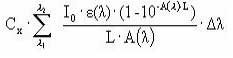
If A(λ )• L is below 0.02 then (1-10-A(λ )• L) » 2.3• A(λ)• L simplifying the above equation into:
Iabs (photons/L/s) = 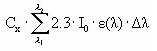
The quantum yield (Φ ), which is assumed to be independent of wave-length (which is an approximation) is then calculated from the measured photolytic half-life by:
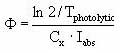
It should be ensured that the light intensity (I0) used in the above equations is the intensitity of the light actually reaching the solution, so the effects from the glass wall of the cuvette containing the test solution is excluded.
Metabolite data
This heading is only activated, if it is specified that metabolites are included in the simulation. Under this heading, all metabolite parameters are specified. These may be general physical or chemical properties of the metabolite, or related to processes in soil or in surface water. It is assumed that anaerobic conditions are present in the sediment of the phytoplankton dominated ponds and not in streams. Menues for specification of properties under anaerobic conditions are thus only present when ponds have been selected.
Basic chemical and physical properties
- Cas. No.
Chemical Abstracts Services registry number. The programme is reading the number as a text string.
- Mol weight (g/mol)
Specify the mol weight of the metabolite.
- Acid Properties
This refers to the pH dependent charge of metabolites showing basic or acid properties. Thus, for instance, metabolites containing the functional group of an amine might show basic or alkaline properties, whereas metabolites containing a functional carboxyl group show acid properties. Sometimes, it is difficult to evaluate, whether the substance has alkaline/neutral/acid properties. If the water solubility increases and/or the octanol-water partition coefficient decreases with pH, then the active substance has acid properties, if the water solubility decreases and/or the octanol-water partition coefficient increases with pH, then the substance has alkaline properties. Otherwise the substance is not expected to dissociate. An equilibrium between either a positive (alkaline) or a negative (acid) charged species and the neutral species will be present. Click off the right group.
- Henry's constant
If measured and if the substance is an acid or a base it should be ensured that the measured Henry's constant is for the neutral substance. The Henry's constant for a dissociating substance can be expressed by: H (neutral, dissociated) = α • H (neutral). If the Henry's constant is estimated, the field named "water solubility" has to be filled out. The field "vapor pressure" always has to be filled out, as this figure is used for the calculation of dry deposition. It should be noted that equation used for calculating the Henry's constant in general only holds for slightly water soluble substances.
- pKa
For acid and basic compounds, the pKa-value must be added to allow calculation of the amount of charged and neutral compound present for the pH-range of relevance for the soil.
- Log KOW:
The 10 logarithm to the distribution coefficient between octan-1-ol and water with the unit of KOW is (l/kg). If the substance is either acidic or alkaline, the log KOW of both the neutral and the charged part should be specified. In general, the log KOW of the neutral part is much higher than the log KOW of the dissociated part. At pH, where the degree of dissociation is low: KOW (neutral, dissociated) ~(1-α )·KOW (neutral). At pH, where the degree of dissociation is close to 1: KOW (neutral, dissociated) ~ a ·KOW (dissociated) + (1-α )· KOW (neutral).
If the dataset on corresponding values of log KOW and pH is not sufficient, the following empirical equation may be used:
log KOW (dissociated) » log KOW (neutral) - 3.5
- Water solubility (mg/l) at 20 degree Celcius.
The water solubility should only be provided for the neutral compound, since charged compound is considered as easily dissolved in water at the applied concentration of metabolite. The water solubility is pH-dependent for acidic and alkaline substances. At concentrations below concentrations, at which the dissociated part of the base or acid precipitate as salts, the measured solubility can be approximated by: SW = SWneutral/(1-α), where a is the dissociated fraction. The solubility of the neutral part (SWneutral) can be estimated from the above equation.
- Vapor pressure in the unit of Pa (Pascal).
The vapor pressure should only be provided for the neutral compound, since the evaporation of the charged compound is considered as negligible. The vapor pressure should be specified at 20°C. If the vapor pressure is specified at another temperature, then an appropriate way of extrapolating to 20°C is to assume that the temperature dependency of the vapor pressure can be expressed by the Antoine-like expression: Ln Psat = A - B/(t + 273), where A and B can be calculated from the measured vapor pressure and the boiling point (Psat = 101325 Pa at the boiling point).
Pesticide transformation to metabolite
- Transformation factor, P->M
The menu allows specification of how big a fraction of the degraded pesticide that is transformed to this metabolite for the different degradation process. If 80 out of 100 molecules are transformed to the metabolite in question, the fraction is 0.8.
- Relative molecular weight M/P
The relative molecular weight is calculated on the basis of the molecular weights specified for the pesticide and the metabolite.
- The conversion factor
The conversion factor is the product of the transformation factor and the relative molecular weight, and is used to calculate the mass of metabolite produced through degradation.
Metabolite in soil
The parameters to be specified under this heading relates to sorption and degradation of metabolites in a soil environment. To the largest extent possible, the formulation corresponds to what is used in the models recommended by the FOCUS-group on leaching to groundwater (FOCUS groundwater scenarios in the EU metabolite registration process), and the methods of parameter estimation given in their guidelines are recommended for use also for this model.
Sorption of metabolite in soil
- Choice of isotherm
The user must select whether to use a linear or a Freundlich sorption isotherm. It is recommended to use a linear isotherm - only if it is well documented that the Freundlich isotherm is well established for the lower concentration range of interest for leaching, should it be used. The default value for the exponent of a Freundlich isotherm is 0.9. The Freundlich isotherm is defined as x = Kfcref(c/cref)1/n, where x is the content of metabolite sorbed (mg/kg), and c is the concentration in the liquid phase (mg/l). cref is the reference concentration, which is usually 1 mg/l. K is usually given in dm3/kg (or l/kg).
- The sorption coefficient
The unit of the sorption coefficient must be dm3/kg (or l/kg). The sorption coefficient can be defined as a function of organic matter (KOM), as a function of organic carbon (KOC), as a function of clay (Kclay) or as a Kd-value of the soil. As % OC = % OM/1.724, KOC = KOM * 1.724. If KOC, KOM or Kclay is given, the sorption of each horizon in each soil profile is calculated as a function of the organic matter content or clay content of the respective horizon. The resulting values are shown in the spreadsheet of the menu. The equivalent Kd-value is the Kx * the fraction of the 'x' constitutent of the soil. If nothing else is known, sorption can be estimated from KOW in the following manner: log10(KOC) = 1.029*log10(KOW) – 0.18.
- Assistance to parameter choice
The following guidelines are specified in the report: FOCUS groundwater scenarios in the EU metabolite registration process:
"Soil sorption results (Kfoc, KOC or Kfom, KOM) are also required in four soils for parent compound and in three soils for relevant metabolites according to the environmental fate annexes to Directive 91/414/EEC (95/36/EC). Where these are all agricultural soils, the FOCUS group recommend that it is generally acceptable to use the mean value of the sorption constant normalised for organic carbon (Kfoc, KOC, KOM or Kfom) to derive the input to the model, unless the sorption is known to be pH-dependent. In situations where there are results from less than the recommended number of agricultural soils then it is generally appropriate to use the worst case result (lowest sorption). In cases where a large number of additional data points are available, a median value may be more appropriate. When characterising sorption behaviour of ionic compounds, the value will vary depending on the pH and a mean or median value is no longer appropriate. In this situation it is recommended that the choice of input parameter is made in relation to the pH of the soils in the scenario in the first instance.
In addition there will be certain compounds for which sorption and degradation are pH dependent and the values are linked (e.g. lower sorption at high pH but faster degradation). Under these conditions it is appropriate to use linked values of KOC and half life rather than average values of either. Inputs should be selected with the aim of obtaining a realistic rather than an extreme situation and the values used should be justified in the report.
For all model inputs derived from the regulatory data package, only studies of acceptable quality should be considered."
Degradation of metabolite in soil
- Half life
The degradation is specified as half life of the metabolite in days. The value has to be given according to a specific moisture content, which may be either pF 1 or 2, and with a reference temperature for the measurements. The default reference temperature is 20 oC, but the value can be changed by the user. Q10 is the relative increase in degradation rate with a 10 degree C increase in temperature. The default value is 2.2, equal to an exponent of 0.079, but other values of Q10 can be included.
In the model, the reference degradation rate is calculated as μ ref = ln2/(half life). The degradation rate is then modified according to temperature (Ft) and moisture content (Fw)according to the following formulas:
μ = μ ref* Fw*Ft, where
Ft = e α (T-Tref), α = ln(Q10)/10
Fw = (θ /θ b)0.7
- Distribution of degradation with depth
The degradation rates are modified with depth. The default values, according to the FOCUS report are 1 (0-30 cm depth), 0.5 (30-60 cm depth), 0.3 (60-100 cm depth) and 0 below 1 m's depth.
- Assistance to parameter choice
The environmental fate annexes to Directive 91/414/EEC (95/36/EC) recommend that degradation rate studies are undertaken in four soils for the parent compound and three soils for relevant metabolites (laboratory studies initially and then, if necessary, field studies). Therefore the FOCUS group recommend that where the parent compound has been studied in a minimum of four soils it is generally acceptable to use the mean degradation rate as input into the model. Similarly, the FOCUS group recommend that where the relevant metabolite has been studied in a minimum of three soils it is generally acceptable to use the mean degradation rate as input into the model.
In cases where a large number of additional data points are available, a median value may be more appropriate. In some cases the range of the results may be too large for this to be acceptable. This should be judged on a case by case basis and in this situation a value from a single study should be used, with appropriate justification of the study chosen.
In situations where less than the recommended number of soils have been studied it is generally appropriate to use the worst case result which is generated in a soil of agricultural use.
The FOCUS report recommends to calculate the degradation rate for each of the soils in the dossier at pF2, and to compare (and average) the values at this moisture content. The value found is then fed into the soils to be modelled, and modified according to moisture content and temperature within the model. This is the reason why degradation rates are not specified for each soil type in the catchments.
Metabolite in surface water
The parameters to be specified under this heading relates to sorption and degradation of metabolites in a lake or a stream environment.
Sorption of metabolite in surface water
Sorption relates to suspended material in the water or sediment at the bottom of the water body. The parameters to be specified for sorption can either be similar to what is given for the soil, or alternatively, KOC is calculated on the basis of KOW.
Degradation of metabolite in surface water
Degradation in surface water can be biological, or through hydrolysis or photolysis. For the phytoplankton dominated ponds it is necessary to specify both an anaerobic and an aerobic biological degradation rate since the sediment of the phytoplnakton dominated ponds is considered anarobic. The conditions in the stream are defined to be aerobic at all times. The reference temperature for the input has to be 20°C.
If only data on ready-biodegradability and/or inherently biodegradability data exist then it is suggested to used the recommended data from TGD (TGD: Technical Guidance Document. European Commission (1996): Technical guidance documents in support of the Commission Directive 93/67/EEC on risk assessment for new substances and the Commission Regulation EC 1488/94 on risk assessment for existing substances. Brussels, Belgium):
If the substance is ready biodegradable use a half-life of 15 days, if the substance i ready biodegradable, but failing 10-d window use a halflife of 50 days, if the substance is inherently biodegradable use a half-life of 150 days otherwise assume that the substance is persistent. The concentration of suspended matter should be set equal to 15 mg/L.
Aerobic metabolite degradation in surface water
Preferentially a total degradation rate for an experiment conducted as a shaking bottle experiment with suspended sediment (ISO 14952 Part 1) and the particle (suspended sediment) concentration at which the experiment was conducted should be entered. If the user prefer to use a degradation value obtained from a test without addition of suspended matter the particle concentration should be set to 0.
The reference temperature for the input has to be 20 oC.
Anaerobic metabolite degradation in surface water
These values are only relevant for phytoplankton dominated ponds. The values for anaerobic degradation are entered in the same way as the aerobic degradation.
Hydrolysis of metabolites in surface water
The model requires specification of acid, basic and neutral rates of hydrolysis at 20°C. The data request of the Danish EPA (Miljø- og Energiministeriet 1998) request that hydrolyis rates are determined in the interval of pH 4 to 9 and it should thus be possible to provide these rates through a solution of the above matrix system with repect to kacid, kbasic, kneutral. . Sometimes, it is not possible to use this strategy. For example, if it is specified that the no hydrolysis occurs at alkaline conditions, then kbasic should be set equal to zero, and if no hydrolysis occurs at acidic conditions, then kacid should be set equal to zero. If the rate of hydrolysis is almost independent of pH then kbasic and kacid should be set equal to zero, and the kneutral should be set equal to the measured rate of hydrolysis.
Photolysis of metabolites in surface water
Three types of parameters have to be specified:
- Quantum Yield
The quantum yield is the amount of compound degraded per quantum of light energy absorbed.
-Number of channels
Allows the user to specify the number of channels of the light absorption spectra.
- Standard Absorption Spectrum
The photolysis rate depends on the light absorption spectrum of the metabolite in the region of relevance to solar irridiation from 290 nm to 850 nm. It has been stated that the molar decadic absorption coefficient (L/mol/cm) has to above 10 at a wavelength above 295 nm if the direct photolysis is of relevance. The information on the standard absorption spectrum. This information is supposed to be part of the dossier for the pesticide. At each wavelength, the molar extinction coefficient has to be specified with the unit cm-1mol-1.
Very often quantum yield is not reported. Instead a measured photolytic half-life of a substance is obtained from experiments with a xenon lamp or other lamps with a specified light intensity (W/m2) (or outdoor experiments at a specified latitude and time of year). The characteristics of the lamp (energy distribution across the wavelength spectrum of the irradiation lamp) should be reported. If the experiments were carried out outdoors, the data on the energy distribution across the wavelength spectrum may be obtained from e.g. Zepp (Environ.Sci.Techn. 12, p. 327, 1978) and Frank (Chemosphere 10, p 985, 1988).
The amount of light intensity absorbed by the substance is calculated from (I0 is incident light intensity, L is the optical path length (cm), A is absorbance of the solution = ε • Cx, Cx is the concentration of the substance (mol/L), e is the molar decadic absorption coefficient (L/mol/cm), δ λ is appropriate wavelength intervals):
Iabs (photons/L/s) = 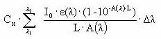
If A(λ )• L is below 0.02 then (1-10-A(λ )• L) » 2.3• A(λ )α L simplifying the above equation into:
Iabs (photons/L/s) = 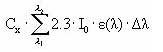
The quantum yield (Φ ), which is assumed to be independent of wave-length (which is an approximation) is then calculated from the measured photolytic half-life by:
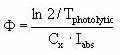
It should be ensured that the light intensity (I0) used in the above equations is the intensity of the light actually reaching the solution, so the effects from the glass wall of the cuvette containing the test solution is excluded.
Footnotes
[1] The first 2 hours after spraying, results are stored every 10 minutes. For the next 30 days, data are stored every hour. During the rest of the simulation, data are stored every 3rd day.
[2] Comment from reviewer: Given the event-driven nature of the pesticide exposure, the possibility to select different application dates will result in a wide range of calculated exposure concentrations for a specific crop. In my view it would be wise to limit the possibilities of selecting an application date or a very limited number of possible application dates.
[3] The programme presently uses the value given for Henry's constant and solubility for the pesticide also for the metabolite.
[4] The programme presently uses the value given for sorption for the pesticide also for the metabolite.
[5] The programme presently uses the value given for quantum yield and adsorption spectrum for the pesticide also for the metabolite.
Version 1.0 Maj 2004, © Danish Environmental Protection Agency