Pesticides Research no. 62, 2004
Calibration of Models Describing Pesticide Fate and Transport in Lillebæk and Odder Bæk Catchment
- 2.1 Deposition on Soil
- 2.2 Wind Drift
- 2.3 Dry Deposition
- 2.4 Soil Surface Processes
- 2.5 Processes in the Soil Matrix
- 2.6 Macropore- and colloid transport
- 2.7 Transport in drains and groundwater
- 2.8 Transport in the groundwater
- 2.9 Transport in streams
- 2.10 Sedimentation and re-suspension in ponds and streams
- 2.11 Diffusive exchange between the water column and the sediment
- 2.12 Sorption to sediment particles and suspended matter
- 2.13 Sorption to macrophytes
- 2.14 Biological degradation of pesticides
- 2.15 Photolytic degradation of pesticides
- 2.16 Evaporation of pesticides
- 2.17 Chemical or hydrolytic degradation of pesticides
- 3.1 Modelling water flow in the catchments
- 3.2 Modelling water flow in the stream models
- 3.3 Pesticide model for the catchment
- 3.4 Pesticide model for streams and ponds
- 3.4.1 Solar insolation
- 3.4.2 Dispersion
- 3.4.3 Suspended matter, temperature and pH
- 3.4.4 Biomass of macrophytes
- 3.4.5 Sediment bed
- 3.4.6 Sorption to sediment and suspended matter
- 3.4.7 Sorption to macrophytes
- 3.4.8 Biological degradation in pore water and water column
- 3.4.9 Biological degradation at macrophytes
4 Calibration and Validation of Water Flow
5 Calibration of Artificial Ponds
- 5.1 Calibration and validation
- 5.2 Process considered in the calibration
- 5.3 Calibration results
- 5.4 Verification of pesticide model for artificial ponds
- 5.5 Conclusion on the calibration and verification
6 Calibration and Validation of Pesticide Transport in the Catchment
- 6.1 Procedure
- 6.2 Simulation Results
- 6.3 Pesticide in drains
- 6.4 Uncertainty on the results caused by uncertainty on Koc and DT50
Appendix A - Water Balances and Issues related to Precipitation Data in the Odder Bæk-Catchment
Appendix B - Derivation of Parameters for the Unsaturated Zone
Appendix C - Pond Characteristics
Appendix D - Pesticide Characteristics used for the Pond and Stream Model
Preface
The project "Model Based Tool for Evaluation of Exposure and Effects of Pesticides in Surface Water", funded by the Danish Environmental Protection Agency (DEPA), was initiated in 1998. The aim of the project was:
To develop a model-based tool (PestSurf) for evaluation of risk related to pesticide exposure of surface water. The tool must be directly applicable by the Danish Environmental Protection Agency in their approval procedure. As part of this goal, the project had to:
- Develop guidelines for evaluation of mesocosm experiments based on a system-level perspective of the fresh water environment
- To develop models for deposition of pesticides on vegetation and soil.
- To estimate the deposition of pesticides from the air to the aquatic environment.
The project, called "Pesticides in Surface Water", consisted of seven subprojects with individual objectives. The sub-projects are listed in Table 1.
Table i Sub-projects of "Pesticides in Surface Water".
Tabel i Oversigt over delprojekter i "Pesticider i overfladevand".
| Title | Participating institutions | |
| A | Development and validation of a model for evaluation of pesticide exposure | DHI Water & Environment (DHI) |
| B | Investigation of the importance of plant cover for the deposition of pesticides on soil | Danish Institute of Agricultural Sciences (DIAS) |
| C | Estimation of the airborne transport of pesticides to surface water by dry deposition and spray drift | National Environmental Research Institute (NERI)
Danish Institute of Agricultural Sciences (DIAS) |
| D | Facilitated transport | DHI Water & Environment |
| E | Development of an operational and validated model for pesticide transport and fate in surface water | DHI Water & Environment National Environmental Research Institute |
| F | Mesocosm | DHI Water & Environment National Environmental Research Institute (NERI) |
| G | Importance of different transport routes in relation to occurrence and effects of pesticides in streams | National Environmental Research Institute (NERI) County of Funen County of Northern Jutland |
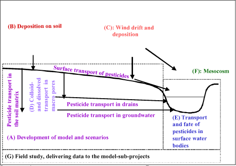
Figure i Links between the different sub-projects. The sub-projects are placed on a cross-section of the catchment to illustrate interactions.
Figur i Sammenhæng mellem delprojekterne. Delprojekterne er placeret på et tværsnit af en opland for at illustrere interaktionerne.
Figure 1 describes the relationship between the sub-projects. Sub-project 1 models the upland part of the catchment, while sub-project 5 models surface water bodies. Sub-project 8 delivers data to both modelling projects. Sub-project 2 and 3 develop process descriptions for spray drift, dry deposition and deposition on soils. Sub-project 4 builds and tests a module for calculation of colloid transport of pesticide in soil. The module is an integrated part of the upland model. Sub-project 6 has mainly concentrated on interpretation of mesocosm-studies. However, it contains elements of possible links between exposure and biological effects.
The reports produced by the project are:
- Styczen, M., Petersen, S., Christensen, M., Jessen, O.Z., Rasmussen, D., Andersen, M.B. and Sørensen, P.B. (2004): Calibration of models describing pesticide fate and transport in Lillebæk and Odder Bæk Catchment. - Ministry of Environment, Danish Environmental Protection Agency, Pesticides Research No. 62.
- Styczen, M., Petersen, S. Sørensen, P.B., Thomsen, M and Patrik, F. (2004): Scenarios and model describing fate and transport of pesticides in surface water for Danish conditions. - Ministry of Environment, Danish Environmental Protection Agency, Pesticides Research No. 63.
- Styczen, M., Petersen, S., Olsen, N.K. and Andersen, M.B. (2004): Technical documentation of PestSurf, a model describing fate and transport of pesticides in surface water for Danish Conditions. - Ministry of Environment, Danish Environmental Protection Agency, Pesticides Research No. 64.
- Jensen, P.K. and Spliid, N.H. (2003): Deposition of pesticides on the soil surface. - Ministry of Environment, Danish Environmental Protection Agency, Pesticides Research No. 65.
- Asman, W.A.H., Jørgensen, A. and Jensen, P.K. (2003): Dry deposition and spray drift of pesticides to nearby water bodies. - Ministry of Environment, Danish Environmental Protection Agency, Pesticides Research No. 66.
- Holm, J., Petersen, C., Koch, C. and Villholth, K.G. (2003): Facilitated transport of pesticides. - Ministry of Environment, Danish Environmental Protection Agency, Pesticides Research No. 67.
- Helweg, C., Mogensen, B.B., Sørensen, P.B., Madsen, T., Rasmussen, D. and Petersen, S. (2003): Fate of pesticides in surface waters, Laboratory and Field Experiments. Ministry of Environment, Danish Environmental Protection Agency, Pesticides Research No. 68.
- Møhlenberg, F., Petersen, S., Gustavson, K., Lauridsen, T. and Friberg, N. (2001): Guidelines for evaluating mesocosm experiments in connection with the approval procedure. - Ministry of Environment and Energy, Danish Environmental Protection Agency, Pesticides Research No. 56.
- Iversen, H.L., Kronvang, B., Vejrup, K., Mogensen, B.B., Hansen, A.M. and Hansen, L.B. (2003): Pesticides in streams and subsurface drainage water within two arable catchments in Denmark: Pesticide application, concentration, transport and fate. - Ministry of Environment, Danish Environmental Protection Agency, Pesticides Research No. 69.
The original thoughts behind the project are described in detail in the report "Model Based Tool for Evaluation of Exposure and Effects of Pesticides in Surface Water", Inception Report – J. nr. M 7041-0120, by DHI, VKI, NERI, DIAS and County of Funen, December, 1998.
The project was overseen by a steering committee. The members have made valuable contributions to the project. The committee consisted of:
- Inge Vibeke Hansen, Danish Environmental Protection Agency, chairman 1998-mid 2000.
- Jørn Kirkegaard, Danish Environmental Protection Agency (chairman mid-2000-2002).
- Christian Deibjerg Hansen, Danish Environmental Protection Agency.
- Heidi Christiansen Barlebo, The Geological Survey of Denmark and Greenland.
- Mogens Erlandsen, University of Aarhus.
- Karl Henrik Vestergaard, Syngenta Crop Protection A/S.
- Valery Forbes, Roskilde University.
- Lars Stenvang Hansen, Danish Agricultural Advisory Centre (1998-2001).
- Poul-Henning Petersen, Danish Agricultural Advisory Centre (2002).
- Bitten Bolet, County of Ringkøbing (1988-1999).
- Stig Eggert Pedersen, County of Funen (1999-2002).
- Hanne Bach, The National Environmental Research Institute (1999-2002).
October 2002
Merete Styczen, project co-ordinator
Sammenfatning og konklusioner
Pesticidtransport og nedbrydning er modelleret i to danske oplande. De to udvalgte oplande er repræsentanter for forskellige landskabstyper i Danmark, nemlig moræneler og sand. De er med i det nationale overvågningsprogram, og der eksisterer derfor et godt datagrundlag, der kunne udnyttes i arbejdet – dette var også en nødvendighed for udvælgelsen.
Formålet med modelleringen var altså at opstille og validere modeller for pesticidtransport og omsætning i de to oplande, for så senere at kunne modificere disse til scenarier i registrerings-sammenhæng.
Begge oplande er små, det lerede opland ca. 4.5 km2 og det sandede ca. 11 km2. For begge oplande er det betydende grundvandsopland anderledes end det topografiske opland. I det lerede opland er en stor del af randene åbne mod øst og vest, så vand løber ind upstrøms fra og ud via grundvandet i Storebælt. I det sandede opland er randene overvejende lukkede. Kun mod syd er der åbnet, hvor potentialekort og simuleringer tyder på, at vand dræner til vandløbet mod syd i stedet for at løbe til bækken.
Der er indsamlet data vedrørende klima, jordtyper, geologi, hydrogeologi, oppumpninger, arealanvendelse, pesticidanvendelse, pesticidegenskaber , vandløbsafstrømning, grundvandsniveauer og målte pesticidforekomster. Da de fleste målinger er punktmålinger, og modellen er tre-dimensional, er punktmålingerne tillægges en rumlig udbredelse. Modelsimuleringerne testes med hensyn til vand mod målte værdier for dræn- og vandløbsafstrømning samt grundvandsniveauer, og for pesticider mod pesticidmålinger i dræn og vandløb.
For at gennemføre undersøgelsen har det været nødvendigt at omfortolke nedbørsbeskrivelsen, jordtypernes fordeling og geologien i det sandede opland, mens der kun har været mindre justeringer af data i ler-oplandet.
I det lerede opland er overensstemmelsen mellem målt og simuleret afstrømning ved den nedre station meget god, og grundvandssvingningerne er rimeligt beskrevet, bortset fra i et område, hvor den geologiske fortolkning ikke stemmer overens med den observerede hydrologi. Den opstrøms station i det lerede opland er oversimuleret. Da den samlede mængde nedstrøms er korrekt, kan det skyldes at dræn er påhæftet lidt anderledes i forhold til målestationen end de er i virkeligheden, eller at vandet i den sydlige del løber sydpå i stedet for til den modellerede bæk, og at der så er overkompenseret for dette tab ved åbningen af randen mod Storebælt.
For det sandede oplands vedkommende, er alle stationerne oversimuleret lidt. Med de usikkerheder, der er med hensyn til nedbør, randenes faktiske placering samt afdræning sydpå, er det ikke muligt at komme meget tættere på de målte værdier. Der er et specielt problem med drænet i det sandede opland. Dels er drænets virkelige opland meget større end drænets geografiske placering, og dels må afstrømningen i sommerperioden skyldes indstrømning fra vandløbet (eller en anden ukendt kilde). Det synes ikke at være grundvand, da pejleboringerne viser at vandstanden falder under drændybde. Drænet er derfor uegnet til pesticid-valideringsformål.
Med hensyn til pesticid er simuleringer foretaget på to dræn samt opstrøms- og nedstrømsstationerne i det lerede opland, samt på hele det sandede opland.
Målingerne af pesticid på drænene er generelt meget lave, men for isoproturon er der en faktor 1000 forskel på målingerne fra begyndelsen af 1999 til slutningen af 2000. Disse variationer genfindes i simuleringerne.
For oplandene som helhed er resultaterne ikke helt så overbevisende. I det sandede opland er niveauet for de simulerede pesticidkoncentrationer nogenlunde korrekt, men de er langt mindre variable end de målte. Det skyldes primært to forhold. Det var ikke forventet at præferentielle strømninger spillede en stor rolle i det sandede opland, og dette var en forudsætning for valget af netop dette opland. De hurtige responser, der er observeret i oplandet tyder imidlertid på, at makroporer spiller en væsentlig rolle. Desuden synes fortyndingen i grundvandet at være for stor. Det giver sig udslag i at baggrundskoncentrationen stiger over simuleringsperioden og at koncentrationstoppene simuleret i vandløbet bliver for brede. Direkte dræning af lokalt mættede lag i den umættede zone forventes at ville forbedre beskrivelsen idet vand og stof ville forlade rodzonen "ufortyndet". Det ville føre til at toppene bliver smallere og den generelle baggrundskoncentration ville blive mindre.
For det lerede opland, hvor makroporer er inddraget i beskrivelsen, er simuleringen af pesticid-"toppene" i langt højere grad knyttet til nedbørstilfælde, som i observationerne. Men som i det sandede opland stiger baggrundskoncentrationen mere end i de observerede data. Desuden blev det klart at den valgte beskrivelse af kolloidtransport ikke er realistisk på oplandsskala. Beskrivelsen kræver, at makroporerne opfører sig som "nedløbsrør", for at kolloiderne kan nå ned til drænene. Sideeffekten af dette er, at for meget pesticid transporteres til grundvandet. Dette menes i høj grad at være medvirkende til de for høje baggrundskoncentrationer her.
Allerede tidligt i projektet blev det klart, at punktkilder kunne være en mulig fejlkilde i målingerne af pesticid i vandløbene, og at dette var en trussel mod valideringsøvelsen. Dette blev mere alvorligt end oprindeligt forventet. En analyse af de tre største fund i lerede oplands opstrøms station i 1999 viste høje fund af Terbutylazin, Diuron og Simazin. I det pågældende år er Terbutylazin kun anvendt på to, Diuron på en og Simazin på ingen marker opstrøms målestationen. Eftersom stofferne kun er brugt på små arealer (hvis overhovedet), og de samtidigt er fundet i høje koncentrationer (4.2 g/l i maj 1999), så viser en simpel tilbageregning, hvor der kun tages hensyn til fortynding, at koncentrationen under marken skulle have været i størrelsesordnen milligram/l, og ikke mikrogram/l, der ellers er det forventede niveau. Det tyder på at disse belastninger ikke skyldes markanvendelse, men punktkilder, der opstår i forbindelse med håndtering af pesticiderne. Over 50% af samtlige pesticidforekomster i det lerede opland er de tre stoffer, der er identificeret som punktkilder eller deres nedbrydningsprodukter. Også det største Diuron-fund nedstrøms i bækken i 1999 må udlægges som punktkilde, det samme gælder det absolut største fund i det sandede opland, nemlig 2.9 mikrogram/l Bentazon. Det faktum, at simuleringerne rammer det observerede niveau for disse stoffer kan derfor være misvisende.
For stoffer, hvor anvendelsen er udbredt, er det langt vanskeligere at skelne mellem punktkilder og belastning fra markerne. Alt andet lige, vil fortyndingen være mindre, og åkoncentrationerne derfor tættere på drænkoncentrationerne.
Summary and Conclusions
Pesticide transport and transformations are modelled in two Danish catchments. The two chosen catchments represent different landscape types in Denmark, that is moraine clay and sand. They are included in the national monitoring programme and a good database thus exists for each of them. The available data could be utilised for the work, and this was a necessary criterion for the selection.
The purpose of the modelling was thus to set up and validate models for pesticide transport and transformation in the two catchments, and later modify these to scenarios for use in registration.
Both catchments are small, the sandy loam catchment approximately 4.5 km2 and the sandy catchment approximately 11 km2. For both catchments, the groundwater catchment is different from the topographic catchment. In the sandy loam catchment model, the borders are open towards east and west, so water runs to the area from upstream and to the Great Belt via the groundwater. For the sandy catchment, the borders closed except towards the south where potential maps and simulations indicate that water drains to a stream to the south rather than towards the model stream.
Data are collected concerning climate, soil types, geology, hydrogeology, pumping, land use, pesticide use, pesticide properties, stream flow, groundwater levels and measured pesticide occurrences. Because most of the measurements are point measurements and the model is three-dimensional, the point measurements are given a spatial dimension. The model simulations are tested with respect to water and measured values for drain and streamflow and against groundwater levels, and for the pesticides against measurements in drains and streams.
To carry out the study it has been necessary to re-interpret the description of precipitation, the distribution of soil types and the geology in the Odder Bæk catchment, while less modifications of data were made for Lillebæk.
In the sandy loam catchment, the correspondence between measured and simulated values at the downstream station is very good and the groundwater fluctuations are reasonably well described, except in an area to the south where geological description is in disagreement with the observed hydrology.. The upstream station in sandy clay catchment is over simulated. As the total amount of flow downstream is correct this may be caused by the fact that the drains are connected to the river a slightly different in relation to the measurement station than it is in reality, or that water in the southern part runs south instead of towards Lillebæk, and that this loss is overcompensated through the open border towards the Great Belt.
With respect to the sandy catchment, all flow stations are somewhat oversimulated. With the uncertainties related to precipitation, the actual location of the borders and the drainage to the south, it is not possible to match the observations better. Special problems are found with respect to the drain in the sandy catchment. First, the actual catchment of the drain is much larger than it's geographical extent, and secondly the runoff during summer must be caused by inflow from the stream (or another unknown source). It does not appear to be groundwater, as the groundwater levels falls below drain depth. The drain is therefore not appropriate for pesticide validation.
With respect to pesticide, simulations are carried out on two drains, the up-and downstream stations in the sandy loam catchment and the downstream station in the sandy catchment.
The pesticide concentrations measured on the drains are generally very low, but for isoproturon, there is a factor 1000 difference between the measurements from the beginning of 1999 till the end of 2000. These variations are reproduced by the simulations.
For the catchments as a whole, the results are not quite as convincing. In the sandy catchment, the level of observed pesticide concentrations is simulated reasonably, but the simulated pesticide concentrations are much less variable than the measured. This is caused by two factors: It was not expected that preferential flow would play a large role in the sandy catchment – this was a pre-requisite for the selection of the catchment. The quick responses observed in the catchment imply that macropores play and important role. Furthermore the dilution in the groundwater appears to be too large. The result of this is that the background concentration increases over the simulation period and that the concentration peaks simulated in the stream become too wide. Direct drainage of the locally saturated layers in the unsaturated zone is expected to improve the description, because this would allow water and solute to leave the root zone without dilution. As a consequence, the peaks would be more condensed and the general background concentration would be less.
For the clayey catchment, where macropores are included in the description, the simulations of pesticide peaks are clearly linked to rainfall events, as in the observations. But as in the sandy catchment, the background concentration increases more than in the observed data. Furthermore, it became clear that the chosen description of colloid transport is not realistic at catchment scale. The description demands that macropores behaves as down pipes to ensure that the colloids reach the drains. The side effect of this is that too much pesticide is transported to groundwater. This is expected to be a major reason for the high background concentrations in the simulations.
Already early in the project is became clear that point sources could be a possible source of error in the measurement of pesticide in the streams and that this was a threat against the validation exercise. This became more serious than expected. An analysis of the three largest detections in the upstream station in 1999: Terbutylazin, Diuron and Simazin was carried out. In 1999, Terbutylazin was only used at two, Diuron at one and Simazin on no fields upstream of the measuring station. As the compounds are used on small areas only (if at all), and at the same time are found in high concentrations (for Terbutylazin, 4.2 microgram/l in May 1999), a simple calculation where only thinning is included, shows that the concentration under the root zone should have been in the order of milligram/l and not microgram/l which is the expected level. This indicates that these peaks are not due to field application but point sources created when pesticides are handled. More than 50% of the pesticide occurrences in the sandy loam catchment are the three mentioned compounds, identified as point sources, or their metabolites. Also the largest detection of Diuron downstream in the sandy loam catchment in 1999 must be classified as a point source, as there is no related use registered. The same suspicion exists for the largest detection in Odder Bæk, of 2.9 microgram/l of Bentazon. The fact that the simulations produce the levels of pesticide observed for e.g. Terbutylazin may therefore be misleading.
For compounds where the use is widespread, it is far more difficult to distinguish between point sources and field use. All else equal, the thinning will be less and the expected concentrations in the stream thus closer to the concentrations of the drains.
1 Introduction
The project "Pesticides in Surface water" concerns itself with formulation of a model for evaluation of transformations and transport of pesticides to surface water. The aim of the project is to produce a model to be used in the registration procedure.
Based on work carried out in the inception phase of the project (DHI et al., 1998, repeated in Styczen et al., 2004b), it was decided to base the model on existing representative 1. order catchments, in order to ensure that the parameterisation and weight given to the different processes would be realistic. This choice was based on
- an analysis of scale of different processes, and
- the need to be able to evaluate the effect of spraying of a field in combination with all the other activities taking place in the same catchment, influencing both the water flow in the stream and the background concentration of pesticide.
A model is therefore calibrated for each of the two selected catchments and the resulting setup is transformed to scenarios. The scenarios are packed with a special interface that only allows the user to change pesticide relevant parameters.
This report only concerns the calibration phase of the work.
1.1 Basic information on the selected catchments
The exact details of considerations leading to the choice of the catchments are described in the inception report (DHI et al, 1998). A key issue was that one of the catchments should represent moraine clay soil (soil type 5 and 6) and another sand soil (soil type 1 and 2)[1]. Together these soil types cover about 58% of the Danish arable area. According to the information available at the time, two catchments from the national monitoring programme (NOVA), with an adequate data availability could be selected to cover these conditions. No data set exists that represents soil type 3 and 4, making up 28% of the arable area.
The catchments Lillebæk on Funen (4.4 km2) and Odder Bæk in Northern Jutland (11.4 km2) were selected as study areas ( and ). Both catchments are included in the Nation-wide Monitoring Programme under the Action Plan on the aquatic Environment. The monitoring is presently carried out in both catchments under the programme "NOVA 1998-2003".
The soil types in the areas are shown in and the land use and distribution of crops in Table 1.2.
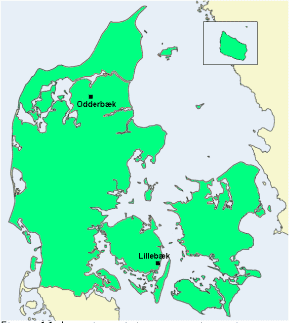
Figure 1.1 Location of the two study catchments.
Figur 1.1 De to modeloplandes geografiske placering.
Table 1.1 Distribution of soil types in Lillebæk and Odder Bæk catchments.
Tabel 1.1 Fordeling af jordtyper i Lillebæks og Odder Bæks oplande.
| jb.no FK |
1 1 |
2 2 |
3-4 3 |
5-6 4 |
7 5 |
8-10 6 |
11 7 |
Total | |
| Odder Bæk | in ha in % |
804 72 |
187 17 |
73 7 |
55 5 |
1119 101 |
|||
| Lillebæk | in ha in % |
17 4 |
404 96 |
421 100 |
Table 1.2 Existing Land Use in Odder Bæk and Lillebæk. The coverage of each land use type is given in %.
Tabel 1.2 Arealanvendelsen i Odder Bæks og Lillebæks oplande. Tallene er opgivet i %.
| Figures from 1997 | Odder Bæk | Lillebæk |
| Spring cereals | 25,1 | 21,2 |
| Winter cereals | 20,6 | 43,8 |
| Seeds | 1,2 | 21,0 |
| Pulses | 11,0 | 0,03 |
| Root crops | 4,5 | 2,10 |
| Grass and green fodder1 | 36,3 | 9,0 |
| Plantation and forest | 1,3 | 2,9 |
| Total | 100 | 100.03 |
| Continuous grass | 12,9 | 1,25 |
1 Please note that the permanent grassland is included in the statistics.
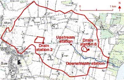
Figure 1.2 Lillebæk catchment, including 2 drain stations and 2 stream stations.
Figur 1.2 Lillebæk-oplandet, med angivelse af målestationer - to drænstationer og to afstrømningsstationer.
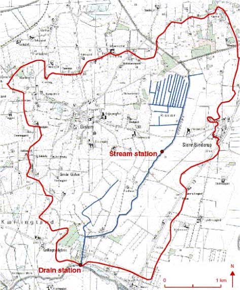
Figure 1.3 Map showing the Odder Bæk catchment with the stream and drain monitoring stations.
Figur 1.3 Kort over Odder Bæk-oplandet med å-og dræn-målestationer.
In the two catchments the following monitoring takes place every year
Lillebæk
- 6 soil moisture stations
- 6 double groundwater stations close to the soil moisture stations, with two bore holes in each of the depths 3 and 5 meters
- 9 separate groundwater stations were established. They were set with three filters on each station, but presently only 4 are in use. On three stations, one filter is in use and on the fourth station 2 filters are in use.
- 5 drain stations, of which 4 are connected with soil moisture stations
- 2 stream flow stations
- 1 weather station
Odder Bæk
- 6 soil moisture stations
- 12 groundwater stations close to the soil moisture stations, with two in each
- 12 separate groundwater stations
- 3 drain stations stream flow stations of which two were cancelled in 1993
- 2 weather stations. However, one is outside the map, approximately 2 km west of the catchment
In both catchments a questionnaire survey is conducted every year on farming practices at field level including information on spraying of pesticides (amount, time of year, etc.). The soil moisture station consists of ten Teflon suction cups. The cups are placed in a V-shaped pattern within an area of about 100 m2. The groundwater stations consist of three filters placed at approximately 1.5, 3 and 5 m below the surface. Furthermore, a monitoring well has been established near each groundwater station in the secondary groundwater occurrences, typically to a depth of 5-7 m, in Odder Bæk, however, to a depth of 20 m. Some deep wells may be present, with a filter depth down to 109 m.
In Lillebæk four pesticide monitoring stations are installed (). Two stream monitoring stations have been installed, one covering the water and pesticide loss from the entire catchment (436 ha) and one covering an upstream and culverted sub-catchment of approx. 230 ha. Moreover, two drain stations have been installed covering a field of 4.2 and 2.1 hectare, respectively.
In the Odder Bæk two pesticide monitoring stations are installed, consisting of one stream station covering the entire catchment (1143 ha) and one drain station covering a field of 32 ha ().
At all monitoring stations water stage is recorded continuously and stored on a data logger. Discharge is measured at regular intervals at every stream and drain station, which enables stage-discharge relationships to be established for the stream stations and V-notch weir-formulas in case of the drain stations. Thus, instantaneous discharge can be calculated for each station. Online access to the stage recorders is assured via connection to the telephone net, in case of the two drain stations in the Lillebæk via the mobile phone net.
The measurement programme was extended with a pesticide monitoring programme, which is described in Iversen et al. (2003).
1.2 Basic information on the two streams
Lillebæk is fairly steep and drops from approximately 50 m.a.s. (meter above sea level) to sea level over 3 kilometre. The upper half part of Lillebæk is submerged in pipelines, and the downstream part is open channel. The small tributaries are best described as ditches and the downstream part of Lillebæk as a small creek. Cross-sections have been measured in the downstream part – typically 1.5 meter wide and 0.5 meter deep.
In Odder Bæk the spring is found approximately 25 m.a.s. and drops over 4 kilometre to 10 m.a.s. Only one small tributary supplements Odder Bæk – the Gislum enge afløb, which is a pipeline. Cross-sections have been measured in Odder Bæk – typically showing 4-5 meter wide cross-sections of 1 meter depths.
Footnotes
[1] JB1: 0-5% clay, 0-20% silt, 0-50% fine sand, 75-100% sand in total, <10% humus
JB2: 0-5% clay, 0-20% silt, 50-100% fine sand, 75-100% sand in total, <10% humus
JB3: 5-10% clay, 0-25% silt, 0-40% fine sand, 65-95% sand in total, <10% humus
JB4: 5-10% clay, 0-25% silt, 40-95% fine sand, 65-95% sand in total, <10% humus
JB5: 10-15% clay, 0-30% silt, 0-40% fine sand, 55-90% sand in total, <10% humus
JB6: 10-15% clay, 0-30% silt, 40-90% fine sand, 55-90% sand in total, <10% humus
2 Model Descriptions Selected
- 2.1 Deposition on Soil
- 2.2 Wind Drift
- 2.3 Dry Deposition
- 2.4 Soil Surface Processes
- 2.5 Processes in the Soil Matrix
- 2.6 Macropore- and colloid transport
- 2.7 Transport in drains and groundwater
- 2.8 Transport in the groundwater
- 2.9 Transport in streams
- 2.10 Sedimentation and re-suspension in ponds and streams
- 2.11 Diffusive exchange between the water column and the sediment
- 2.12 Sorption to sediment particles and suspended matter
- 2.13 Sorption to macrophytes
- 2.14 Biological degradation of pesticides
- 2.15 Photolytic degradation of pesticides
- 2.16 Evaporation of pesticides
- 2.17 Chemical or hydrolytic degradation of pesticides
The modelling systems selected are MIKE SHE for the catchment and MIKE 11 for the streams. (DHI 2000a, 2000b, 2000c, 1997).
MIKE SHE is at present the only physically based, dynamic, fully distributed modelling tool for integrated simulation of all major hydrological processes occurring in the land phase of the hydrological cycle. The combination of a physically based and a distributed model enables a direct use of field data for model building and it enables linking to spatial data. The integrated approach makes MIKE SHE suitable for simulation of hydrologic systems where surface water and groundwater interactions are significant. An overview of MIKE SHE is shown in .
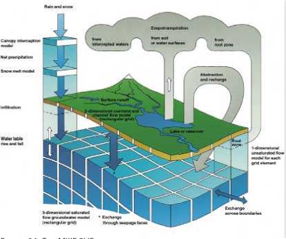
Figure 2.1 The MIKE SHE model, including a two-dimensional surface description, a one-dimensional unsaturated zone and a three-dimensional groundwater description.
Figur 2.1 MIKE SHE-modellen, indeholdende en todimensional overfladebeskrivelse, en en-dimensional umættet zone og en tredimensional grundvandsbeskrivelse.
The basic MIKE SHE module is the Water Movement module describing the hydrological processes. The hydrological components included are interception-evapotranspiration, infiltration, snow melt, 1-dimensional flow in the unsaturated zone, 3-dimensional ground water flow, overland flow in 2-dimensions and 1-dimensional stream flow, all of which are fully coupled.
The 1-dimensional stream flow is handled by the MIKE 11 model. MIKE SHE and MIKE 11 are dynamically linked. Exchange between the two models is described using 3 components – runoff, drainage and baseflow. The direct runoff is a result of water ponding on the terrain generating flow on the overland to the stream – the reverse process is also possible (stream flooding the terrain) – however, this is not applicable for these models. Drainage is generally used to describe the flow that takes place in drainpipes and small ditches to the stream. Finally the baseflow is the exchange between the stream and the groundwater. The water level and the groundwater level determine the direction of the flow – whether the stream is recharging or discharging the groundwater zone. Solutes are transported with the water and the basic transport is described with the MIKE 11 AD (advection-dispersion) module.
MIKE SHE can be extended with a module for solute transport by advection and dispersion (MIKE SHE AD), and different modules describing chemical reactions. For this particular work an extended version of the sorption/degradation module (MIKE SHE SD), including colloid transport, has been used.
With respect to the general description of the water flow, the models are unchanged. In order to model pesticide transport a number of process descriptions have been added. These are described in overall terms in the following. Details of specific process descriptions can be found in separate reports. The processes deposition on soil, wind drift, and dry deposition are not built into the version of the model used for calibration. However, results of the process descriptions are used either for estimation of input or evaluation of results. These processes are build into the final registration model, where conditions are more standardised than here.
The hydraulic transport processes considered, operating at catchment scale, are shown in . Transmission and transport processes operating at the level of ponds and streams appear from . These processes are implemented in a special MIKE 11 pesticide (PE) module developed through the project. The pesticide module is added on top of the AD and HD-module of MIKE 11 as illustrated on .
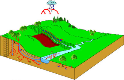
Figure 2.2 Schematic overview of pathways considered in the work. The compound may move as drift or dry deposition through the air. Along the surface, the compound may be transported with the water or on particles. In the soil, the compound may move through the matrix in soluble form or through the macropores as solutes or with colloids. The compound may move to groundwater and drains and from there to the stream. Plant uptake, degradation and sorption are possible processes. Sorption and degradation processes are also active in the stream.
Figur 2.2 Skematisk oversigt over de transportveje, der har indgået i arbejdet. Stoffet kan transporteres som drift eller tørdeposition gennem luften. Langs med overfladen kan pesticidet transporteres med vand eller på partikler. I jorden kan pesticidet bevæge sig gennem matricen i opløst form eller gennem makroporer som opløst stof eller med kolloider. Stoffet kan transporteres til grundvand og dræn og herfra til vandløbet. Planteoptagelse, nedbrydning og sorption er mulige processer. Sorption og nedbrydningsprocesser er også aktive i vandløbet.
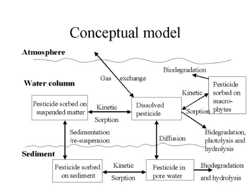
Figure 2.3 Conceptual drawing of transmission and transport processes for pesticides operating in streams and ponds.
Figur 2.3. Konceptuel oversigt over udvekslinger og transportprocesser for pesticider i vandløb og vandhuller.
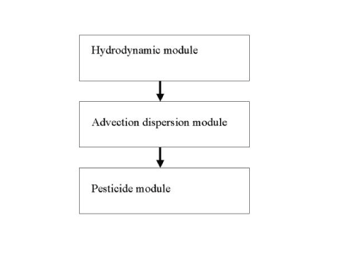
Figure 2.4 The connections between the modules of the MIKE 11 model.
Figur 2.4 Sammenhængen i MIKE 11's moduler.
2.1 Deposition on Soil
The amount of pesticide reaching the soil is, in these simulations, a function of the plant cover. The values used to estimate the actual deposition on soil for a given pesticide are "handpicked" from experiments carried out as part of the project (Jensen and Spliid, 2003), for winter wheat, barley, potatoes and sugar beet). For other crops, the data stem from the FOCUS groundwater report (FOCUS 2000).
2.2 Wind Drift
Wind drift is estimated according to Ganzelmeier. Based on an evaluation of wind speeds in Denmark compared to the conditions, under which the Ganzelmeier figures were derived, it is assumed that the 95% percentile of Ganzelmeier equals the average Danish conditions (Asman et al., 2003). The wind drift module developed for the scenario-runs has not been used in the model calibration phase, but wind drift has been taken into account when comparing results to observations.
2.3 Dry Deposition
Dry deposition is estimated according to the procedure described in Asman et al. (2003). Dry deposition is the result of the emission of pesticide from the soil or crop surface. The emission is an input in the dry deposition, also calculated by the procedure. The estimated deposition in the stream takes place over seven days of 21 days, depending on whether the deposition takes place from a plant cover or a bare soil. The calculation is carried out for average climatic conditions. The dry deposition module developed for the scenario-runs has not been used in the model calibration phase. It has, however, been considered when comparing results to observations.
2.4 Soil Surface Processes
Water that does not infiltrate may flow on the soil surface to a surface water body or infiltrate along the way if conditions allow. Initially, it was the intention that soil erosion would be included in the model as a mean of transport for pesticide. However, during the two observation years, erosion was not observed in the catchments, and simulations produced hardly any surface flow. It was therefore decided not to include the description in the final model.
2.5 Processes in the Soil Matrix
Water infiltrates from the surface to the saturated zone through the soil matrix or through macropores. Water movement in the matrix is described with Richards' equation. The physically based description of macropore flow assumes a secondary pore domain through which water is routed separately, but allowing exchange with the surrounding bulk porosity (or matrix porosity). Evaporation takes place by uptake through plants (transpiration) and through the soil surface. In the matrix, pesticide can be adsorbed according to a linear or a Freundlich isotherm, and both the adsorbed and the soluble form of the pesticide can degrade (1. order). Plant uptake of pesticide is defined as a fraction of the transpiration stream (DHI 2000).
The transport of solutes in the saturated zone is governed by the advection-dispersion equation, which for a porous medium with uniform porosity distribution is formulated as follows:
where c is the concentration of the solute, Rc is sources or sinks, Dij is the dispersion coefficient tensor and vi is the velocity tensor.
The advective transport is determined by the water fluxes calculated during a MIKE SHE WM simula.tion. In order to determine the groundwater velocity the Darcy velocity is divided by the effective porosity:
![]()
where qi is the Darcian velocity vector and θ is the effective porosity of the medium.
Volatilisation is not described explicitly in the model. However, the emission from leaves and the soil surface used in the description of dry deposition is likely to take into account part of this effect.
2.6 Macropore- and colloid transport
Water may move from the soil surface or the soil matrix to the macropore domain, if it is present as free water on the soil surface, or if a pressure builds up in a particular layer in the soil. Water re-infiltrates from the macropore to the matrix as a function of pressure differences between the two domains. Pesticides move with the water from the surface or the matrix to the macropore and back, and thereby bypass the soil matrix. In addition, colloid transport has been added to the description (Holm et al., 2003). Soil particles can be loosened by rain and follow the water into the macropores or soil matrix. The particles will be filtered from the flow in the matrix but only to a limited degree in the macropores. The study on colloid transport (Holm et al., 2003) recommended that the transport out of macropores was set to 0. As these particles can interact with pesticides (mainly with a high Kd-value), they may act as a transporting agent for pesticides.
2.7 Transport in drains and groundwater
The model description includes drains, which are activated when the groundwater level raises above the level of the drains. Drainage cannot be generated from layers above the groundwater. In reality, however, drainage can be generated from perched water tables, but this is not included in the model. The concentration of the water moving in the drain is equal to the concentration in the uppermost calculation layer of the saturated zone in the model. Water is routed from the saturated zone to the drain with a drainage constant (linear reservoir description).
2.8 Transport in the groundwater
Transport in the groundwater is described in a three-dimensional network. Flow of water is described by the 3-D Boussinesq Equation for saturated flow. Water and solute enters the groundwater from above as recharge from the unsaturated zone, and may leave the zone either through the drain (from the uppermost layer of the groundwater) or by flowing to the stream. In principle, both degradation and sorption of pesticide may take place in the groundwater zone. However, through the parameterisation degradation is set to zero in the groundwater zone. This is the recommendation given by FOCUS for pesticide registration purposes (FOCUS, 2000).
2.9 Transport in streams
The HD (hydrodynamic) module of MIKE 11 contains an implicit, finite difference computation of unsteady flows in rivers and estuaries. The formulations can be applied to branched and looped networks. The computational scheme is applicable to vertically homogeneous flow conditions ranging from steep river flows to tidally influenced estuaries. Both sub-critical and supercritical flow can be described by means of a numerical scheme, which adapts according to the local flow conditions. The complete non-linear equations of open channel flow (Saint-Venant) can be solved numerically between all grid points at specified time intervals for given boundary conditions.
2.10 Sedimentation and re-suspension in ponds and streams
Pesticides adsorbed to suspended particles in the water column might be transported to the sediment when suspended particles settle. Similarly, pesticides adsorbed to particles in the sediment might be transported to the water column when re-suspension of sediment occurs. Hence the net result of theses process is a function of the concentrations of pesticides sorbed to particles in sediment and water column and the re-suspension and sedimentation rates. These processes are implemented in the MIKE 11 model, but data for the dynamics of the sediment is generally not available for the two catchments. It was therefore decided to set the exchange of sorbed pesticides between the water column and the sediment to 0. For ponds this decision is supported by experiments with artificial ponds, which showed that transport of pesticides by sedimentation was insignificant compared to the transport by diffusion (Mogensen et al., 2004).
2.11 Diffusive exchange between the water column and the sediment
According to (DHI et al., 1998) the sediment in the streams is assumed to be well mixed and of a thickness of about 2 cm (Styczen et al., 2000b) and the sediment should therefore be described by a single box. The assumptions for this was that the sediment is supposed to undergo frequent minor re-suspensions even through calm summer conditions and that water entering the stream from the catchment is supposed to penetrate the sediment. As a consequence the sediment is supposed to be well mixed with regard to the concentrations of pesticides and a one-layer model of the sediment is therefore considered as appropriate.
The sediment of the ponds was assumed (DHI 1998 and Styczen et al., 2000b) not to undergo re-suspension as frequent as in the streams and the sediment might be stratified with regards to the concentrations of pesticides due to diffusion. To describe this diffusion numerically the sediment layer has to be divided in to multiple layers to allow a description in accordance with Ficks second law (Styczen et al., 2004c).
2.12 Sorption to sediment particles and suspended matter
The pesticide in the water column and in the sediment bed might either be sorbed to particles or dissolved. In the water column this sorption is assumed to be kinetic and the kinetics was described by a (pseudo) first order sorption rate and a first order desorption rate. This description implies that the sorption is considered as reversible, which was verified by the sorption experiments of (Helweg et al., 2003).
To implement this description of diffusion relying on Ficks second law (see section ) it was for logistic reasons necessary to describe the sorption in the sediment of the ponds by an equilibrium approach. However, diffusive processes occurring at a length scale of less than 1 mm might resemble the process of kinetic sorption. Hence it can be argued that the kinetic of sorption in the sediment is lumped in to the effective diffusion coefficient derived through the calibration exercise (section 5).
2.13 Sorption to macrophytes
The pesticide in the water column might also sorb to macrophytes. As for the sorption to sediment particles and suspended matter the sorption to macrophytes was described by a first order sorption and a first order desorption rate.
2.14 Biological degradation of pesticides
Pesticides in the porewater of the sediment and dissolved in the water column are assumed to undergo biological degradation. In every case the biodegradation are formulated as a first order degradation. The temperature influence on biodegradation was described by an Arrhenius equation.
2.15 Photolytic degradation of pesticides
The dissolved pesticide in the water column might undergo photolytic decay, which in theory might be either direct or indirect. Direct photolysis takes place if the chemical absorbs light, and as a consequence, undergoes transformation. Indirect photolysis takes place if the chemical receives energy from another excited species (sensitised photolysis) or very reactive, short-lived species (e.g. peroxy-radicals, singlet oxygen), which are formed due to absorption of light by dissolved organic materials (Schwarzenbach et al 1993). All though descriptions of the formulation of indirect photolysis are available from the literature (Schwarzenbach et al 1993) implementation of indirect photolysis in the stream model was considered as irrelevant. Thus the parameterisation of the process of indirect photolysis requires a detailed knowledge about the chemical composition of the organic mater of the stream water which not is readily available. As a consequence the total photolytic degradation might be underestimated. The photolytic degradation was described as a first order decay.
The first order photolytic decay rate was calculated as a function of the intensity and the spectral composition of the light and the light attenuation in the water column, which depends on the concentration of suspended matter and on the light absorption spectra of the pesticide. The light attenuation in the water column was estimated as a part of the calibration exercise.
2.16 Evaporation of pesticides
Evaporation of pesticides from the water column to the atmosphere is described by the same equations as used for description of the dry deposition of pesticides from the atmosphere to the water column (section ).
2.17 Chemical or hydrolytic degradation of pesticides
Hydrolysis of the dissolved pesticide in the water column and the pore water were described as a first-order reaction given by (Schwarzenbach et al., 1993). The hydrolysis rate constant may include contributions from acid- and base-catalysed hydrolysis as well as nucleophilic attack by water.
3 Model Setup
- 3.1 Modelling water flow in the catchments
- 3.2 Modelling water flow in the stream models
- 3.3 Pesticide model for the catchment
- 3.4 Pesticide model for streams and ponds
- 3.4.1 Solar insolation
- 3.4.2 Dispersion
- 3.4.3 Suspended matter, temperature and pH
- 3.4.4 Biomass of macrophytes
- 3.4.5 Sediment bed
- 3.4.6 Sorption to sediment and suspended matter
- 3.4.7 Sorption to macrophytes
- 3.4.8 Biological degradation in pore water and water column
- 3.4.9 Biological degradation at macrophytes
In the following, a description is given of the specific data included in the Lillebæk and Odder Bæk models. As the final data choice in some cases builds on considerable analysis, the main issues are summarised in the following sections and the details are given in appendices.
3.1 Modelling water flow in the catchments
3.1.1 Discretisation
Both models are established in a 50-meter grid – i.e. each calculation cell measures 50x50 meter. Given the catchment areas to which the model areas where adopted the number of boundary cells and internal calculations cells equal (178/1849) and (243/3929) per layer for Lillebæk and Odder Bæk respectively. The vertical discretization is set to reflect the geological model – i.e. the calculation layers are set equal to the geological layers. For the unsaturated zone, the discretisation is fine near the surface and coarser towards the groundwater table. In Lillebæk the cell height is between 2.5 and 5 cm in the A and B horizon, and between 5 and 50 cm in the C horizon. In Odder Bæk the discretisation has not been strictly linked to the horizon but more controlled by the depth resulting in 2.5 to 10 cm cell height in the A horizon, 5 to 10 cm in the B horizon, and 20 to 50 cm in the C horizon.
3.1.2 Boundary conditions
In the upstream end of the Lillebæk catchment, water flows into the area since a groundwater divide can be identified outside the model area – found using a map of groundwater potentials provided by the county of Funen. In the downstream end outflow through a white sand layer is expected to take place towards the sea (Dansk Geofysik, 2000; DGU, 1989a). Where the groundwater flow is expected to take place across the boundary, boundary conditions are described using the option constant hydraulic pressure where. Furthermore, modifications had to be made for the sand lens (see the chapter on geological description, 3.1.6). Evaluating the extent of the lens, the surface topography and the topology of the Hammersbro Bæk just south of the Lillebæk model it is found that flow is likely to take place in the lens towards Hammersbro Bæk. For a proper boundary description knowledge of the potentials in the lens would be of most importance. No direct information is available and it was chosen to fixate the potential head in the lens east of Oure town – over 750 meters going from 34 m.a.s in west to 24 m.a.s. in east.
The boundary of the Odder Bæk model is slightly modified compared to the surface catchment area. To the north the boundary is adjusted to match the groundwater divide. From the two hydro-geological reports (DGU, 1989b, Nordjyllands amt, 1998), the following assumptions with regard to groundwater were adopted:
- Groundwater flow in the upper aquifer is most likely routed towards the stream
- The lower aquifer has a larger extent than the small Odder Bæk stream catchment and groundwater flow is assumed flow from north to south.
- There may be contact between the two aquifers in parts of the catchment
- Based on head observations in the upper aquifer, it is likely that an east-west groundwater divide is located north of Gislum.
By running the model with different boundary conditions the most probable direction of groundwater flow in the upper aquifer was estimated. In this way, the model itself was used to establish the most probable groundwater catchment for the upper aquifer, and a new catchment was established which are smaller than the topographical catchment and more smooth around the corners (Figure 3.7).
Finally, the southern border was opened to allow water to move towards the stream to the south. This last change is in correspondence with a map of hydraulic potential made available by the county of Northern Jutland and improved the simulations of groundwater variations in the southern part of the Odder Bæk catchment.
3.1.3 Climatic variables
The choice of climatic parameters is not entirely consistent. This is mainly caused by several changes in recommendations from the concerned institutions over the time of the project, and differences in data availability in the two catchments.
For Lillebæk, precipitation is measured in the catchment during the whole period of the project (station: Bolsmose). In addition, rainfall intensity (per 15 minutes) is measured at a special station in the catchment from mid 1999 till the present. The measurements of precipitation are corrected, using the (new) standard correction factors (Allerup et al., 1998). Climatic parameters for calculation of evaporation are measured at a nearby research station (Aarslev). Evaporation is calculated according to Makkink (Aslyng and Hansen, 1982).
It should be noted that the Lillebæk catchment and the drain stations have been the object of other model studies. An analysis of earlier simulations for the catchment showed considerable differences between climatic datasets chosen, partly due to selection of different data sources and partly due to errors in the data sets. The results presented here are therefore not necessarily similar to what has been presented earlier from NOVA (the National Monitoring Programme).
For Odder Bæk, the choice of climatic data went through several iterations, see Appendix A. The precipitation record finally selected is grid precipitation from DMI for grid no. 10215, modified with the correlation (P = 0.926 * Pgrid, R2 = 0.96). This generated series is then corrected, using the dynamic correction factors from Vejen et al. (2000) and (2001). Evaporation is calculated according to Makkink, for the same grid.
Due to the fact that macropores are included in the description in Lillebæk, data from the rainfall intensity station 28184 on Funen was analysed. It is the intensity station that resembles the Bolsmose station the most. Data was summarised for every 6 minutes, and the record corrected so that the monthly rainfall is identical to the rainfall at the Bolsmose station. This is not entirely correct, because one of the differences between the station types is that very small events are not measured by the intensity stations. With this correction method, the lacking rainfall is added to the measured events through scaling of the measured events. It was, however, the only possible way to create a record with realistic intensities for the whole of the measurement period. This high intensity rainfall was only used in the scenarios, while the calibration of the water flow was done on daily values. For the calibration of pesticide transport, however, the model was run with the intensity record in order to generate macropore flow and colloids.
3.1.4 Vegetation parameters
Within the two catchment areas of forest, wetlands, urban/fallow and arable lands were mapped. In the arable lands different crop are represented – winter cereal, spring cereal, pea, beet, potato, and grass – and randomly distribution of the crops was performed.
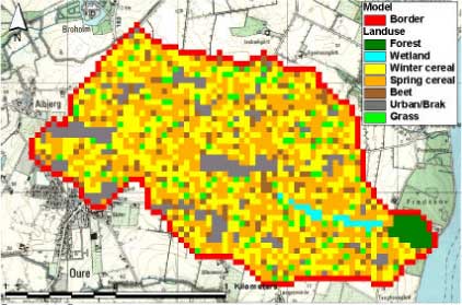
Figure 3.1 Distribution of vegetation in the Lillebæk model.
Figure 3.1 Arealanvendelsen i Lillebæk-modellen.
Figure 3.2 Distribution of vegetation in the Odder Bæk model.
Figur 3.2 Arealanvendelsen i Odder Bæk-modellen.
The MIKE SHE water model requires data about the development of leaf area index and root depth for each crop or vegetation. These are derived from (Plauborg, F. Olesen, 1991) for the agricultural crops.
Inception and transpiration is described as a function of root depth, root distribution and leaf area index in the model. However, experience has shown that transpiration exceeds potential evaporation under certain conditions. To account for that, the potential evaporation is multiplied with 1.25 for permanent grass along the stream (wetland), and with 1.1 for crops during the period of maximum vegetative growth. This is in line with the general recommendations of FAO for calculation of evapotranspiration for crops, and it is believed to be in line with the new recommendations for calculation of evapotranspiration under Danish conditions (Plauborg et al., 2002).
3.1.5 Soil parameters
The sources of soil information for the two catchments are: Soil profile descriptions carried out for six profiles in each catchment (Nielsen, 1998, Nielsen, 1999, Jensen and Madsen, 1990), soil maps from Foulum ("Jordklassificering, Danmark, Basisdatakort, 1:50.000-JB 1312 11 NØ (Lillebæk) and similar maps made available by the County of Northern Jutland), soil type maps from GEUS describing the soil material in 1 m's depth, and to some extent information from geological boreholes and geophysical measurements of the two catchments.
For Lillebæk, the soil map of the plough layer is almost uniform for the whole catchment. The map of 1 m's depth shows sandy underground in the eastern end of the catchment. This corresponds well with the geological interpretation of the catchment in general and with the soil profiles described. The easternmost profile shows sand at depth. However, in spite of the fact that the catchment appears uniform on the maps, the hydraulic parameters measured differ from profile to profile. To catch the variation in the model, parameters from the 5 profiles analysed are distributed randomly in the uniform area, while parameters from the 6th profile are used for the area with sand at depth. Macropores are included in the description. They make up 1% of the volume of the soil. Key parameters for each soil are shown in Appendix B.
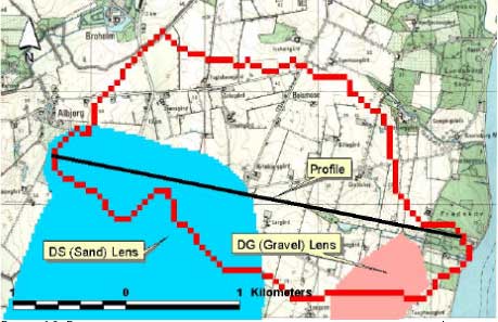
Figure 3.3 Map showing the distribution of the soil types used in Lillebæk and the locations of the measured soil profiles (St. 1-6). Profile 1-5 are distributed randomly, while profile 6 is used in areas where the geology indicates sand at 1 m's depth.
Figur 3.3 Kort over fordelingen af jordtyperne i Lillebæk og placeringen af de målte profiler (St 1-6). Profilerne 1-5 er tilfældigt fordelt mens profil 6 anvendes i den del af arealet hvor geologien indikerer sand i 1 m's dybde.
The interpretation of soil types in Odder Bæk was less straightforward. Topsoil parameters in terms of soil texture, retention curves and saturated hydraulic conductivity have been measured at 6 locations within the catchment (black dots on Figure 3.4 with measured top- and subsoil texture class (JB)). Comparing the measured data with the available map of topsoil classes shows that only 3 of the 6 measured data sets match the map classification. Some of the profiles show rather heavy textures at depth. To improve the understanding, an effort was made to interpret the geological borehole data of the area. A clay layer was identified which varies from 0.5 metre to 42 metre below the soil surface with a thickness varying between 1 and 26 metre. In addition, a local appearance of clay deposits close to the soil surface, oriented east-west, has been identified in the middle of the catchment. The thickness of this deposit varies between 0 and 15 m. The soil map finally generated is thus somewhat different from the original.
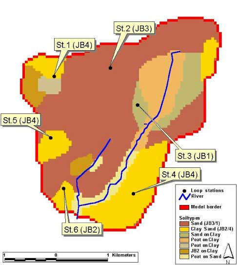
Figure 3.4 Map showing the distribution of the soil types used in Odder Bæk and the locations of the measured soil profiles (St. 1-6).
Figur 3.4 Kort over den anvendte jordtypefordeling i Odder Bæk og placeringen af de beskrevne profiler.
The hydraulic parameters used for the different zones were initially based on measured values, but some values were changed during calibration. Initially, the measured values from station 2 represented the soil type "Sand" but it was not possible to reproduce the measured variations in groundwater levels corresponding to the measured values with this rather extreme retention curve. The values finally selected are described in Annex B. No measurements were available to represent the organic soils present in the catchment. General parameters from literature were therefore used (Annex B).
3.1.6 Geological description and hydraulic parameters
For Lillebæk, the geology is described on the basis of geological borehole data from the ZEUS geological database. Secondly, during the spring 2000, the county of Funen mapped the area by means of geophysical measurements (Dansk Geofysik, 2000) providing an excellent extension of data available for geological interpretation. Thirdly, the utilisation of the geological interpretation tool, GeoEditor (DHI, Water & Environment, 2000), has made a simultaneous interpretation possible from both geological borehole information and geophysical data.
The interpretation has been conducted at DHI, but the County of Funen has played an important role in the verification of the model by providing geological experience along with previously interpreted profiles.
The adopted interpretation procedure was to import the borehole database in the GIS-based GeoEditor, and construct geological profiles. Three of the profiles match interpreted profiles by the County of Funen, another 15 of the profiles match geophysically interpreted (TEM) profiles by Dansk Geofysik (2000), and seven of the profiles were oriented west east to cover the overall area mainly with respect to the boreholes. The geological layers were afterwards interpolated on the basis of the digitised profiles.
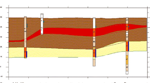
A three-layered geological model was established – with a sequence from surface of moraine, white sand and tertiary clay. Two major lenses of sand and gravel are encapsulated in the moraine clay. The extents of the lenses are shown in , and a west-east cross section of the geological model is shown in . The upper sandy lens (a secondary aquifer) consists of diluvial sand, whereas the lower sandy (primary aquifer) consists of interglacial sand. The main orientation of the sandy deposits is horizontal. In most of the area the lower sandy aquifer is underlain by tertiary clay (Kerteminde mergel) forming an aquitard of very low permeability. The approximate location of the bottom of the lower sandy aquifer is 0-10 m below sea level. The thickness of the primary aquifer typically varies between 8 and 16 m, but increases to 20-30 m to the very west and decreases to 0 m to the very east of the area.
The hydraulic conductivities applied in the model are listed in .
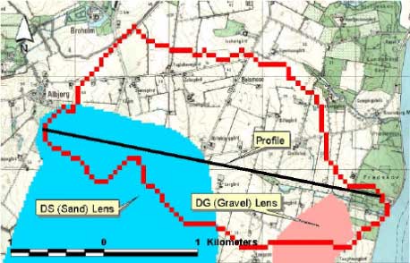
Figure 3.5 Extent of gravel and sand lenses in the moraine clay layer in Lillebæk.
Figur 3.5 Udbredelsen af grus- og sandlinser i morænelers-området i Lillebæk.

Figure 3.6 West-East geological profile in Lillebæk along the line indicated in Figure 3.5.
Figur 3.6 Geologisk profil i Lillebæk gennem linien vest-øst indikeret i figur 3.5
Table 3.1 Parameters applied for the geological formations in Lillebæk. For the top calculation layer the storage capacity values are automatically adjusted by values specified in the unsaturated zone.
Tabel 3.1 Parametre anvendt til beskrivelse af de geologiske formationer i Lillebæk. For det øverste beregningslag er porevoluminet automatisk justeret med værdierne specificeret for den umættede zone.
| Formation | Conductivity | Storage Capacity (-) |
Specific Yield (-) |
|
| Horizontal (m/s) | Vertical (m/s) | |||
| Moraine | 4.37e-6 | 4.37e-7 | 0.2 | 0.001 |
| White Sand | 1.36e-5 | 1.36e-6 | 0.3 | 0.002 |
| Tertiary Clay | 3.74e-6 | 7.48e-8 | 0.2 | 0.001 |
| Sand Lens | 8e-5 | 4e-5 | 0.3 | 0.002 |
| Gravel Lens | 8e-5 | 4e-5 | 0.3 | 0.002 |
With respect to Odder Bæk, the area is not well enough covered by deep boreholes to create a reliable geological model only from boreholes. Thus, geophysical data have been employed in the interpretation.
The geological model has been established on the basis of two reports on hydro-geological mapping (DGU, 1989b; Nordjyllands Amt, 1998), together with borehole data extracted from the geological database (ZEUS) at GEUS. The adopted interpretation procedure was to import the borehole database in a GIS-based GeoEditor, and construct geological profiles which as close as possible match 7 interpreted profiles, which are presented in the latter of the mentioned reports. The geological layers were afterwards interpolated on the basis of the digitised profiles.
The outcome of the process is a geological model with 2 sandy aquifers divided by a clay layer. The bottom of the model is the top of a thick clay layer located underneath the two sandy aquifers, approx. 20 m below sea level. In the geological reports a third deep aquifer has been identified (approx. 70 m below sea level), but as this will not be in contact with the stream, Odder Bæk, it has been excluded from the model setup. The position of the clay layer varies from 0.5 m to 42 m below surface with a thickness varying between 1- 26 metre. In addition, a local appearance of clay deposits close to the soil surface has been identified in the western part of the catchment – beneath a small lake. This deposit has been included in the model as a lens with specified extent – shown in and in cross section in Figure 3.8.
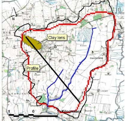
Figure 3.7 Extent of clay lens in the top sand layer in Odder Bæk. The black curved line shows the topographical catchment, while the red "box"-line shows the actual model area.
Figur 3.7 Udbredelse af lerlinse i det øverste sandlag i Odder Bæk. Den sorte kurvelinie viser det topografiske opland mens den røde "kvadrat-linie" viser det faktiske modelområde.
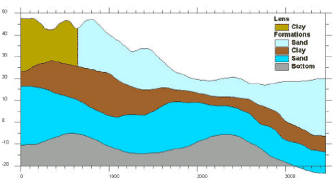
Figure 3.8 NWest-SEast geological profile in Odder Bæk along the line indicated in Figure 3.7.
Figur 3.8 Geologisk profil i Odder Bæk gennem linien nordvest-sydøst indikeret i Figur 3.7.
Table 3.2 Parameters applied for the geological formations in Odder Bæk. For the top calculation layer the storage capacity values are automatically adjusted by values specified in the unsaturated zone.
Tabel 3.2 Parametre anvendt til beskrivelse af de geologiske formationer i Odder Bæk. For det øverste beregningslag bliver porevoluminet automatisk justeret med værdier specificeret for den umættede zone.
| Formation | Conductivity | Storage Capacity (-) |
Specific Yield (-) |
|
| Horizontal (m/s) | Vertical (m/s) | |||
| Top Sand | 1.03e-5 – 1.25e-4 | 12/100*Kh | 0.3 | 0.0004 |
| Clay | 4.00e-7 | 8.00e-8 | 0.35 | 0.0005 |
| Bottom Sand | 2.00e-5 | 1.00e-5 | 0.3 | 0.0004 |
| Clay Lens | 1.4e-7 | 1.60e-7 | 0.35 | 0.0005 |
The overall impression of the geological interpretation is that the area is rather complex with respect to groundwater flow with clay deposits located near the soil surface in 15-25% of the area. The hydraulic conductivities have for the top sand been specified as distributed values, with a ratio between horizontal and vertical values of 100/12. The distribution is shown in Figure 3.9
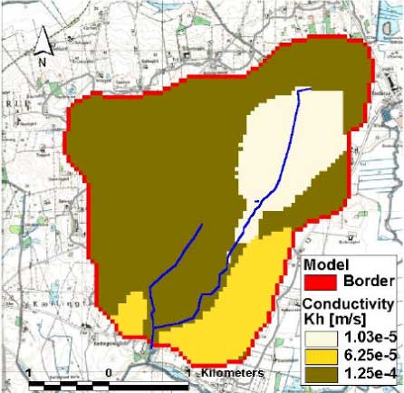
Figure 3.9 Horizontal conductivity in top geological layer in Odder Bæk. The vertical conductivity is set to 12/100 of the horizontal values.
Figur 3.9 Horizontal ledningsevne i Odder Bæk-oplandet. Den vertikale ledningsevne er sat til 12/100 af de horizontale værdier.
3.1.7 Drains
It was foreseen that drains were common in Lillebæk. Additionally, the stream is piped along most of its length. The "stream system" shown on Figure 3.10 is modelled in MIKE 11, as streams, while the drainage systems are modelled in MIKE SHE.
Drainage maps were received from the county of Funen. In the model drainage is implemented in almost the whole catchment area – in Figure 3.10 the drained area is marked and only minor areas along the border are not drained. The depth of the drains is set to 1 m.
Drain flow is monitored at several (seven) stations in the catchment, but pesticides are measured only at station 2 and 6. In Figure 3.10 the approximate catchments are marked along with an ID as "Dræn" 1-7.
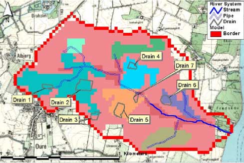
Figure 3.10 Stream system in Lillebæk. Different drain areas are connected – these are marked with different colours. Drain 1-7 are small drain areas, where drainflow is measured.
Figur 3.10 Å-system i Lillebæk. Forskellige drænede områder er tilsluttet å-systemet, disse er vist med forskellige farver. Dræn 1-7 er små områder hvor drænafstrømning er målt.
For Odder Bæk, it was not expected that drains would be of importance. However, the appearance of clay deposits near the soil surface indicates a need for artificial drainage in particular in the areas close to the stream. An effort was therefore made to identify existing drainage systems. At present, 25 -30 known drainage systems have been identified, most of which are located in the area around Riskær and along the piped runoff from Gislum Enge. It is, however, most likely that more drainage systems are active, but as these have been established long time ago by the local farmers advisory service, data are only accessible if the name of the farmer owning the land at the time of establishment is known. At present it is therefore assumed in the model that all areas near the stream are artificially drained. The depth of the drains is 1 m.
Within Odder Bæk catchment, one drain station has been monitored with respect to water flow and solute transport. It was therefore assumed that these data could be used for detailed calibration of parts of the model. In addition, information of pesticide application on the fields assumed to feed the drain station has been obtained through interviews with farmers. These should have been used for a cause and effect analysis - how long time does it take from application to a pesticide is found in drain water. The drain is shown on Figure 3.11.
Unfortunately it appears that a much larger area than indicated on Figure 3.11 drain to station 51. In , the model has estimated the topographical catchment for the drain station. It shows that the water caught by the drained area stem from the green and red triangular areas to the west of stream. This has implications for the interpretation of pesticide findings in the drain water.
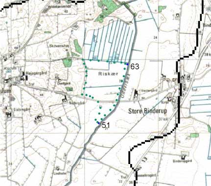
Figure 3.11 Location of the originally assumed drainage catchment and the drain station (51) in Odder bæk catchment. The assumed drainage area is delineated by the spots.
Figur 3.11 Placering af det forventede drænopland og drænstation (51) i Odder Bæk-oplandet. Drænoplandet er indrammet med prikker.
Model simulations based on the illustrated catchment area for the drain gave reasonable results during the winter season, but underestimated the flow during the summer season. This was not in accordance with the fact that groundwater measurements showed a falling water level during summer. The drainage system was investigated further and it became clear that side drains are found up to three meters from the stream at level with the bottom of the stream. Water may therefore, during the summer, move from the stream to the drain and back in the stream further down. Alternatively, there is an unidentified inflow from the north.
The conclusion is that the mass balance with respect to solutes on this drain is very doubtful and that the drain is not suited for validation of pesticide simulations.
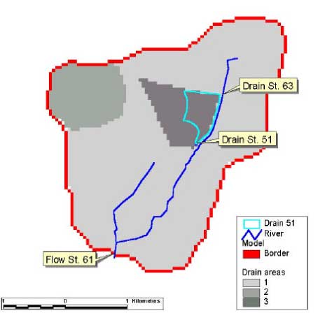
Figure 3.12 Drainage zones for different parts of the stream system. Note the estimated catchment for stream station 63 is the whole area upstream the station and the area for station 51 (dark gray) is larger than the actual pipe-drained area, indicated with a line.
Figur 3.12 Drænzoner for forskellige dele af å-systemet. Bemærk at det estimerede opland for å-station 63 er hele arealet opstrøms for stationen, og arealet til station 51 (mørkegrå) er større end det rør-drænede område, der er indikeret med en linie.
3.1.8 Abstraction
For Lillebæk, abstraction data from the County of Funen has been applied for the waterworks of Oure. On average, the yearly abstraction is approximately 100000 m3 influencing the overall water balance of the Lillebæk catchment significantly. Other individual water abstractions are present in the area, but none of them exceeds 3000 m3/year, which is found to be of local interest only.
In Figure 3.13 the four production wells of the waterworks of Oure are shown. It is seen that the screen of three of the wells is located in the lower primary aquifer whereas the screen of the last well is located in the upper secondary aquifer. During 1999-2000 BAM contamination has been monitored in two of the wells in the primary aquifer.
Figur 3.13 Vandforsyningsboringer tilhørende Oure vandværk. Filtersætningen i brøndene er vist med blå og vandspejlet med de trekantede markører.
Abstraction data were received from the county of Northern Jutland. Figure 3.14 shows the location of the wells. The total amount extracted from the Gislum Waterworks is constantly about 6.000 m3 per year, while extraction for irrigation differs from year to year – from almost nothing in year 1999 to 18.500 m3 in year 1992.
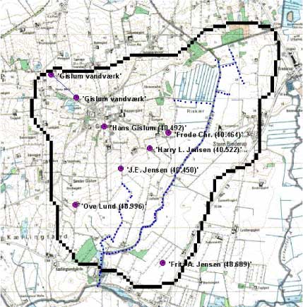
Figure 3.14 Water supply wells and irrigation wells located in the Odder Bæk catchment.
Figur 3.14 Placeringen af vandforsyningsbrønde og vandingsbrønde i Odder Bæk-oplandet.
3.2 Modelling water flow in the stream models
3.2.1 Cross-sections
The spatial discretion of the stream model is based on a series of cross-sections. Linear interpolation was conducted between these to define the calculation unit of the MIKE 11 model. To obtain an updated and detailed description of the geometry of the streams, measurement of the cross- sections conducted in the winter of year 1999 to 2000. The measured cross- sections were combined with existing information of cross-sections of the counties and a final cross section-data base was established for each set up of MIKE 11. The distance between the cross-sections depends on the uniformity of the stream and on the logistic constraints, such as the impossibility of measuring cross-sections in the dense forest of the catchment of Lillebæk. Hence the distance between the cross-sections varies between hundreds of meters at the most uniform sections of Odder Bæk to a few meters around bridges or other structures causing major local changes of the shape of the streams. An overview of the horizontal placement of the cross-sections in Lillebæk and Odder Bæk appear from Figure 3.15 and Figure 3.16 respectively, whereas the code of the bottom of the creek of each cross-section appears from Figure 3.17 and Figure 3.18 respectively.
Figure 3.15 Horizontal distribution of the cross-sections of the MIKE 11 model in the Lillebæk catchment
Figur 3.15 Horizontal fordeling af tværsnit i MIKE 11-modellen for Lillebæk-oplandet.
Figure 3.16 Horizontal distribution of the cross-sections of the MIKE 11 model in the Odder bæk catchment
Figur 3.16 Horizontal fordeling af tværsnit i MIKE 11-modellen for Odder Bæk-oplandet.
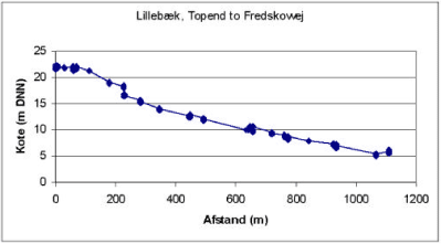
Figure 3.17 Altitude of the cross-sections of the MIKE 11 model in the Lillebæk catchment.
Figur 3.17 Kote for de i MIKE 11-modellen anvendte tværsnit fra Lillebæk-oplandet.
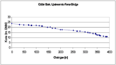
Figure 3.18 Altitude of the cross-sections of the MIKE 11 model in the Odder bæk catchment.
Figur 3.18 Kote for de i MIKE 11-modellen anvendte tværsnit fra Odder Bæk-oplandet.
3.3 Pesticide model for the catchment
3.3.1 Spraying data
The counties of Funen and Northern Jutland supplied GIS-maps with field numbers for 1998-2000, with corresponding files of management practices and pesticide use. These files contain information regarding date of spraying and amount sprayed. The information for selected pesticides is transformed to input for MIKE SHE. The overall use of pesticide in Lillebæk and Odder Bæk is shown in Table 3.3 and Table 3.4.
Table 3.3 Area treated with selected pesticides in Lillebæk from 1998 to 2000. Note that the spraying season of 1998 starts during autumn 1997.
Tabel 3.3 Areal behandlet med udvalgte pesticider i Lillebæk fra 1998 til 2000. Bemærk at sprøjtesæsonen 1998 begynder i efteråret 1997.
| 1998 | 1999 | 2000 | ||||
| Pesticide | ha | kg | ha | Kg | ha | kg |
| Bentazon | 17 | 3.7 | 7 | 2.2 | 6 | 4.2 |
| Pendimethalin | 148 | 57.8 | 24 | 9.5 | 267 | 135.6 |
| Fenpropimorph | 542 | 62.3 | 264 | 30.0 | 200 | 20.1 |
| Ioxynil | 165 | 12.9 | 248 | 18.6 | 190 | 13.7 |
| Ethofumesat | 31 | 3.4 | 35 | 3.9 | 56 | 6.3 |
| Isoproturon | 167 | 115.9 | 10 | 3.6 | 183 | 127.8 |
| Terbutylazin | 19 | 6.4 | 9 | 5.9 | 8 | 6.1 |
| Diuron | 2 | 1.2 | 1 | 1.0 | 16 | 16.9 |
| Pirimicarb | 116 | 7.5 | 93 | 8.9 | 98 | 6.7 |
| Prochloraz | 0 | 0.0 | 4 | 0.2 | 0 | 0.0 |
| Propiconazol | 456 | 17.8 | 233 | 9.2 | 109 | 4.5 |
* The sprayed area inside the catchment is only approximately 10 ha, as parts of the fields are outside the catchment. aTreated area overestimated as some of the fields included in the calculation are not located within the model catchment area. As a result of this the amounts may not represent exactly what is being applied within the model catchment.
Table 3.4 Area treated with selected pesticides in Odder Bæk from 1998 to 2000. Note that the spraying season of 1998 starts during autumn 1997.
Tabel 3.4 Areal behandlet med udvalgte pesticider i Odder Bæk fra 1998-2000. Bemærk at sprøjtesæsonen 1998 begynder i efteråret 1997.
| 1998 | 1999 | 2000 | ||||
| Pesticide | Ha | kg | ha | kg | ha | kg |
| Bentazon | 125 | 42.0 | 127 | 28.7 | 119 | 35.4 |
| Ethofumesat | 134 | 11.5 | 201 | 20.2 | 83 | 9.0 |
| Fenpropimorph | 185 | 24.3 | 245 | 27.4 | 224 | 24.4 |
| Ioxynil | 165 | 11.9 | 256 | 20.1 | 279 | 19.1 |
| Isoproturon | 94 | 44.1 | 116 | 53.7 | 116 | 25.0 |
| Pendimethalin | 165 | 97.5 | 222 | 102.2 | 213 | 114.0 |
| Terbutylazin | 61 | 29.9 | 72 | 23.0 | 10 | 2.6 |
| Diuron | 0 | 0.0 | 0 | 0.0 | 0 | 0.0 |
| Pirimicarb | 47 | 5.7 | 21 | 2.1 | 0 | 0.0 |
| Prochloraz | 21 | 0.5 | 0 | 0.0 | 21 | 4.8 |
| Propiconazol | 160 | 7.3 | 217 | 8.7 | 229 | 7.6 |
a Treated area overestimated as some of the fields included in the calculation are not located within the model catchment area. As a result of this the amounts may not represent exactly what is being applied within the model catchment.
3.3.2 Pesticide properties
The properties of the pesticides to be used for the simulation were extracted from the PATE database of the Danish Environmental Protection Agency. The treatment of the data turned out to be rather difficult as much of the data did not contain all the necessary information to transform the values to reference conditions. As part of the supporting information is confidential, the detailed calculations cannot be shown for most of the pesticides. However, the method used for normalisation of degradation values followed the guidelines given in FOCUS 2000.
The values used for modelling are given in Table 3.5.
Table 3.5 Pesticide properties extracted from the PATE database (Danish Environmental Protection Agency). The values (Halflife (DT50), sorption coefficient (Koc) and the Freundlich Exponent (1/n) are aggregated and normalised as described in FOCUS (2000). Not all data in the database could be normalised due to lack of information, and is therefore not included in the estimates.
Tabel 3.5 Pesticidegenskaber udtrukket af PATE-databasen (Miljøstyrelsen). Værdierne (Halveringstid (DT50), sorptionskoefficient (Koc) og Freundlich-eksponenten (1/n) er aggregeret og normaliseret som beskrevet i FOCUS (2000). Ikke alle data i databasen kunne normaliseres på grund af manglende information, disse er ikke inkluderet i estimaterne.
| Pesticide | DT50*, days | KOC ** | 1/n | Comments |
| Bentazon | 25.2 | 19.6 | both linear and freundlich adsorption among the results | |
| Pendimethalin | 66.3 | 15615 | 0.9¤ | It is stated in he data that adsorption follows a Freundlich isotherm, but no exponent is given. Degradation data results in a change in rate of 1.66 per 10 degrees (beta =0.0505) |
| Fenpropimorph | 22 | 4384 | Limited information, particularly on degradation | |
| Ioxynil | 1.86 | 236 | ||
| Ethofumesat | (45)& | 82.8 | The degradation data cannot be recalculated to reference conditions. | |
| Prochloraz | not collected | |||
| Isoproturon | 16.1# | 125 | 0.9¤ | It is stated in he data that adsorption follows a Freundlich isotherm, but no exponent is given. |
| Terbutylazin | 78.2 | 250 | 0.91¤ | A Q10-value of 3.43 was calculated from the values in the database. |
* The halflife is normalised to pF 2 and 20 degrees.
** For the freundlich values, KOC is determined at a concentration of 1 mg/l.
¤ In Odder Bæk, linear sorption was employed.
# Only two soils were included in the estimate from the PATE database. The dataset was extended with one soil from Lindhardt (1997). The extreme value was selected.
& No figure ws available for in the PATE database for DT50. A figure from the inception report (DHI et al., 1998) has been used.
3.3.3 Organic matter
In principle, the organic matter content of each of the known soil horizons should be used as input to the model. This is done in Lillebæk. However, for Odder Bæk, the soil types were modified compared to the original data, and no data existed for the organic soil. The values deduced are given in Annex B for each soil in the two catchments. Kd is then calculated as fOC * KOC. For Odder Bæk the foc-value are rather high and during the calibration phase, all values were halved in order to arrive at reasonable correspondence with observations.
3.3.4 Standard values
The default values for the FOCUS (2000) report were used for the following parameters as a starting point:
- The diffusion coefficient in water is 4.3 x 10⁻⁵ m2/day. This value is generally valid for molecules with a molecular mass of 200-250.
- Dispersion length is set to 5 cm.
- If nothing else is known, the Q10-factor is 2.2 (change in degradation rate with 10 degrees change in temperature).
- The exponent of the Walker equation, relating the degradation to soil moisture (f = (θ/θref)B, Walker, 1974), is 0.7.
- The degradation depth is supposed to decrease with depth. From 30-60 cm, the value is multiplied with 0.5 and from 60-100 cm with 0.3. Below 100 cm, no degradation is expected to take place. This assumption, however, turned out to be too conservative compared to observations and the factor of 0.3 was extended downwards into the upper part of the groundwater.
- If no data are available, and a Freundlich relation is expected, the default value for the exponent is 0.9. However, data available in the Pate database with the EPA only in one case supported the use of a Freundlich exponent. In addition, the concentration range in which these values are established is different from the concentration range found in at least the lower part of the soil profile.
- The transpiration stream concentration factor is set to 0 for non-systemic compounds and to 0.5 for systemic compounds.
- The interception factor by leaves is estimated on the basis of the plant cover at the time of spraying. The basic curves used to estimate this are shown in Styczen et al. (2004b, Appendix 2). The values stem from Jensen and Spliid (2003) or FOCUS (2000), depending on crop.
3.4 Pesticide model for streams and ponds
3.4.1 Solar insolation
To describe the photolytic degradation of pesticides, measurements of intensity (global radiation) and the spectral composition of the solar insulation is required. The global radiation data used was measured data for Hornum (st. no. 20501), which was considered to be representative for normal Danish conditions. The composition of the solar insulation was calculated from data given in OECD (1995). Average values for the four seasons (spring, summer, autumn, winter) are used.
3.4.2 Dispersion
For Lillebæk and Odder Bæk a constant dispersion coefficient of 3 m2s-1, typical of small Danish streams, was used (DHI, 1997).
3.4.3 Suspended matter, temperature and pH
Measurements of the temperature and pH from Lillebæk and Odder Bæk was obtained from the councils of Funen and North Jutland respectively. For pH the average values of 7.6 for the years of 1995 to 2000 was used. For temperature time series of daily measurements conducted at daytime between 10 am to 2 pm were used. In Lillebæk the measurements was conducted at Fredskovvej, whereas the measurement at Odder Bæk was conducted at station 61 at the Farsø Bridge.
Suspended matter was added to the stream model (MIKE11) from the catchment model as the flow of particles through macropores.
3.4.4 Biomass of macrophytes
Ideally, the biomass of the macrophytes should have been background data for the set up of the model, but quantitative data for macrophytes was not available for any of the streams. The biomass of macrophytes was therefore estimated on the basis of information from the literature (Jensen and Lindegaard 1996) of the yearly succession in the biomass of macrophytes in Danish streams not covered by forest Figure 3.19.
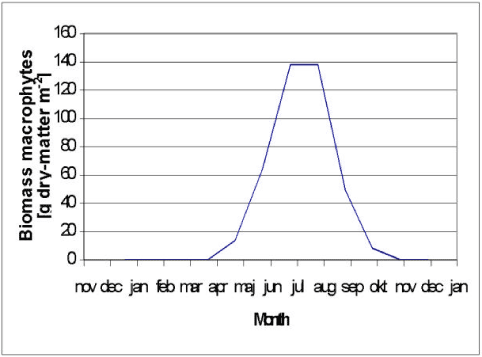
Figure 3.19 Biomass of macrophytes in light open danish streams.
Figur 3.19 Biomasse af makrofyter i lys-åbne Danske vandløb.
Based on the biomass of macrophytes was calculated assuming a forest cover of 50% for Lillebæk and 0% for Odder Bæk and an average depth of 0.1 m and 0.5 m for Lillebæk and Odder Bæk respectively.
3.4.5 Sediment bed
The diffusion into the sediment bed is heavily dependent on the size of the effective diffusion coefficient (Mogensen et al., 2004). On the basis of the calibration of the pond model against data for the experiments with artificial ponds (Helweg et al., 2003) an effective diffusion coefficient is determined and used for the sediment bed in ponds. For the stream a diffusion coefficient of 1.8 x 10⁻⁶ m2 h-1 corresponding to the molecular diffusion coefficient for a compound of a weight of 300 g mol-1 (Schwarzenbach, 1993) was used.
3.4.6 Sorption to sediment and suspended matter
For the compounds of Ioxynil, Bentazon and Pendimetelin, Kd, Koc, sorption and desorption rates were delivered by sub project 5 (Helweg et al., 2003). For the remaining compounds desorption rates was calculated from the Kd value as described in (Styczen et al., 2004b). Hence it is assumed that the ratio between the sorption and desorption rates is given by the Kd value and that sorption rate is compound independent and therefore similar to the sorption rate estimated for the above compounds. The validity of this assumption is further discussed by (Styczen et al., 2004b).
In case a Kd value was unavailable a Kd value was calculate either from the Koc or a Kow value for the pesticide and the organic content of the sediment/suspended matter as described by Styczen et al. (2004c). In every case the Kd, Koc or Kow values were extracted from a database, PATE, containing the data available for the EPA in connection with an approval procedure.
3.4.7 Sorption to macrophytes
Data for sorption to macrophytes are not available from the data delivered to the Danish EPA in connection with an approval procedure or from the PATE data base. The Kd values was therefore determined from the water solubility using adapted from Crum et al., (2000):
log(Kd) = 3.2 – 0.65 log(S), (Eq. 3.1)
where
S denotes the water solubility (mg/l).
Subsequently the kinetic of the sorption was determined from the Kd value as described for the sorption to particles (section 3.4.6).
3.4.8 Biological degradation in pore water and water column
On the basis of the biodegradation and sorption experiments of Helweg et al. (2003) a relative microbial activity of the free living bacteria and of the bacteria attacked to particles was calculated. Thereafter a total degradation rate and the particle concentration at which the degradation rate was determined were extracted from the data base PATE and the degradation rates of the dissolved pesticide in the pore water and in the water column was calculated as described by (Helweg et al., 2003).
3.4.9 Biological degradation at macrophytes
Data for biodegradation on macrophytes is not available from the data available to the EPA in connection with an approval procedure. In addition an approach for calculation of the biodegradation on macrophytes is not available from the literature. It was therefore decided not to include degradation on macrophytes in the model. The implication thereof is considered in the discussion.
4 Calibration and Validation of Water Flow
Calibration is performed in a number of steps – one concerning the water flow and one concerning the pesticide transport. Calibration of the water flow was done stepwise too – on the stream flow, on the groundwater flow and on the drain flow separately, and on the integrated system.
4.1 Data for calibration
For calibration of the water flow, the main sources of information are drain runoff, stream runoff and groundwater levels measured in the two catchments. For calibration of the pesticide transport, the main source of information is concentrations measured at drain stations.
As mentioned in Section 1.1, stream flow is measured at two stations, drain flow at 6 stations and head elevation at 15 wells in Lillebæk. Pesticide is measured at drain 2 and 6, and at the two flow stations (see Figure 4.1). The locations of the observation wells have during the calibration been a somewhat uncertain. Latest locations are used in the report and calculation of calibration statistics – some of these updates are done on basis of re-measuring the locations using GPS.
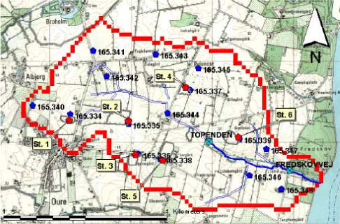
Figure 4.1 Location of measurement stations in Lillebæk - head elevation wells (blue petagons), flow measurement stations (crossed squares) and drainflow stations (St. 1-6).
Figure 4.1 Placering af målestationer i Lillebæk – pejleboringer (blå femkanter, afstrømningsmålere (firkanter med kryds) og drænafstrømnings-stationer (St. 1-6).
In Odder Bæk, stream flow is also measured at 3 stations, drain flow at one station and head elevation is measured in 17 groundwater wells, see Figure 4.2. The intermediate flow station was only active for at few years. Pesticide is measured in drain 51 and at the downstream station.
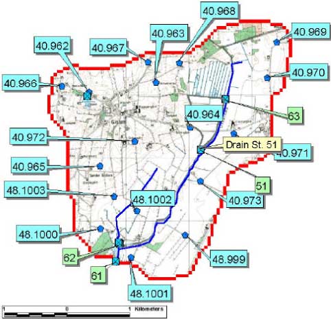
Figure 4.2 Location of measurements in Odder bæk - head elevation wells (blue petagons), flow measurement stations (crossed squares) and drainflow station (51).
Figur 4.2 Placering af målestationer i Odder Bæk – oplandet – pejleboringer (blå femkanter, afstrømningsmålere (firkanter med kryds) og drænafstrømningsstation (51).
Measurements of water generally cover the period from 1989 till 2000. Pesticide measurements were only carried out in 1999 and 2000 (end September).
The pesticide measurements are described by Iversen et al. (2003).
4.2 Calibration of water flow
4.2.1 Initial calibration of the MIKE 11 HD model
Before integration of the stream model (MIKE 11) into the catchment model, calibrations of the hydraulics was conducted. Calibration was performed for the period between 1989 to 1998. Measurements of discharge and water levels were use in the calibration. To take into account the water that enters the streams from the sides the difference between the water flow at the upstream and down stream stations was calculated and added as separate sources distributed evenly along the course of the streams.
For Lillebæk data from the stream stations shown on Figure 4.1 was used – i.e. discharge at the stream station at Fredskovvej and Topenden, and calibration was done on the water level at Fredskovvej.
For Odder Bæk, a similar calibration was conducted on the basis of measurements of discharge at stream station 61 and 63 and water levels at the stream station 61, see Figure 4.2.
4.2.2 Calibration of the MIKE SHE model
A proposed procedure for calibration/validation was described in the first status report of the project (DHI et al., 2000e). This procedure has been followed. However, soil moisture data were not used in the calibration.
Calibration was carried out as a split-sample – using part of the period for actual calibration and part of the period for validation. The actual calibration was done using trial and error procedure where each calibration simulation has been evaluated by statistical measures (mean error and root mean square). Calibration has been performed on different scales – mainly on catchment scale but also on drain catchment scale and single column scale.
On catchment scale the main parameters subject to calibration have mainly been the conductivities in the saturated zone, the leakage coefficient between the stream and the groundwater, and the drainage coefficient. The drainage coefficient is one of the main processes in both areas, however described by the least physical parameters. Besides, the exact location of the drain is somewhat uncertain. The measured stream flow and the groundwater levels have been the targets for the calibration.
Also the depth of the drains has been subject to calibration. The target for these calibrations has been the measured drain outflow. Results from the drain studies have been applied to the catchment models.
Soil properties have been subject to very restricted calibration. The field data and corresponding parameter estimations have provided the limitations for the values tried. The effect of different crops and soil types has been examined using the groundwater level as target. Results from the soil column calibrations are very uncertain due to boundary effects. The results have been test on catchment scale before they were applied.
In addition, simulations with the Daisy model were performed to test the general transport parameters selected for the soil profile. The test substance was nitrate. This exercise is not reported in detail, as it is only indicative for the pesticide modelling, and because several N-related factors have to be parameterised, which are not relevant for pesticide modelling anyway. However, for Lillebæk, the simulated and modelled nitrate fluxes were in good correspondence, and the setup has been handed over to the county of Funen and NERI. For Odder Bæk, the exercise is less interesting as the soil profiles required modifications to be used in the catchment model, and they are thus not directly comparable.
4.2.2.1 Lillebæk
Simulated and measured flow for the two stream stations in Lillebæk is shown in Figure 4.3. The dynamics of the flow is considered well described, and the error of the overall water balance is 3% only at the downstream end.
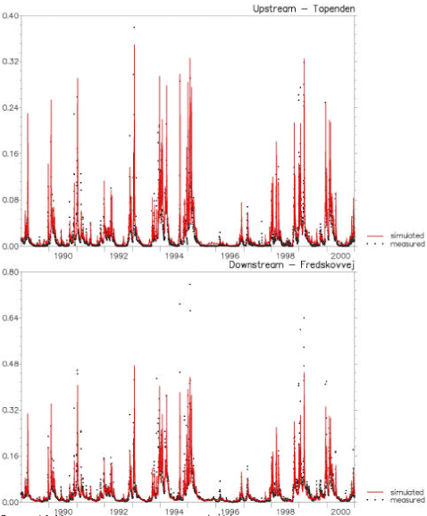
Figure 4.3 Measured and simulated flow (m3/s) in the upstream and downstream stream station in Lillebæk catchment.
Figur 4.3 Målt og simuleret afstrømning (m3/s) i den opstrøms og nedstrøms målestation i Lillebæk-oplandet.
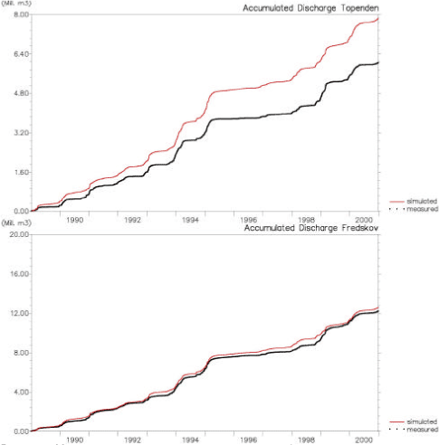
Figure 4.4 Measured and simulated accumulated flow in Lillebæk at the two stream stations.
Figur 4.4 Målt og simuleret akkumuleret afstrømning i Lillebæk ved de to afstrømningsmålestationer.
At the upstream station, the water balance error is 30%, mainly due to too much simulated flow during summer and additional discrepancy in 1995. Some of this uncertainty may be due to uncertainty regarding exactly where different drain systems are connected to the stream. Besides, the boundary conditions on the southern border in the sand lens are somewhat uncertain. Further field investigation is likely to reveal whether groundwater flow in the lens is towards the Hammersbro Bæk or Lillebæk – in other words, the location of the groundwater divide in the area influences the modelling.
Simulated and observed groundwater potentials in 15 wells is shown in Figure 4.5 - Figure 4.8. All values are related to the top layer – though it seems at little odd that the filter is placed in the clay rather than in the white sand layer.
In general there is at good match between the simulated and observed levels. In a majority of the wells there is a good match with the dynamics. Three wells are found to match neither the dynamics nor the level. Unfortunately these are all placed in the southern quadrant, see Figure 4.7. Modifications of the boundary conditions of the sand lens had good effect on calibration of these wells – however, with the given geological model it was not possible to lower the potential head on the boundary further.
Calibration on the period of 1989 to 1992 and the evaluation was done on statistical measures, mean error and root mean square error, standard deviation and Nash-Sutcliffe coefficient. The statistical measures are listed in Tabel 4.1, both for the calibration period the following validation and the total period 1989 to 2000.
For the groundwater level, the mean error, the root mean square error and the standard deviation on the residuals were used – using the equations listed below, where the following symbols are used:
Oi = Value of observation no. i
Pi = Value of prediction no. i
N = Number of observations
Mean error
![]()
Root mean square error
![]()
Standard deviation
![]()
For the river flow the evaluation measures used are the mean error, the root mean square error and the Nash-Sutcliffe coefficient. This coefficient investigates whether it is better to look at the average value of the measurements than at the model predictions. The interval of NS is ]-∞;1].
Nash-Sutcliffe coefficient
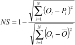
Table 4.1 Statistical measures on match between observed and simulated flow and groundwater level in Lillebæk. Values for calibration, validation and total period.
Tabel 4.1 Statistiske mål på overensstemmelsen mellem observeret og simuleret afstrømning og grundvandsniveau i Lillebæk. Værdier for kalibreringen, valideringen og den totale periode.
| Obs. ID | Calibration 1989-1992 | Validation 1993-2000 | Whole 1989-2000 | ||||||
| ME [m3/s] |
RMSE [m3/s] |
NS [-] |
ME [m3/s] |
RMSE [m3/s] |
NS [-] |
ME [m3/s] |
RMSE [m3/s] |
NS [-] |
|
| Fredskov | -0.0003 | 0.0210 | 0.7091 | -0.0022 | 0.0302 | 0.7128 | -0.0018 | 0.0273 | 0.7124 |
| Topenden | -0.0029 | 0.0118 | 0.7449 | -0.0057 | 0.0171 | 0.7171 | -0.0048 | 0.0154 | 0.7258 |
| Average | -0.0016 | 0.0164 | 0.7270 | -0.0040 | 0.0237 | 0.7150 | -0.0033 | 0.0214 | 0.7191 |
| ME [m] |
RMSE [m] |
STD [m] |
ME [m] |
RMSE [m] |
STD [m] |
ME [m] |
RMSE [m] |
STD [m] |
|
| 165.334 | 0.62 | 0.84 | 0.58 | 0.39 | 1.01 | 0.93 | 0.40 | 1.00 | 0.92 |
| 165.335 | 0.74 | 0.82 | 0.34 | 0.35 | 0.56 | 0.44 | 0.36 | 0.57 | 0.45 |
| 165.336 | -1.44 | 1.47 | 0.30 | -1.36 | 1.63 | 0.90 | -1.36 | 1.63 | 0.88 |
| 165.337 | 1.01 | 1.35 | 0.90 | 0.66 | 1.07 | 0.84 | 0.67 | 1.08 | 0.85 |
| 165.338 | -5.04 | 5.26 | 1.51 | -5.06 | 5.18 | 1.11 | -5.06 | 5.18 | 1.13 |
| 165.339 | -0.69 | 0.79 | 0.37 | -1.06 | 1.10 | 0.29 | -1.04 | 1.09 | 0.30 |
| 165.340 | 2.60 | 2.66 | 0.57 | 2.31 | 2.47 | 0.87 | 2.42 | 2.55 | 0.78 |
| 165.341 | 0.70 | 0.89 | 0.54 | 0.64 | 1.15 | 0.96 | 0.66 | 1.07 | 0.84 |
| 165.342 | -0.25 | 0.60 | 0.55 | -0.52 | 0.95 | 0.80 | -0.41 | 0.83 | 0.72 |
| 165.343 | -0.21 | 0.35 | 0.28 | -0.10 | 0.45 | 0.44 | -0.14 | 0.41 | 0.38 |
| 165.344 | -2.40 | 2.45 | 0.52 | -2.71 | 2.79 | 0.66 | -2.55 | 2.63 | 0.61 |
| 165.345 | 1.55 | 1.73 | 0.77 | 1.45 | 1.63 | 0.74 | 1.49 | 1.67 | 0.76 |
| 165.346 | -0.22 | 0.29 | 0.20 | -0.45 | 0.62 | 0.43 | -0.36 | 0.51 | 0.37 |
| 165.347 | -0.37 | 0.42 | 0.19 | -0.54 | 0.60 | 0.26 | -0.47 | 0.53 | 0.25 |
| 165.348 | -1.19 | 1.22 | 0.27 | -0.87 | 1.18 | 0.79 | -0.99 | 1.19 | 0.67 |
| Average | -0.31 | 1.41 | 0.53 | -0.46 | 1.49 | 0.70 | -0.43 | 1.46 | 0.66 |
Is that excellent, good or just acceptable? Early in the project an attempt was made to set limits for this (reported in DHI et al., 2000e). However, the limits were set on a rather arbitrary basis. Recently a guide to groundwater modelling has been published in Danish (Ståbi i grundvandsmodellering, GEUS, Henriksen et al. (red) (2000)), also considering issues on performance criteria. For the groundwater level, criterions are depending on the overall difference in measured groundwater table throughout the area – 5% for the ME and 10% for the RMSE for an excellent model.
Having a groundwater level in the area between 8 and 50 meters the criterion is 2.1 meter and 4.2 meter to the ME and RMSE, respectively. On the average this is clearly fulfilled, and only a few wells do not meet the demands.
For the river flow the criterion is less clear – however from examples in the guide the criterion were that if the median flow is less than 0.05 m3/s the deviation can be set to 100% on the ME and 200% on the RMSE. These values give a criterion of 0.03 m3/s on the ME and 0.06 m3/s on the RMSE – the model meets both.
The standard deviation and the Nash-Sutcliffe are not considered in the guide to groundwater modelling – however, some limits were suggested in DHI e al., 2000e.
For the standard deviation on the groundwater level residuals the criterion to an excellent, good or acceptable model in status report 1 is – 0.25 m, 0.40 m and 0.50 m respectively. None of these are meet on the average and only a few wells meet the criterion of an excellent model. It is clear, however, that the criteria are considerably stricter than what is specified in the Danish guidelines, and probably unrealistic.
For the Nash-Sutcliffe coefficient for the river flow the criterion is – 0.9, 0.8 and 0.7 for an excellent, good and acceptable model respectively. The Nash-Sutcliffe coefficient was in status report called R2 – here it is named NS (see Table 4.1). Here the model ranges as acceptable.
The conclusion is that compared to the recent groundwater modelling guide, the model ranges as excellent, while compared to the very ambitious (and probably unrealistic) goals set earlier in the project, the model only just reaches acceptable.
Figure 4.5 Measured and simulated groundwater potential in wells located in the northern quadrant of the Lillebæk catchment. The location of the wells are shown in Figure 4.1.
Figur 4.5 Målt og simuleret grundvandspotentiale i brønde i den nordlige kvadrant af Lillebæk-oplandet. Brøndenes placering er vist i Figur 4.1.
Figure 4.6 Measured and simulated groundwater potential in wells located in the eastern quadrant of the Lillebæk catchment. The location of the wells are shown in Figure 4.1.
Figur 4.6 Målt og simuleret grundvandspotentiale i brønde i den østlige kvadrant af Lillebæk-oplandet. Brøndenes placering er vist i Figur 4.1.
Figure 4.7 Measured and simulated groundwater potential in wells located in the southern quadrant of the Lillebæk catchment. The location of the wells are shown in Figure 4.1.
Figur 4.7 Målt og simuleret grundvandspotentiale i brønde i den sydlige kvadrant af Lillebæk-oplandet. Brøndenes placering er vist i Figur 4.1.
Figure 4.8 Measured and simulated groundwater potential in wells located in the western quadrant of the Lillebæk catchment. The location of the wells are shown in Figure 4.1.
Figur 4.8 Målt og simuleret grundvandspotentiale i brønde i den vestlige kvadrant af Lillebæk-oplandet. Brøndenes placering er vist i Figur 4.1.
4.2.2.2 Odder Bæk
Simulated and measured flow for the upstream, downstream station, and the drain in Odder Bæk is shown in Figure 4.9. The average error on the downstream flow is 5% and 13% on the upstream flow. It is obvious, however, that the drain flow is poorly simulated during the summer period. As described in section 1.1.5, the catchment for the drain is much larger than anticipated at the start of the project. Furthermore, the drain is found in the same depth as the bottom of the stream and only 3 meters from the stream. The only explanation of the water in the drain during the summer is that water runs from the stream to the drain, as the groundwater is found at greater depth. The drain is therefore not suitable for pesticide calibration.
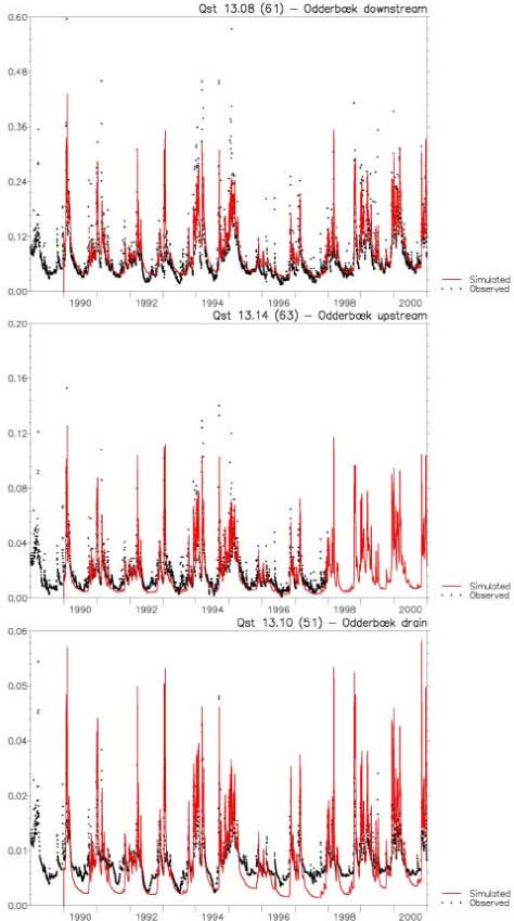
Figure 4.9 Measured and simulated flow (m3/s)at the downstream, at the upstream and at the drain station in Odder Bæk.
Figur 4.9 Målt og simuleret afstrømning (m3/s) ved den nedstrøms og den opstrøms afstrømningsstation og drænstationen i Odder Bæk.
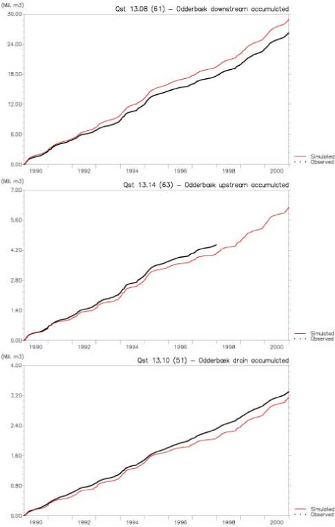
Figure 4.10 Measured and simulated accumulated flow at the downstream, at the upstream and at the drain station in Odder Bæk.
Figur 4.10 Målt og simuleret akkumuleret afstrømning ved den nedstrøms og opstrøms afstrømningsstation og drænstationen i Odder Bæk.
Simulated and observed groundwater potentials in 17 wells is shown in Figure 4.11. Values are related to the layer covering the filter.
In general the match between the simulated and observed levels is fair. In 11 of the well there is found a fair match on the dynamics. In 5 (40.962, 40.967, 40.968, 48.1000 and 48.999) out of the 11 wells the level is matched too – those wells are located in the northern and southern part of the model area. The most southern well (48.1001) is very close to the border – and here neither the dynamics nor the level is matched. The observations are placed above the applied surface topography. Also in the well between Odder Bæk and Gislum Enge the observations is found to be above the surface topography. In the eastern part the observations are matched on the levels but not on the dynamics.
Table 4.2 Statistical measures on match between observed and simulated flow and groundwater level in Odder Bæk. Values for calibration , validation and total period.
Tabel 4.2 Statistiske mål for overensstemmelsen mellem observeret og simuleret afstrømning og grundvandsniveau i Odder Bæk. Værdier er givet for kalibreringen, valideringen og den totale periode.
| Obs. ID | Calibration 1994-1996 | Validation 1996-2000 | Whole 1990-2000 | ||||||
| ME [m3/s] |
RMS [m3/s] |
NS [-] |
ME [m3/s] |
RMS [m3/s] |
NS [-] |
ME [m3/s] |
RMS [m3/s] |
NS [-] |
|
| Downstream | -0.0026 | 0.0417 | 0.63 | -0.0048 | 0.0361 | 0.45 | -0.0040 | 0.0394 | 0.51 |
| Upstream | 0.0022 | 0.0119 | 0.54 | 0.0030 | 0.0078 | 0.26 | 0.0023 | 0.0112 | 0.42 |
| Drain | 0.0068 | 0.0081 | -1.36 | 0.0063 | 0.0069 | -2.94 | 0.0066 | 0.0076 | -1.73 |
| Average | 0.0021 | 0.0206 | -0.06 | 0.0015 | 0.0169 | -0.74 | 0.0016 | 0.0194 | -0.27 |
| ME [m] |
RMS [m] |
STD [M] |
ME [m] |
RMS [m] |
STD [M] |
ME [m] |
RMS [m] |
STD [M] |
|
| 40.962 | -1.56 | 1.58 | 0.27 | -1.13 | 1.13 | 0.14 | -1.30 | 1.33 | 0.29 |
| 40.963 | -0.96 | 0.99 | 0.22 | -0.78 | 0.80 | 0.18 | -0.85 | 0.88 | 0.22 |
| 40.964 | -2.00 | 2.01 | 0.22 | -1.92 | 1.92 | 0.19 | -1.96 | 1.97 | 0.20 |
| 40.965 | -3.00 | 3.01 | 0.22 | -3.00 | 3.02 | 0.32 | -3.00 | 3.01 | 0.27 |
| 40.966 | 1.23 | 1.28 | 0.36 | no obs. | no obs. | no obs. | 1.23 | 1.28 | 0.36 |
| 40.967 | -0.05 | 0.16 | 0.15 | no obs. | no obs. | no obs. | -0.05 | 0.16 | 0.15 |
| 40.968 | 0.03 | 0.10 | 0.10 | 1.72 | 1.72 | 0.04 | 0.69 | 1.07 | 0.83 |
| 40.969 | 1.04 | 1.71 | 1.36 | no obs. | no obs. | no obs. | 1.04 | 1.71 | 1.36 |
| 40.970 | 0.15 | 0.50 | 0.47 | no obs. | no obs. | no obs. | 0.15 | 0.50 | 0.47 |
| 40.971 | -0.21 | 0.47 | 0.42 | no obs. | no obs. | no obs. | -0.21 | 0.47 | 0.42 |
| 40.972 | -2.02 | 2.05 | 0.38 | no obs. | no obs. | no obs. | -2.02 | 2.05 | 0.38 |
| 40.973 | 0.41 | 0.94 | 0.84 | no obs. | no obs. | no obs. | 0.41 | 0.94 | 0.84 |
| 48.999 | 0.15 | 0.35 | 0.32 | 0.26 | 0.37 | 0.26 | 0.23 | 0.37 | 0.30 |
| 48.1000 | 0.43 | 0.49 | 0.23 | 0.41 | 0.44 | 0.17 | 0.41 | 0.45 | 0.20 |
| 48.1001 | 3.07 | 3.07 | 0.21 | no obs. | no obs. | no obs. | 3.07 | 3.07 | 0.21 |
| 48.1002 | 2.07 | 2.09 | 0.27 | no obs. | no obs. | no obs. | 2.07 | 2.09 | 0.27 |
| 48.1003 | 0.20 | 0.35 | 0.29 | no obs. | no obs. | no obs. | 0.20 | 0.35 | 0.29 |
| Average | -0.06 | 1.24 | 0.37 | -0.64 | 1.34 | 0.18 | 0.01 | 1.28 | 0.42 |
The final calibration on the period of 1994 to 1996 and the evaluation of the model has been done using statistical measures, mean error and root mean square. The statistical measures are listed in Table 4.2, both for the calibration period, the following validation and the total period 1990 to 2000.
Using the guidelines – mentioned under the Lillebæk calibration – for setting the criterion to the ME, RMSE and STD for the groundwater level an excellent model fulfils the 1.0 m, 2.0 m and 0.25 m for the three statistical measures. A measured groundwater level span in the area from the lowest 15 meter to the highest 35 meter gives the criterion of 1 and 2 meters to the ME and RMSE, and the 0.25 m criterion to the STD is taken from DHI et al. (2000e).
The model complies with the performance criteria for an excellent model – except for the STD-criteria were the model can be characterised as a good model.
The average flow downstream is around 0.07 m3/s – between 0.05 and 0.1 m3/s. The recommended criterion is 50% and 100% – which gives a criterion to the ME and RMSE of 0.035 and 0.07 m3/s. The model meet these performance criteria.
For the STD the criterion taken from the 1st status report 0.7 for an acceptable model. Even disregarding the performance in the drain station will not give a model performance that can fulfil this criterion. The conclusion must be that the criteria set up earlier in the project were unrealistically strict.
Again the conclusion is that according to the guide on groundwater modelling, the model is excellent.
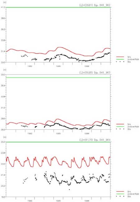
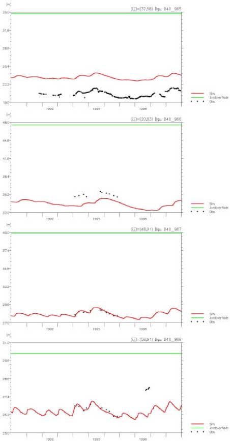
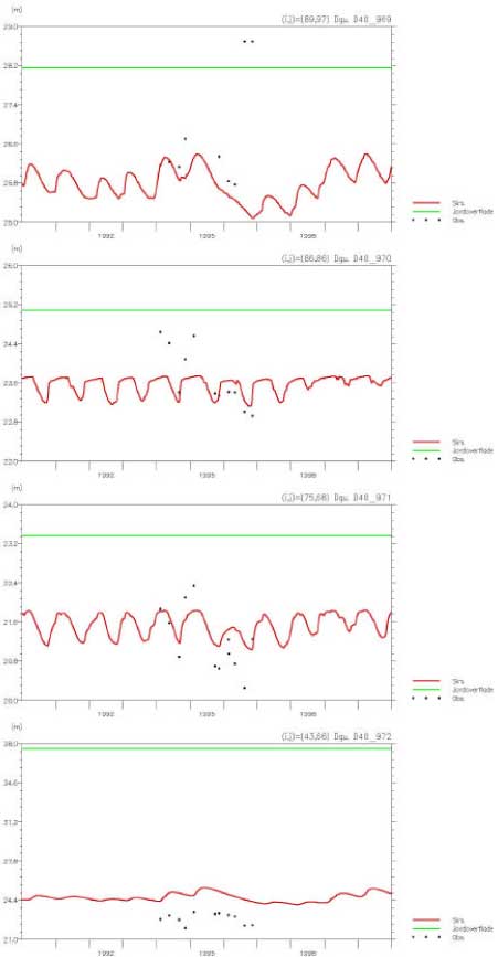
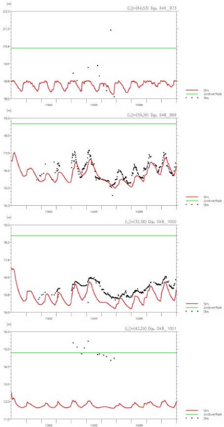
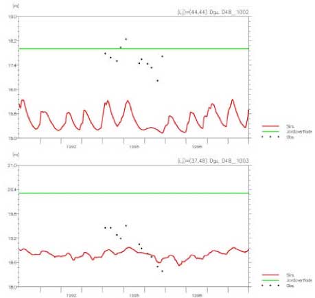
Figure 4.11 Measured and simulated groundwater potential in wells located in Odder bæk catchment.
Figur 4.11 Observeret og simuleret grundvandspotentiale i brønde i Odder Bæk-oplandet.
5 Calibration of Artificial Ponds
- 5.1 Calibration and validation
- 5.2 Process considered in the calibration
- 5.3 Calibration results
- 5.4 Verification of pesticide model for artificial ponds
- 5.5 Conclusion on the calibration and verification
5.1 Calibration and validation
A number of fate experiments with artificial ponds were conducted (Helweg et al., 2003). For details of the experimental procedures see Helweg et al., (2003). In brief the pesticides were applied as a single initial spraying event, where after the concentrations in the water column were measured for a period of up to 3 months. In addition a few measurements of the concentrations in the sediment were conducted.
For the compounds of Pendimethalin, Ioxynil and Bentazon biodegradation and sorption experiments were conducted by Helweg et al., (2003). Some of the experiments of Helweg et al., (2003) were conducted by sediment collected from the artificial ponds and the experiments might therefore be considered as dedicated experiments. It was therefore decided to conduct the calibration of the pond model on the basis of the artificial pond experiments with Ioxynil, Pendimethalin and Bentazon. Pond experiments with Glyphosate and Fenpropimorph was left for validation. Furthermore it was decided to use the experiments in ponds without macrophytes for validation, since these ponds was considered as different systems. Finally it was decided to use Ioxynil for validation purposes for reasons discussed below. An overview of the conducted experiments and the use of them is shown in Table 5.1.
Table 5.1 Overview of the experiments with artificial ponds used for calibration and verification of the pond model.
Tabel 5.1 Oversigt over eksperimenter udført med de kunstige vandhuller, anvendt til kaliberering og validering af vandhulsmodellen.
| Date for spraying | Compound | Init. conc. [μg/l] |
Used for | Remark |
| 9/6/1999 | Ioxynil | 1.4 | Verification | |
| 9/6/1999 | Bentazon | 1.49 | Calibration | |
| 7/9/1999 | Pendimethalin | 1.48 | Calibration | |
| 7/9/1999 | Fenpropimorph | 1.48 | Verification | |
| 9/5/2000 | Glyphosate | 9.64 | Verification | |
| 5/9/2000 | Pendimethalin | 2.15 | Calibration | |
| 5/9/2000 | Fenpropimorph | 2.15 | Verification | |
| 5/9/2000 | Pendimethalin | 2.15 | Verification | Macrophyte removed |
| 5/9/2000 | Fenpropimorph | 2.15 | Verification | Macrophyte removed |
5.2 Process considered in the calibration
To run the pond model more than 20 input parameters need to be specified. However, many of these are either solely defined by the physical and chemical properties of the pesticide (e.g. pKa or Henrys constant) or measured with high precision (e.g. water temperature and pH), making a consideration of such parameters irrelevant in connection with the calibration. Hence the calibration will focus of a few selected process or parameters, which not are readily determined by the available data. An overview of the process selected for the calibration is provided below.
5.2.1 Calibration of biodegradation in the sediment
An approach for calculation of biodegradation rates for the sediment compartment of the model on the basis of standardised laboratory test of biodegradation, which takes the high concentrations of particles in the sediment in to account, was developed by Helweg et al., (2003). Hence the approach takes in to account that particles on the one hand might decrease the bioavailability of the pesticides through sorption and on the other hand offers a significant substrate for bacteria.
In brief the approach rely on estimations of the number of active biodegrading bacteria per mass of sediment particles and the concentration of free living (pelagic) bacteria. Assuming that the number of bacteria per particle and the concentration off free living bacteria are constant the biodegradation of pesticides in the pore water can be calculated from a linear extrapolation of the biodegradation rates measured in the laboratory test to the sediment compartment of the models. However, the laboratory tests are conducted at particle concentrations in the order of 1000 gm-3, which is much lower than the particle concentrations of sediments. Hence the extrapolation involves a critical extrapolation from low to high concentrations of particles. For instance, the oxygen concentrations in the sediment might locally and temporary be much lower than the oxygen concentrations of the laboratory experiment, which might violate the assumption of linearity between the particle concentrations and the activity of the bacteria. In addition, the area of the sediment particles, which are in contact with the pore water, is lower in the sediment than in the shaking bottle experiment conducted by Helweg et al., (2003). A verification and possible adjustment of the approach of Helweg et al., (2003) is therefore an important task of the calibration of the model.
5.2.2 Calibration of the sorption to macrophytes
No data for the description of the sorption of the selected pesticides to macrophytes are available. The calibration of the sorption to macrophytes therefore has to be based on theoretical considerations. These theoretical considerations appear from Appendix C. In brief the considerations revealed that the uptake rate of pesticides through the surface (cuticle) and into the lumen of the leaves was in the order of 10-3 to 10-4 hour-1. Based on these fairly low rates it was thus decided to omit the uptake of pesticides in to the leaf from the description of the sorption of pesticides to macrophytes. Hence the sorption of pesticide to the macrophytes was assumed given by the sorption to the biofilm at the surface of the macrophytes. An important task of the calibration is thus to determine the concentration of algae and bacteria of the biofilm attacked to the surface of macrophytes.
Beforehand it was decided to investigate the performance of the model in the interval of 2.5 g-biofilm m-3 to 20 g-biofilm m-3. The lower value corresponding to an area cover of macrophytes of 25% percent and a concentration of microalgae of appr. 100 mg-chlorophyll Α m-2,which is a typical value for the concentration of benthic algae in Danish streams in the early spring, when the concentration of algae still is rather small (Sand-Jensen and Lindegaard 1996). The high value of 20 g-biofilm m-3 corresponds to, for instance, a macrophyte cover of 40% and a concentration of microalgae of appr. 400 mg-chlorophyll Α m-2, which is a typical value for the concentration of benthic algae in Danish streams in the summer, when the concentration of algae reach a maximum (Sand-Jensen and Lindegaard 1996).
5.2.3 Calibration of the photolysis
The coverage of macrophytes is important for the extent of the photolysis, since light is absorbed in the leaves of the macrophytes. A task for the calibration is therefore to determine the percentage area of the pond covered by macrophyte leaves absorbing the incoming light and thereby affecting the photolysis. It was decided to investigate the performance of the model in the interval of macrophyte coverage of 10 to 50% assuming that all the incoming light are absorbed in the macrophyte leaves.
Besides the absorption of light in the leaves of macrophytes a significant absorption might also take place in the water column itself, due to the presence of suspended and dissolved matter. Another task of the calibrations was thus to determine the light attenuation coefficient of the water column. For that purpose the performance of the model for attenuation coefficients in the interval of 0.5 to 2.5 m-1 was examined. An attenuation coefficient of 0.5 m-1 (base 10) corresponds to a secci depth of 8 m if it is assumed that:
- 10 percent of the incoming photosynthetic active (PAR) light remains at the secci depth,
- light attenuation at wavelengths of 300 nm is 4 times higher than the light attenuation in the photosynthetic active range (400 to 700 nm).
The later assumption is supported by adapted from Smith and Baker (1979). An attenuation coefficient of 2.5 m-1 corresponds to a secci depth of 1.6 m. Light attenuation at wavelengths of 300 nm is considered most relevant since the investigated pesticides have absorption maxima in this range.
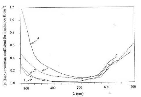
Figure 5.1 Diffuse attenuation coefficients as a function of wave length for different types of water bodies. Adapted from Garde 1998.
Figur 5.1 Diffuse lysudslukningskoefficient som funktion af bølgelængden for forskellige typer vand. Efter Garde 1998.
5.2.4 Calibration of the effective diffusion coefficient
An earlier model based study of the fate of Pyrethroids pesticides in the same artificial ponds as used in the present study revealed that diffusion and a subsequent sorption to sediment particles was among the most important process for the fate of hydrophobic pesticides (Mogensen et al., 2004). Furthermore, it was found that the apparent or effective diffusion coefficient was much higher than the molecular diffusion coefficient. One reason for this might be that the surface of the sediment is crude, which makes the effective area for diffusion much larger (see Mogensen et al., 2004 for further details).
An alternative or supplementary explanation of the high effective diffusion coefficients might be a local high concentration of organic matter in the upper part (< 1mm) of the sediment causing a higher sorption to particles. Hence, if the sorption to particles is estimated for a sample of the upper few cm of the sediment the content of organic matter might be underestimated, which causes an underestimation of the sorption for at least for hydrophobic pesticides with a high affinity for organic matter. It must be stated that the product of the sorption (retention) and the diffusion determine the overall sediment uptake caused by diffusion and subsequent sorption. An underestimated sorption might thus be compensated by a higher effective diffusion coefficient.
An effective diffusion coefficient for the artificial ponds of 1.3x10⁻⁴ m2h-1 was determined by Mogensen et al., (2004) using inverse modelling. However, this value seems to be specific for the experiments examined by Mogensen et al., (2004), since major differences in the disappearance rates for Fenpropimorph and Pendimethalin have been observed for the years of 1999 and 2000 (Helweg et al., 2003). The reasons for the different disappearance rates are discussed by Helweg et al., (2003) and might, among other things, involve differences in the extent of sorption of the pesticides to dissolved organic matter in the water column. Another or supplementary explanation might be differences in the extent of vertical mixing of the water column. However, data for a quantitative description of these phenomena are not available and descriptions of these phenomena where not considered when equations of the present model was described. As a consequence it is not possible to include the effect of dissolved organic matter and vertical mixing in the model. Consequently it was decided to determine an effective diffusion coefficient causing the best average fit of the artificial pond experiments conducted in 1999 and 2000 (Helweg et al., 2003).
As basis for this it was decided to examine the performance of the model when the diffusion coefficients was set to 1.5 x10⁻⁵, 5x10⁻⁵, 1.3x10⁻⁴ (the value of Mogensen et al., 2004), 5x10⁻⁴ and 1.5x10⁻³ m2h-1.
5.2.5 The quantitative importance of the different process
When calibrating a model one needs to consider that the importance of the different process is highly dependent on the physical and chemical properties of the pesticides. A framework for quantification of the relative importance of the different process for the outcome of the pond model on the basis of the physical and chemical properties are provided by the decisions trees in chapter 8 in Styczen et al., (2004b). To focus the calibration effort on the most relevant process, this framework was therefore applied to the pesticides selected for the calibration. The physical, chemical and biological properties of the pesticides appear from Table 5.2, whereas the results of the evaluation of the importance of the different process appear from Table 5.3.
The pesticide properties were extracted from PATE (the database of the EPA) and from chemical handbooks. The quality and quantity of the data for pesticides properties is thus assumed to resemble the quality of the data available for the EPA in connection with approval procedures in the future. Desorption rates were calculated from the Kd or Koc values assuming a constant sorption rate as recommended by Helweg et al., (2003). The gas and liquid exchange coefficient, used for calculation of evaporation, were estimated on the basis of Asman et al. (2003). The particle concentration in the water phase was set to 1 g m-3 and the sediment porosity was set to 0.75. The bulk dry density of the sediment was set to 0.5 kg/l. The pH of the pond was set to 7.6. The photolysis rates correspond to the rates in clear water at noon on a sunny summer day. Hence the actual degradation rate in the ponds will be lower due to attenuation of the light. For Bentazon and Ioxynil the photolysis was calculated on the basis of the quantum yield and the absorption spectra of Figure 5.2 to Figure 5.3.
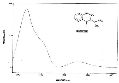
Figure 5.2 Absorption spectra for Bentazon adapted from Chiron et al. (1995).
Figur 5.2 Absorptionsspektrum for Bentazon, efter Chrion et al. (1995).
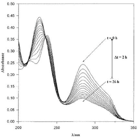
Figure 5.3 Absorption spectra of ioxynil adapted from Millet et al. (1998). The different curves reflect the degradation of ioxynil and hence decreased absorption with time.
Figur 5.3 Absorptionsspektrum for ioxynil, efter Millet et al. (1998). De forskellige kurver skyldes nedbrydningen af ioxynil og derfor nedsat absorption over tid.
In accordance with the framework for evaluation of the importance of the different process (Table 5.3), photolysis was the only process of importance for the fate of Bentazon, whereas photolysis and diffusion in to the sediment were of importance for ioxynil. It was therefore decided to use Bentazon for calibration of the photolysis and to leave ioxynil for validation.
Table 5.2 Pesticides properties used for the calibration. The values in brackets indicate the final values after the calibration have been finished.
Tabel 5.2 Pesticidegenskaber anvendt i kalibreringen. Værdierne i paranteser er de endelige værdier da kalibreringen var tilendebragt.
| Property | Compound | |||||
| Ioxynil | Pendimethalin | Bentazon | ||||
| Value | Reference | Value | Reference | Value | Reference | |
| Water solubility [gm-3] w.s. | 50 | Tomlin 1994 | 0.3 | Tomlin 1994 | 570 | Tomlin 1994 |
| Desorption [h-1] particles | 2.41 | Calculated from Kd | 1.24E-02 | Calculated from Kd | 11 | Calculated from Kd |
| Kmacrophyt [m3g-1] km |
1.2e-4 | Calculated from w.s. | 3.5e-3 | Calculated from w.s. | 2.5e-5 | Calculated from w.s. |
| Desorption [h-1] macrophytes | 2.3 | Calculated from Km | 8.3E-02 | Calculated from Km | 11 | Calculated from Km |
| Kd [m3g-1] | 2.83e-5 | Helweg et al., 2003 | 7E-4 | Helweg et al., 2003 | 3.3e-6 | Helweg et al., 2003 |
| Koc [m3g-1] | 3.6e-4 | Helweg et al., 2003 | 0.021 | Helweg et al., 2003 | 13 | Helweg et al., 2003 |
| Alk. Hydrolyse [h-1mol [H+] –1] | 0 | EPA data base | 0 | EPA data base | 0 | EPA data base |
| Acid Alk. Hydrolyse [h-1mol [OH-] –1] | 0 | EPA data base | 0 | EPA data base | 0 | EPA data base |
| Neutral Hydrolysis [h-1] | 0 | EPA data base | 0 | EPA data base | 0 | EPA data base |
| Pka | 3.96 | Danish EPA | 2.8 | Danish EPA | 3.3 | Pesticide Handbook |
| Bio_deg_water column [h-1] | 1.85e-5 | Helweg et al., 2003 | 0.015 | Helweg et al., 2003 | 0 | Helweg et al., 2003 |
| Bio_deg_pore_water [h-1] | 8.3e-2 (7e-4) |
Helweg et al., 2003 | 28 (0.4) |
Helweg et al., 2003 | 0 (0) |
Helweg et al., 2003 |
| Gas_exchange [mh-1] | 45 | Asman et al. 2003 | 45 | Asman et al. 2003 | 45 | Asman et al. 2003 |
| Liquid_exchange [mh-1] | 0.029 | Asman et al. 2003 | 0.029 | Asman et al. 2003 | 0.029 | Asman et al. 2003 |
| Henrys constant (-) | 2.25e-8 | EPA data base | 1.10E-09 | EPA data base | 2.91e-14 | EPA data base |
| Quantum Yield | 2.4e-3 | Chiron et al., 1995 | ---- | ------- | 1.7e-5 | Calculated from Millet et al., 1998 |
| Photolysis rate [h-1] | 0.3 | Chiron et al., 1995 | 1e-3 | Sanders, P. 1985 in EPA data base | 2.6e-1 | Millet et al., 1998 |
| Retention in sediment | 15 | Calculated from Kd | 350 | Calculated from Kd | 2.4 | Calculated from Kd |
Table 5.3 The most important process for the calibration of the pond model for ioxynil, Bentazon and pendimethalin. The process was selected on the basis of the pesticides properties of Table 5.2 and the decision trees of chapter 8 in Styczen et al., (2003).
Tabel 5.3 De vigtigste processer i kalibreringen af vandhulsmodellen for ioxynil, Bentazon og pendimethalin. Processerne er udvalgt på basis af pesticidegenskaberne i Tabel 5.2 og beslutningsstøttetræet i kapitel 8 i Styczen et al.,. (2004b).
| Pesticide | Selected process |
| Pendimethalin | Effective diffusion in to sediment Degradation in sediment |
| Ioxynil | Photolytic degradation Effective diffusion in to sediment |
| Bentazon | Photolytic degradation |
5.3 Calibration results
5.3.1 Pendimethalin
When the values for Pendimethalin of Table 5.2 were used as input parameters the results of Figure 5.4 was obtained.
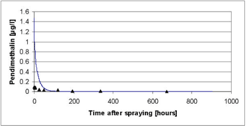
Figure 5.4 Simulated versus measured total concentration in the water column of pendimethalin for the artificial pond experiments of year 1999. The simulation was based on the data of Table 5.2 before modifications of the biodegradation and the diffusion in to the sediment as discussed in the text.
Figur 5.4 Observeret og simuleret totalkoncentration af pendimethalin i vandsøjlen for det kunstige vandhulseksperiment i 1999. Simuleringen er baseret på data fra tabel 5.2 før modifikation af bionedbrydningen og diffusion ind i sedimentet som diskuteret i teksten.
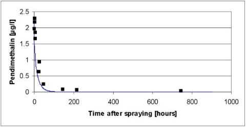
Figure 5.5 Simulated versus measured total concentration in the water column of pendimethalin for the artificial pond experiments of year 2000. The simulation was based on the data of Table 5.2 before modifications of the biodegradation and the diffusion in to the sediment as discussed in the text.
Figur 5.5 Observeret og simuleret totalkoncentration af pendimethalin i vandsøjlen for det kunstige vandhulseksperiment i 2000. Simuleringen er baseret på data fra tabel 5.2 før modifikation af bionedbrydningen og diffusion ind i sedimentet som diskuteret i teksten.
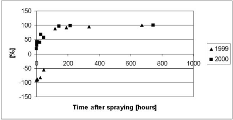
Figure 5.6 Residuals or relative difference between the simulated and measured total concentrations of pendimethalin in the water column of the experiments with artificial ponds in year 1999 and 2000. The simulations were based on the data of Table 5.2 prior to modifications discussed in the test.
Figur 5.6 Residualer eller relativ forskel mellem observeret og simuleret totalkoncentration af pendimethalin i vandsøjlen for det kunstige vandhulseksperiment i 1999 og 2000. Simuleringen er baseret på data fra tabel 5.2 før modifikationer som diskuteret i teksten.
As it appears from Figure 5.4 to Figure 5.6, the model severely underestimated the concentrations of pendimethalin in the water column after 100 hours both in year 1999 and 2000. In addition the concentrations before 100 hours were overestimated in year 1999. The underestimation after 100 hours was interpreted as an overestimation of a first order degradation rate whereas the overestimation before 100 hours in 1999 was interpreted as an underestimation of the effective diffusion coefficient.
According to Table 5.2 the most significant degradation takes place in the sediment and the procedure for extrapolation of biodegradation rates of Helveg et al., (2003) therefore seems to overestimate the biodegradation in the sediment. In an attempt to obtain a more appropriate fit of the model it was therefore decided to reduce the biodegradation in the sediment and to adjust the extrapolation procedure of Helveg et al., (2003) accordingly before the extrapolation procedure is implemented in the registration model (Styczen et al., 2004). In addition, it was decided to increase the effective diffusion coefficient of the sediment to avoid the severe overestimation in the first 100 hours after the spraying of pesticide in year 1999. After adjustments of the diffusion coefficient to 1.5 x 10⁻³ m2h-1 and the degradation rate in the sediment to 0.4 h-1 the results of Figure 5.7 to Figure 5.9 was obtained. The adjustments were found through successive changes of the degradation rate and the diffusion coefficient, which was halved or doubled, for each step. To implement the lower degradation rate in the registration model the parameters use for extrapolation of biodegradation data to field condition needs to be changed as shown in Table 5.4.
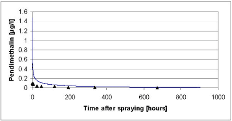
Figure 5.7 Simulated versus measured total concentration in the water column of pendimethalin for the artificial pond experiments of year 1999. The simulation was based on the data of Table 5.2 after modifications of the biodegradation and the diffusion in to the sediment discussed in the text.
Figur 5.7 Observeret og simuleret totalkoncentration af pedimethalin i vandsøjlen for det kunstige vandhulseksperiment i 1999. Simuleringen er baseret på data fra tabel 5.2 efter modifikation af bionedbrydningen og diffusion ind i sedimentet som diskuteret i teksten.
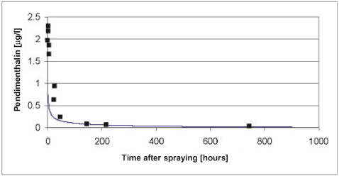
Figure 5.8 Simulated versus measured total concentration in the water column of pendimethalin for the artificial pond experiments of year 2000. The simulation was based on the data of Table 5.2 after modifications of the biodegradation and the diffusion in to the sediment discussed in the text.
Figur 5.8 Observeret og simuleret totalkoncentration af pendimethalin i vandsøjlen for det kunstige vandhulseksperiment i 2000. Simuleringen er baseret på data fra tabel 5.2 efter modifikation af bionedbrydningen og diffusion ind i sedimentet som diskuteret i teksten.
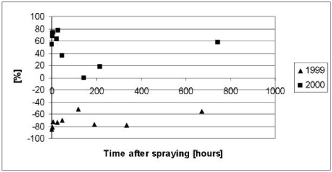
Figure 5.9 Residuals or relative difference between the simulated and measured total concentrations of pendimethalin in the water column of the experiments with artificial ponds in year 1999 and 2000. The simulation was based on the data of Table 5.2 after modifications of the biodegradation and the diffusion in to the sediment discussed in the text.
Figur 5.9 Residualer eller relative forskelle mellem den observerede og simulerede totalkoncentration af pendimethalin i vandsøjlen for det kunstige vandhulseksperiment i 1999 og 2000. Simuleringen er baseret på data fra Tabel 5.2 efter modifikation af bionedbrydningen og diffusion ind i sedimentet som diskuteret i teksten.
Table 5.4 Original K1 and K2 values of the procedure for extrapolation of biodegradation data to field condition proposed by Helweg et al., (2003) and the data suggested after calibration of the model for pendimetahlin against data from the experiments with artificial ponds.
Tabel 5.4 Originale K1 og K2-værdier fra poceduren for extrapolation af biodegraderingsdata til markforhold, foreslået af Helweg et al., (2000) og data foreslået efter kalibrering af modellen for pendimethalin mod data fra eksperimentet med kunstige vandhuller.
| K1 | K2 | |
| Original value of Helweg et al., (2003) | 1.85e-5 | 0.25 |
| Value after calibration | 1.85e-5 | 2e-3 |
5.3.2 Bentazon
According to Table 5.3 the disappearance of Bentazon from the water column is only dependent on the photolytic decay, which in turn is dependent on the macrophyte cover, shading from trees and structures around the ponds and on the attenuation of light in the water column. Following an examination of different combinations of shading and light attenuation in the water column a light attenuation coefficient of 2.5 (base 10) and a macrophyte cover of 50% was selected. We are aware of that the model systematically overestimates the Bentazon concentrations in the period from 72 to 1300 hours after the spraying. However it was not possible to avoid this, without causing a severe underestimation of the concentrations at the very end of the experimental period. A possible explanation of this limitation of the model might be that Bentazon not is distributed equally in the water column through the entire experiment but tend to concentrate in the upper layer immediately after the spraying due to a limited mixing of the water column (Helweg et al., 2003). Enhanced concentration of Bentazon in the upper layer of the water column is not taken in to account by the model, which assume that the water column is well mixed. This assumption might cause an overestimation of the light attenuation in the water column and consequently an underestimation of the photolytic decay of Bentazon.
Figure 5.10 Simulated versus measured total concentration in the water column of Bentazon for the artificial pond experiments of year 2000. The simulation was based on the data of Table 5.2 and the calibration of light attenuation and macrophyte cover discussed in the text.
Figur 5.10 Observeret og simuleret totalkoncentration af bentazon i vandsøjlen for det kunstige vandhulseksperiment i 2000. Simuleringen er baseret på data fra Tabel 5.2 og kalibreringen af lystilbageholdelse og makrofytdække diskuteret i teksten.
Figure 5.11 Residuals or relative difference between the simulated and measured total concentrations of Bentazon in the water column of the experiments with artificial ponds in year 1999 and 2000. The simulation was based on the data of Table 5.2 and the calibration of light attenuation and macrophyte cover discussed in the text.
Figur 5.11 Residualer eller relativ forskel mellem simuleret og målt totalkoncentration af bentazon i vandsøjlen i experimentet med kunstige vandhuller i 1999 og 2000. Simuleringen er baseret på data fra Tabel 5.2 og kalibreringen af lystilbageholdelse og makrofytdække diskuteret i teksten.
5.4 Verification of pesticide model for artificial ponds
As described in section 5.1.1 the pesticides of Glyphosate, Ioxynil and Fenpropimorph were selected for verification of the pond model. In addition, the pond experiment with pendimethalin, where the macrophytes were removed, was used for verification. The data used for verification appears from Table 5.5. As a part of the verification the uncertainty of the input parameters were taking in to account with the aid of a so called intelligent Monte Carlo analysis, which is described by Styczen et al., 2004b. On the basis of the intelligent Monte Carlo analysis was it possible to calculate 95% confidence intervals for the output of the model.
Table 5.5 Pesticide data used for the verification of the pond models. In addition, the data for ioxynil of Table 5.2 was used for verification.
Tabel 5.5 Pesticiddata brugt til verifikation af vandhulsmodellerne. Desuden blev data for ioxynil fra tabel 5.2. brugt til verifikation.
| Process | Pesticide | |||||
| Glyphosate | Pendimethalin | Fenpropimorph | ||||
| Value | Reference | Value | Reference | Value | Reference | |
| Desorption [h-1] particles | 0.46 | Calculated | 0.07 | Calculated | 0.25 | Calculated |
| Desorption [h-1] macrophytes | 0.048 | Calculated | ---- | Calculated | 0.069 | Calculated |
| Kd [m3g-1] | 7.6e-5 | EPA data base | 0.00051 | Helweg et al., 2003 Mangles 1990* |
0.00014 | Raedeker 1979* |
| Koc [m3g-1] | n.d. | ---- | ---- | Helweg et al., 2003 | 0.042 | Raedeker 1979* |
| Alk. Hydrolyse [h-1mol [H+] –1] | 0 | EPA data base | 0 | EPA data base | 0 | EPA data base |
| Acid Alk. Hydrolyse [h-1mol [OH-] –1] | 0 | EPA data base | 0 | EPA data base | 0 | EPA data base |
| Neutral Hydrolysis [h-1] | 0 | EPA data base | 0 | EPA data base | 0 | EPA data base |
| Pka | 2.74 | EPA data base | 2.8 | EPA data base | 7.0 | EPA data base |
| Bio_deg_water column [h-1] | 1.5e-4 | EPA data base | 0.015 | Helweg et al., 2003 | 4.2e-4 | Mühll 1990* |
| Bio_deg_pore_water [h-1] | 0.0055 | EPA data base | 0.39 | Helweg et al., 2003 | 0.015 | Mühll 1990* |
| Gas_exchange [mh-1] | 45 | Asman et al. 2003 | 45 | Asman et al. 2003 | 45 | Asman et al. 2003 |
| Liquid_exchange [mh-1] | 0.029 | Asman et al. 2003 | 0.029 | Asman et al. 2003 | 0.029 | Asman et al. 2003 |
| Water solubility (mg/l) | ---- | -------- | -------- | ----------- | 3.53 | Raedeker 1988* |
| Vapour pressure | ---- | ------ | -------- | ----------- | 1.7e-5 | Raedeker 1988* |
| Mol weight | ---- | ------ | ------- | ---------- | 303 | ------ |
| Henrys constant (-) | ---- | ----- | 1.10E-03 | EPA data base | 8.0e-5 | Calculated |
| Quantum Yield | ---- | ----- | ----- | ------- | -------- | ---------- |
| Photolysis rate [h-1] | ---- | ----- | 0.001 | Sanders, P. 1985 * | 0 | EPA data base |
| Retention in sediment | 28 | EPA data base | 256 | Calculated from Kd | 70 | Calculated |
In brief the intelligent Monte Carlo consisted of a selection of the most important process for each substance and a Latin Hyper Cube sample of the input parameters for the process assuming that each input parameter follows a log normal distribution. However, to take the uncertainty of the estimates of the mean and the standard deviation of each parameter caused by the low sample size in to account the normal distribution was substituted with a t-distribution. When the Latin Hyper Cube sampling was conducted it was assumed that the correlation's between the input variables was equal to 0. This assumption might be invalid for some pesticides. However, the data do not allow an estimation of the correlation since the input variables are estimated in separate experiments/systems and the correlation can therefore not be estimated. It was therefore decided to set the correlation to 0. The process selected for each compound appears from Table 5.6. The process was selected in accordance with the decision support trees of Styczen et al 2004.
Table 5.6 The most important process for the verification of the pond model for ioxynil, fenpropimorph, glyphosate and pendimethalin. The process was selected on the basis of the pesticides properties of Table 5.5 and the decision trees of chapter 8 in Styczen et al., (2004).
Tabel 5.6 De vigtigste processer for verifikationen af vandhulsmodellen for ioxynil, fenpropimorph, glyphosate and pendimethalin. Processerne er udvalgt på basis af pesticidegenskaberne i Tabel 5.6 og beslutningsstøttetræet i kapitel 8 i Styczen et al. (2004b).
| Active substance | Selected process |
| Pendimethalin | Effective diffusion in to sediment Degradation in sediment |
| Fenpropimorph | Effective diffusion in to sediment Degradation in sediment |
| Ioxynil | Effective diffusion in to sediment Photolytic degradation |
| Glyphosate | Effective diffusion in to sediment Degradation in sediment |
5.4.1 Glyphosate
The results of the verification for glyphosate appear from Figure 5.12. The model tends to underestimate the concentrations in the water column during the first hours after the spraying of glyphosate, whereas the model tend to overestimate the concentrations at the end of the experiment. An explanation could be that the process of diffusion and sorption into the sediment is overestimated, whereas the process of degradation in the sediment is underestimated. Diffusion could be overestimated because sorption of glyphosate is caused by ionic interactions, whereas the sorption of pendimethalin, for which the effective diffusion coefficient was calibrated, is due to hydrophobic interactions. Hence the effective diffusion coefficient might not be valid for glyphosate, which penetrates in to deeper parts of the sediment than Pendimethalin, which is trapped in the upper layer of the sediment rich in organic matter.
A straightforward explanation for the underestimated biological degradation cannot be given. However, it must be emphasised that the calibration of the biodegradation was done for pesticides with other sorption properties that glyphosate. This influences the results because the model takes sorption properties in to account when the bio-degradation is calculated.
Figure 5.12 Upper and lower limit for a 95% confidence interval for the simulation of glyphosate in the ponds with macrophytes in year 1999 plotted against the measured values.
Figur 5.12 Øvre og nedre grænse for et 95% sikkerhedsinterval for simuleringerne af glyphosat i vandhullerne i år 1999 plottet overfor de målte værdier.
5.4.2 Pendimethalin
The results of the verification for pendimethalin appear from Figure 5.13.
Figure 5.13 Upper and lower limit for a 95% confidence interval for the simulation of pendimethalin in the ponds without macrophytes in year 2000 plotted against the measured values.
Figur 5.13 Øvre og nedre grænse for et 95% sikkerhedsinterval for simuleringerne af pendimethalin i vandhuller uden makrofytter i år 2000, plottet overfor de målte værdier.
The model tends to underestimate the concentrations of pendimethalin. The deviations between the measured and simulated values are most pronounced in the beginning of the experiment. As discussed in section 5.2.4 the fate of pendimethalin is mainly driven by the diffusion and subsequent sorption in the sediment. Hence, the deviation can be explained by the choice of an average value for the effective diffusion coefficient.
5.4.3 Fenpropimorph
The results of the verification for fenpropimorph appear from Figure 5.14 to Figure 5.15. The model tend to overestimate the measured values in 1999, whereas the measured values tend to be underestimated in the year of 2000 irrespectively of the presence or absence of macrophytes. The deviations between the measured and simulated values are most pronounced in the beginning of the experiment. As for pendimethalin, the fate of fenpropimorph is mainly driven by the diffusion and subsequent sorption in the sediment. Hence, the deviation can be explained by the choice of an average values for the effective diffusion coefficient. However, generally the measured values lie within the 95% confidence intervals and the deviation caused by the choice of an average effective diffusion coefficient is generally balanced by the uncertainty on the input parameters.
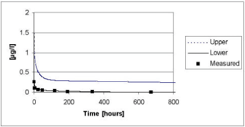
Figure 5.14 Upper and lower limit for a 95% confidence interval for the simulation of fenpropimorph in the ponds with macrophytes in year 1999 plotted against the measured values.
Figur 5.14 Øvre og nedre grænse for et 95% sikkerhedsinterval for simuleringerne af fenpropimorph i vandhullerne med makrofytter i år 1999 plottet overfor de målte værdier.
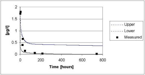
Figure 5.15 Upper and lower limit for a 95% confidence interval for the simulation of fenpropimorph in the ponds with macrophytes in year 2000 plotted against the measured values.
Figur 5.15 Øvre og nedre grænse for et 95% sikkerhedsinterval for simuleringerne af fenpropimorph i vandhullerne med makrofytter i år 2000 plottet overfor de målte værdier.
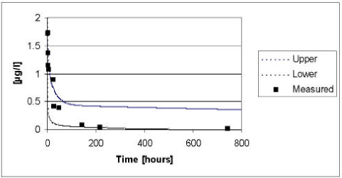
Figure 5.16 Upper and lower limit for a 95% confidence interval for the simulation of fenpropimorph in the ponds without macrophytes in year 1999 plotted against the measured values.
Figur 5.16 Øvre og nedre grænse for et 95% sikkerhedsinterval for simuleringerne af fenpropimorph i vandhullerne uden makrofytter i år 1999 plottet overfor de målte værdier
5.4.4 Ioxynil
The results of the verification for Ioxynil appear from Figure 5.17. The measured values fall almost right between the upper and lower limit of the 95% confidence interval.
5.5 Conclusion on the calibration and verification
The properties of the pesticides (Table 5.3) dictated that it only was relevant to consider the process of photolysis, biological degradation in the sediment and the diffusion and subsequent sorption in the sediment when the calibration was conducted. A calibration of the remaining process implemented in the model will require data for pesticides with other properties or a more detailed measurement programme. The verification revealed that the effective diffusion coefficient determined through the calibration exercise is not valid for glyphosate. In addition, the effective diffusion coefficient differ from year to year. This is not taken into account by the model but this effect is to certain extent balanced by the uncertainty of the input parameters.
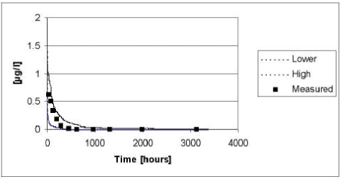
Figure 5.17 Upper and lower limit for a 95% confidence interval for the simulation of Ioxynil in the ponds with macrophytes in year 1999 plotted against the measured values.
Figur 5.17 Øvre og nedre grænse for et 95% sikkerhedsinterval for simuleringerne af ioxynil i vandhullerne med makrofytter i år 1999 plottet overfor de målte værdier.
6 Calibration and Validation of Pesticide Transport in the Catchment
- 6.1 Procedure
- 6.2 Simulation Results
- 6.3 Pesticide in drains
- 6.4 Uncertainty on the results caused by uncertainty on Koc and DT50
6.1 Procedure
A procedure for validation of pesticide simulations was outlined in the first status report of the project (DHI et al., 2000).
The proposed procedure includes the following steps:
- Calibration and validation of the water flow module.
- Blind simulation of the pesticide concentration in upper groundwater, and of concentrations and load in drain and stream. For drains, colloid-bound pesticide may be evaluated in some of the events.
- If pesticide data allows, calibrate pesticide load and concentrations in drain and upper groundwater on data from year 1 and validate on year 2. For drains, colloid-bound pesticide may be evaluated in some of the events.
- If the same pesticide is applied above more than one drain, calibrate pesticide parameters on one drain and validate on the second drain. For drains, colloid-bound pesticide may be evaluated in some of the events.
- Calibrate loads and pesticide concentrations in the drains and upper groundwater and validate on pesticide concentrations in the stream. This step is complicated by the fact that the stream may receive drainage water from point sources such as farmyards.
Some pesticides are not applied to areas near the monitored drains, and for these pesticides only the load and concentration in the stream can be evaluated.
The descriptions of colloid transport in the drain and the transformations of pesticide in the river were tested in more detail elsewhere.
The calibration exercises mentioned in step 2 and 3 require that the same pesticide be applied to an area two years in a row or to two different drains.
During the calibration it is necessary to start at the beginning of the season 1998, and work forward in time with the different pesticides. If earlier applications are known, the earliest may be considered the starting point. Pesticides with a widespread use have higher priority in the beginning of the calibration phase. Pesticides with limited area coverage may influence the general parameterisation in certain areas of the model. The aim of the processes is to gain a picture of how much the calibration is improved with more information about new pesticides and the spatial distribution of pesticides.
6.2 Simulation Results
The calibration procedure implemented included steps 1 and 2 mentioned in Section 6.1. Furthermore, drains were included in the evaluation for Lillebæk to the extent possible (step 3, 4). The pesticides bentazon, Terbutylazin, isoproturon and pendimethalin were selected for analysis. They were selected because they were detected in the stream of both Odder Bæk and Lillebæk.
It should be noted that due to the fact that some fields with pesticide applications exist in the field records without having a location on the field map, there is some uncertainty related to the actual applications of pesticide, particularly in Odder Bæk. In addition, pesticide application on farmyards and the like are not recorded in the data. Figures showing the locations of spraying and the loads of pesticide for each of the four pesticides for the three spraying seasons (1997-1998, 1998-1999, 1999-2000) for Odder Bæk and Lillebæk are shown in Appendix E and F, respectively.
The data used for the blind simulation mentioned in step 2 in Section entailed the application of the data on pesticide sorption and degradation from the Danish Environmental Protection Agency, given in Section and the data in Appendix D.
6.2.1 Odder Bæk
The results of the simulation of pesticide transport in Odder Bæk are shown in Figure 6.1, which shows the observed and simulated pesticide concentration in the stream at the outlet of the catchment and in the drain upstream (The location of the monitoring stations are shown in Figure 1.3). The simulation period was 1/7-1997 to ultimo 2000, but only the periods with detections and with simulated pesticide appearance in the stream and drain are shown.
Generally, pesticide concentrations in the right order of magnitude could be obtained with the blind calibration. Only in the case of isoproturon, further adjustment of the Kd and DT50 values were necessary. With the standard parameters, too little isoproturon leaching was simulated, and a two-fold reduction of the sorption (Koc decreased from 125 l/kg in the standard setup to 62.5 l/kg) and a two-fold increase in degradation (the half life time DT50 increased from 8 to 16 days) improved the match between observed and simulated concentrations. Overall, the organic matter content of the soil in the Odder Bæk catchment was decreased by a factor of two, in order to improve the simulation of all four pesticides. This was considered appropriate, as the measured values generally were very high. For the soil types that were categorised as organic, no data from measurements were available and hence the organic matter contents were estimated anyway.
The simulated pesticide concentrations were comparable to the observed levels. However, the dynamics, with distinct leaching peaks, concurrent with flow events, which is apparent from all pesticides, could not be captured satisfactorily by the model. This was most likely due to intermittently fast transport through macropores in the soil. Originally, Odder Bæk was selected to represent a sandy catchment without macropores, and thus one type of scenario. The decision not to include macropores goes back to the beginning of the project. However, this assumption was found not to hold true. The need for inclusion of macropores becomes even more evident in the case of pendimethalin where absolutely no leaching could be simulated with the standard parameters due to the exceptionally high sorption potential of this pesticide. The detection of Pendimethalin in the stream on several peak flow occasions is a clear indication of the presence of macropores, which enables a partial bypass of the upper soil layers that hold the largest sorption and degradation potential.
In the existing model description, the pesticides are leached to the stream through vertical matrix flow in the unsaturated zone and through fast or slow groundwater. This flow pattern, combined with the fact that no degradation in the saturated zone was assumed, entailed a subdued response, a too high background concentration, and an overall too high flux.
Another factor governing the response time of the leaching to the stream is whether drains are being activated. To obtain a fast response in the stream, drain flow, which bypasses lateral transport in the groundwater, is necessary. Drain flow is governed by the rise of the groundwater table to the drain depth and hence the intersection of these two in time and space becomes important. Especially, this could explain why only little leaching to the stream of Terbutylazin is taking place in the model. Terbutylazin is only applied on a small part of the catchment – in 2000, where the highest concentrations are found, it is only applied to two fields of which one is on the boarder of the catchment. In the model, the other field is drained but it does not contribute much with drain flow.
Another uncertainty related to the drained areas is the specification (location and extension) of the contributing area to the upstream drain where pesticide content has been monitored separately. In the case of Isoproturon, the simulated concentrations are too low, whereas in the case of Bentazon, the simulated concentrations are too high. A number of fields receiving isoproturon were situated just next to the area assumed to drain to the drain station. A slight shift in the defined drainage area will thus change the simulated concentrations. Furthermore, the drain is situated in an area of organic soil, for which no details concerning the soil description is available. The content of organic matter in this soil is thus guessed.
Finally, the observations can be influenced by point sources, e.g. a spill more or less directly into the water body. The peak on June 12, 1999 in bentazon concentration downstream does not occur in direct association with known applications inside the catchment. The last pesticide application immediately before the peak event was on May 28 and two samples after this date (on June 6 and 9) did not contain the pesticide, indicating that field application most likely was NOT the source.
In conclusion, the response in Odder Bæk is simulated with the right level of concentrations, but it is somewhat subdued, with a high background concentration presumably due to the model assumptions of no macropores and no degradation in the saturated zone. Furthermore, model uncertainties are related to the drain specifications. Finally, Some detections could be influenced by point sources and hence not regular surface applications as assumed in the model.
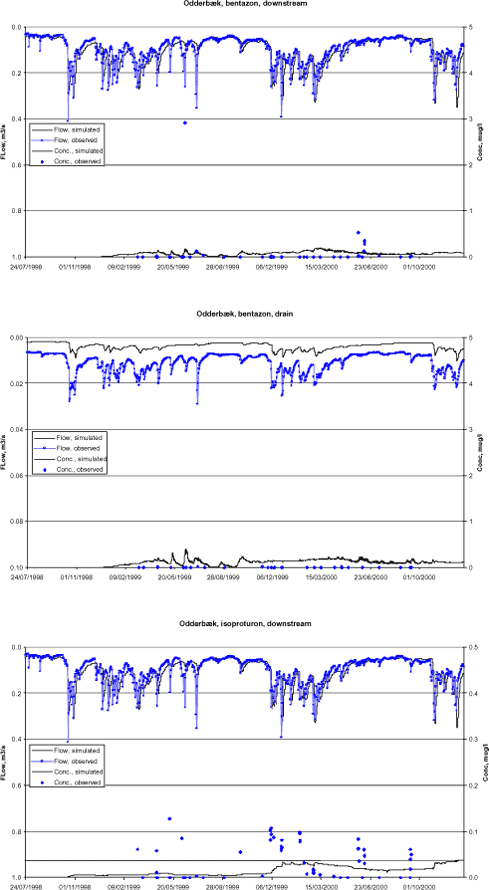
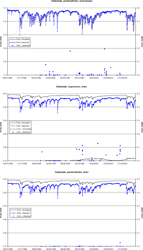
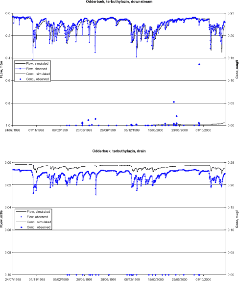
Figure 6.1 Simulated and observed flow and pesticide concentration in Odder bæk.
Figur 6.1 Simuleret og observeret afstrømning og pesticidkoncentration i Odder bæk.
6.2.2 Lillebæk
The results of the simulation of pesticide transport in Lillebæk are shown in figure 6.2. The figure shows the pesticide concentration at the downstream and upstream measuring station. The simulation period was 1/1-1997 to ultimo 2000, but only the period 1/7-1997 to ultimo 2000 are shown, because no observed nor simulated pesticide occurred in the stream during the first half year of the simulation period.
6.2.2.1 Bentazon
For bentazon, less leaching is simulated in the upstream than the downstream station, which is in accordance with the pesticide application source locations. Except for the two occurrences in the spring of 1999 upstream and the occurrence in the fall of 1999 downstream, the levels simulated are in good agreement with the observations. The peak observed upstream in 1999 is most likely a point source, as only a very small field (0.4 ha), received bentazon in the spring of 1999, prior to the peak.
The peak observed downstream in the fall of 1999, however, can be explained by antecedent field applications. The reason for not simulating the peak could be that the drains on the fields receiving bentazon were not activated in the model during this period. One and a half months later, the simulated concentration increased, which probably reflects a delay of the breakthrough observed. The concentration simulated is then lower than observed in the peak. In the model, drain water stem from the upmost groundwater layer. This means that infiltrating water becomes mixed with water that percolated at an earlier stage, causing dilution. The limitation to the depth of the upmost calculation layer is that it has to include the full groundwater fluctuation. In reality the infiltrating water may not be mixed in such a large volume of water giving rise to higher concentrations.
Bentazon is applied exclusively in the spring, and according to the model, is primarily leached in the late fall, winter and spring periods. Downstream, more continuous leaching is simulated in the summer of 2000. This could be explained by the fact that no degradation is occurring in the model, below 1 m in the unsaturated zone, and in the saturated zone. Hence, pesticide that has entered the saturated zone, and is not captured by the drains, will eventually reach the stream in unaffected concentrations, whereas in reality, some degradation may occur in the shallow groundwater.
6.2.2.2 Isoproturon
Looking at the results for isoproturon, more leaching is simulated upstream than downstream. This is accordance with the location of sources, as more fields are located upstream of the upstream station than downstream. Also, the degradation potential is relatively high for isoproturon yielding a degradation also during the transport from the upstream to the downstream station.
There is a distinct pattern of heavy leaching in the spring and summer of 1998 and 2000, with less leaching in 1999, which reflects the intensive use of isoproturon in the fall of 1997 and 1999. Leaching persists through the summer months though applied in the fall the anterior year, and despite the fact that the sorption and degradation potential for isoproturon is higher than for bentazon. This could explained by the fact that the fields receiving isoproturon are located relatively far from the stream and that some degradation actually occurs in the groundwater, as opposed to the model description.
The downstream peak, observed on Oct. 23-24, is most likely not a point source as fields close to the downstream station are sprayed closely before. The reason for not capturing the peak in the model is, as the case was for bentazon, that the drains have not been significantly activated at this time.
To test whether the exagerated simulated isoproturon concentrations during 1999 and late 2000 could, as hypothesized above, be explained by a lack of degradation in the lower part of the soil profile and in the groundwater, an additional simulation was performed, in which degradation in the unsaturated zone (below 1 m) as well as in the groundwater was set to the same as defined for the soil layers between 0.8 and 1.0 m depth. The results are shown in Figure 6.3.
It is seen that the simulation is significantly improved, as the tailings from the previous pesticide application is deminished due to the additional degradation in the lower layers. This effect will be greatest for the pesticides with the highest degradation portential, and pesticides with sources furthest away form the stream. Of the four pesticides, isoproturon has the highest degradation potential, and hence the effect will be relatively larger here. However, when comparing the simulation results for isoproturon with the other three pesticides, this is also the one, that has the largest problem with exagerated talings. This could indicate that either too much is transported to the groundwater or that degradation does take place to some degree in the upper groundwater.
6.2.2.3 Pendimethalin
Leaching of pendimethalin, as opposed to in the Odder Bæk catchment, could be simulated in Lillebæk. This is because macropore flow and transport is included in the setup of Lillebæk.
The pattern of leaching of pendimethalin is comparable to the leaching pattern of isoproturon, which is because the fields and application times are very comparable. However, more downstream than upstream leaching is, simulated, as opposed to bentazon, because relatively more fields downsream of the upper station are receiving pendimethalin, but not isoproturon.
A better correspondence with observations is obtained for pendimethalin during the second half of 2000 than for isoproturon, due to lower degradation rates and hence less influence of the transport, and potential degradation, in groundwater.
Again, a discrepancy is observed between observations and simulations in the the beginning of the drainage season, in this case, both upstram and downstream. Point sources are not suspected, as peaks succeed all applications registered in the fall of 1999. Again, the lack of initial drain flow could explain thia discrepancy.
6.2.2.4 Terbuthylazin
The response pattern of terbuthylazin is very similar to that of bentazon. This is because terbuthylazin is also applied in the spring, and the number of fields sprayed, and in some cases, the location of fields, are the same. The concentration levels are, however, larger for terbuthylazin than for bentazon. Looking at the sorption and degradation potantial for the two pesticides, terbuthylazin is more persistent and more sorptive, which may partly outbalance each other. However, the unit doses applied in the case of terbuthylazin are significantly higher than for bentazon (56, 89, 13 % higher in the seasons 1997-1998, 1998-1999, 1999-2000), which may partly explain the higher concentrations.
When comparing the model results with the observations, it is obvious that much higher concentrations have been detected in the stream (especially upstream) than have been simulated. This is most likely due to unknown point sources that are not accounted for in the model. Upstream, the maximum concentrations are: 4.318 μg/l (obs., not shown) vs. 0.103 μg/l (sim.), whereas downstram, the maximum concentrations are: 0.330 μg/l (obs.) vs. 0.088 μg/l (sim.). This issue is discussed further in section 7.2. The observed concentrations are generally much higher upstream than downstream.
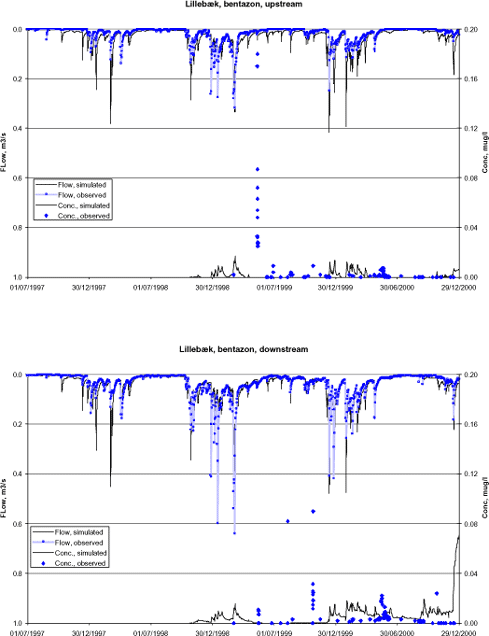
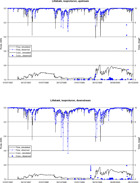
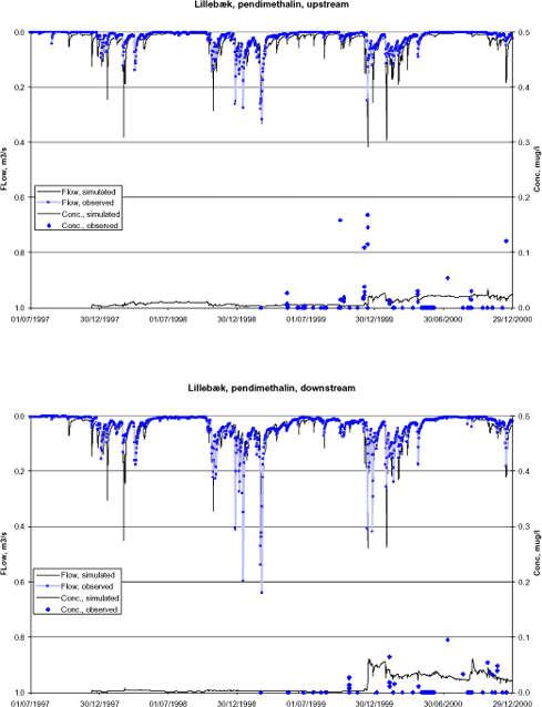
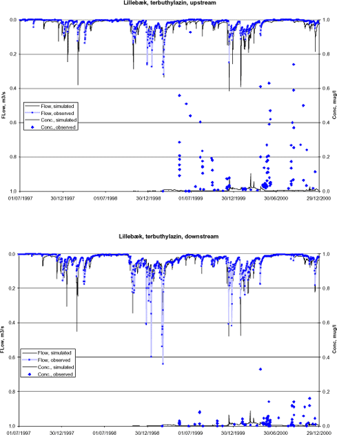
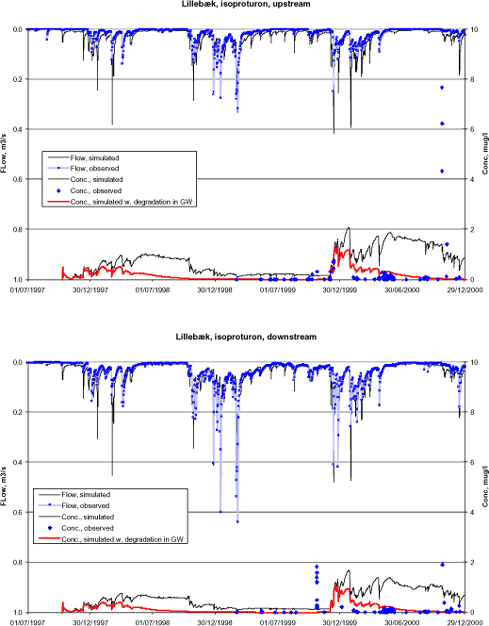
Figure 6.2 Simulated and observed flow and pesticide concentration in Lillebæk.
Figur 6.2 Simuleret og observeret afstrømning og pesticidkoncentration i Lillebæk.
Figure 6.3 Simulated and observed flow and isoproturon concentration in Lillebæk. An additional simulation with degradation in lower layers and in groundwater has been included.
Figur 6.3 Simuleret og observeret afstrømning og isoproturonconcentration i Lillebæk. En ekstra simulering med nedbrydning i dybere lag og i grundvandet er inkluderet.
6.3 Pesticide in drains
Table 6.1 shows the pesticides sprayed in the two monitored drain areas in Lillebæk. The compounds, which are not monitored, are indicated in gray in the table. It is obvious that the chance of modelling pesticides on a drain is much better for drain 6 than for drain 2. However, only a few compounds are used on the same field two years in a row or on both drain 2 and drain 6.
Table 6.1 Pesticides applied on the catchment areas of drain 2 and 6 in Lillebæk. "Gray" pesticides are not monitored.
Tabel 6.1 Pesticid udbragt på markerne til dræn 2 og 6 i Lillebæk. "Grå" pesticider har ikke været moniteret.
| Drain | 6 | 2 | ||
| Field | 404 | 403 | 404.1 | 1803 |
| Year | ||||
| 1998 | Desmedipham Esfenvalerat Ethofumesat Metamitron Phenmedipham Pirimicarb |
Bromoxynil Ioxynil Fenpropimorph Propiconazol |
Bromoxynil Ioxynil Isoproturon Fluroxypyr Fenpropimorph Propiconazol Azoxystrobin |
Esfenvalerat Haloxyfob-ethoxyat |
| 1999 | Bentazon Fenpropimorph Pendimethalin Propiconazol |
Esfenvalerat Fenpropimorph MCPA-mixture Propiconazol |
Azoxystrobin Fluroxypyr Glyphosat Metsulfuron-methyl Pirimicarb Tebuconazole |
Bromoxynil Chlopyralid Fenpropimorph Floroxypyr Ioxynil Propiconazol |
| 2000 | - | Chlopyralid MCPA Mechlorprop |
Bentazon Pirimicarb |
Diflufenican Esfenvalerat Isoproturon Tebuconazole |
Table 6.2 Detection of sprayed pesticides on drain 6 in the Lillebæk catchment.
Tabel 6.2 Fund af udbragte pesticider på dræn 6 i Lillebæk-oplandet.
| Dræn 6 | Positive obs. | Conc, ng/l | 1999 | 2000 |
| Bromoxynil | 1 | 1 | 17/2 | |
| Ioxynil | 0 | |||
| Ethofumesat | 0 | |||
| Fenpropimorph | ||||
| Bentazon | 5+11 | 1; 76; 3; 3; 3 3;3;2;2;1;1;3; 2;2;2;1 |
3/3,20/8, 9/10,9/10, 10/10 |
17/2, 17/2, 18/2, 18/2, 21/2, 27/3, 10/4, 24/4, 25/4, 25/4, 25/4; |
| Isoproturon | 4+8 | 61; 5; 1; 1; 90; 79; 49; 3;3; 66; 30; 171 |
3/3, 9/10, 9/10, 10/10 |
17/2, 18/2, 18/2, 27/3, 24/4, 25/4, 25/4, 4/12; |
| Metamitron | 0 | |||
| Propiconazol | 1 | 2 | 20/8 | |
| Pirimicarb | 0 | |||
| Phenmedipham | 0 | |||
| Pendimethalin | 3 | 7; 4; 26 | 9/10, 9/10, 12/12 | |
| MCPA | 0 | |||
| Mechlorprop | 1 | 3 | 9/10 | |
| Metsulfuron-methyl | 0 |
First spraying of Bentazon on drain 6 is 6/5, 1999, the second is 30/4, 2000. The measurement on 3/3, 1999 thus cannot be explained by the sprayings in 1999 or 2000.
Isoproturon has only been used on the area in 1998, on 20/10, 1997. The detection in December 2000 cannot be explained by any registered sprayings on the drain.
Propiconazol is sprayed on 15/6, 1998, and 14.6, 1999, but is only found in the autumn of 1999. Pendimethalin is sprayed on 6/5, 1999 and is found in the following autumn.
Mechlorprop is applied on 29/4, 2000, and the detection on 9/10, 1999 therefore cannot be explained by the registered application.
It is worth noting that in spite of the fact that the area has macropores, the detections are not necessarily closely tied to the time of application.
Table 6.3 Detections of sprayed pesticide on drain 2 in Lillebæk catchment.
Tabel 6.3 Fund af udbragte pesticider på dræn 2 i Lillebæk-oplandet.
| Dræn 2 | Fund | Conc, ng/l | 1999 | 2000 |
| Bromoxynil | 1 | 1 | 23/4 | |
| Ioxynil | 1+1 | 1; 3 | 20/8 | 23/4 |
| Fenpropimorph | 0 | |||
| Isoproturon | 4+14 | 3; 5; 2; 5 74; 63; 1; 107; 78; 122; 4; 6; 3; 3; 3; 23000;1300;180 |
20/8, 24/8, 10/10, 15/11 |
2/2, 9/2, 17/2, 18/2, 18/2, 18/2, 3/3, 23/4, 8/5, 22/5, 6/6, 7/11, 20/11, 15/12 |
| Propiconazol | 4 | 4; 1; 1; 1 | 20/8, 24/8, 10/10, 15/11 |
Bromoxynil is applied on drain 2 on 7/9, 1999 and Ioxynil on 7/9, 1998 and 11/5, 1999. Fenpropimorph and Propiconazol are both applied 11/5, 1999. Isoproturon is applied on the drain on 6/10, 2000. The fact that it is found so often on the field before this date must be due to water entering the drain system from somewhere outside the field.
It is worth noting that a number of compounds are found in the drains in significant concentrations, but they are not recorded as applied in the monitoring period. Both Atrazin and two of its metabolites are found in drain 6 and must be a result of the fact that the field has been used for maize earlier. Hydroxyatrazin is found in 1999 in concentrations up to 224 ng/l. Terbutylazin and its metabolites are also found both years.
In drain 2, Hydroxy-carbofuran is found in concentrations of 1.6 μg/l on 30/9, 1999 and 1.1 μg/l on 1/10, 1999 without a known source. P-nitrophenol is found in both drains in concentrations up to 0.125 μg/l, again without a local source.
6.3.1 Pesticide simulations in drain areas in Lillebæk
Based on the analysis of pesticide applications and detections on drain 2 and drain 6 in Lillebæk in Section 6.3, only two combinations of pesticide and drain were found relevant:
bentazon on drain 6 and isoproturon on drain 2. Some data on the two are given in Table 6.4.
Table 6.4 Data on pesticide simulations in two drained areas in the Lillebæk catchment
Tabel 6.4 Data vedr. pesticidsimuleringer i to drænoplande I Lillebæk-oplandet.
| Drain2 | Drain6 | |
| Pesticide simulated | Isoproturon | Bentazon |
| Area | 4 ha | 2.5 ha |
| Number of grids simulated | 16 | 10 |
| Fields treated | 1803.0 on 6/10-2000 | 404.0 on 6/5-1999 404.1 on 30/4-2000 |
The results of the simulations are shown in Figure 6.4. It is seen that the drain flow is very well simulated. It should be remembered here that the drain flow results have been extracted from the hydraulic model without further fine-tuning to the smaller areas. The fine correspondence between observed and simulated flows on such a small scale gives credibility to the overall water balance simulations.
With respect to the pesticide transport, the isoproturon on drain 2 is very well simulated (Note that two plots are shown for isoproturon that have different scales on the pesticide concentration axis to the right). During most of the simulation period, the concentration is low. The peakiness of the occurrences are well described, and it should be noted that the distribution of rain intensities stem from a rainfall station away from Lillebæk. Total correspondence cannot be expected. Very high concentrations are measured and simulated at the end of 2000 (23 μg/l (obs.), 12.8 μg/l (sim)). In this case, it appears that the timing of the drain activation is correct, which was found to be a general problem for simulations of transport to the stream.
Bentazon leaching on drain 6 is somewhat over-simulated. A reason for this could that the soil types on drain 6 is not representative of the real soil types. Since the soil types, except for the lower part of the catchment, have been distributed randomly over calculation cells of the catchment, an error can be associated with the distribution of the soil types. On this particular soil sand occurs in the bottom of the column, and any macropore flow would end here and not be transported to groundwater. The exaggerated macropores caused by the present description of colloid transport may thus also influence the result.
Figure 6.4 Simulated and observed flow and isoproturon concentration in drain area 2 and bentazon concentration in drain area 6 in the Lillebæk catchment. Note the scale difference on the first two parts of the figure.
Figur 6.4 Simuleret og observeret afstrømning og isoproturonkoncentration i drænopland 2 og bentazonkoncentration i drænopland 6 i Lillebæk. Bemærk skalaforskellen på de første to delfigurer.
6.4 Uncertainty on the results caused by uncertainty on Koc and DT50
In order to evaluate the uncertainty caused by parameter values, it was decided to create runs that would represent the 95% boundary of leaching from the root zone. It is assumed that Koc and DT50 are independent within the range of the available data sets. In some cases, the data sets have been changed compared to the runs presented in . Data from the PATE-database have been supplemented with data from Lindhardt et al. (1997), and if more estimates of DT50 were made on the same soil, these were averaged before the information was used.
First, it was assumed that Koc and DT50 follow a log-normal distribution. The measured values were used to fit the ln(mean) and the corresponding standard deviation. For Koc for Bentazon and Isoproturon, values were available from Lindhardt et al. (1997) and the values were estimated both on the basis of the values from the PATE database alone and with the extra values. For the DT50-value for Isoproturon, the values in the database are based on two soils only, and the data from Lindhardt et al. (1997) contained information from one additional soil. The derived information is shown in Table 6.6.
Secondly, the mean and the standard deviation were used to create the distribution and it was assumed that the log transformed data are normally distributed. However, due to the fact that the number of observations is low, a t-distribution is used rather than a normal-distribution. This takes into account that the estimates of the standard deviation and the mean is associated with error due to a limited number of observations.
To create approximately a 95%-fractile, Koc and DT 50 values representing a 22.5 and 77.5 percentile are extracted. It is obvious that most leaching will occur when DT50 is high and Koc is low. Assuming that the two values are independent, two extremes combined will produce approximately a 95% fractile (0.2252 = 0.05).
The selected worst case/best case parameter combinations are shown in Table 6.5.
Table 6.5 Worst case/best case combinations of Koc and DT50 for the four pesticides simulated in the two catchments.
Tabel 6.5 Værste og bedste kombination af Koc og DT50 for de fire pesticider simuleret i de to oplande.
| Compound | Worst case | Best case | ||
| Koc | DT50 | Koc | DT50 | |
| Bentazon | 8.67 | 34.6 | 26.0 | 15.3 |
| Isoproturon | 72.8 | 12.1 | 159 | 7.26 |
| Terbutylazin | 191 | 106 | 303 | 54.8 |
| Pendimethalin | 13767 | 72.85 | 17431 | 59.55 |
Table 6.6 Mean, standard deviation and fractile values derived for four pesticides. If values were available from the PATE-database and from other sources (in the case of Bentazon and isoproturon), values have been calculated both for the PATE-values alone and for the combined dataset.
Tabel 6.6 Gennemsnit, standardafvigelse og fraktilværdier udledt for de fire pesticider. Hvis værdier fandtes i PATE-databasen og fra andre kilder (i tilfældet bentazon og isoproturon, er værdierne beregnet både for PATE-værdierne alene og for det kombinerede datasæt.
The results of the simulated best and worst cases are shown in Figure 6.5 and Figure 6.6 for Odder Bæk and Lillebæk, respectively. In the case of isoproturon in Odder Bæk. both stream and main drain yield concentrations and a total load, which are smaller than observed. Hence, the Koc and DT50 values had to be fine-tuned as described in to obtain results that were even more extreme than the worst case-scenario. In the case of Pendimethalin in Odder Bæk. even the worst case scenario did not generate leaching to the stream and hence no results are shown.
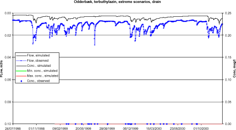
Figure 6.5 Simulated best and worst scenarios for the Odder bæk catchment for bentazon. isoproturon. and Terbutylazin. Observed concentrations in the stream and main drain are also shown.
Figur 6.5 Simulerede bedste og værste scenarier for Odder bæk-oplandet for bentazon. isoproturon. og Terbutylazin. Observerede koncentrationer i vandløbet og hoveddrænet er også vist.
For Bentazon in Lillebæk, the variation in parameters reduces the observed problems at the end of the simulation, but it does not remove it. The same is the case for isoproturon, which is still poorly simulated and seriously overestimated. Degradation in the groundwater zone is still required to improve the simulation. The variations given for pendimethalin hardly change the simulation. For Terbutylazin, the simulation is influenced during the winter 1999/2000 and the levels and peakiness of the simulation does change somewhat from the worst to the best case.
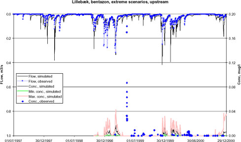
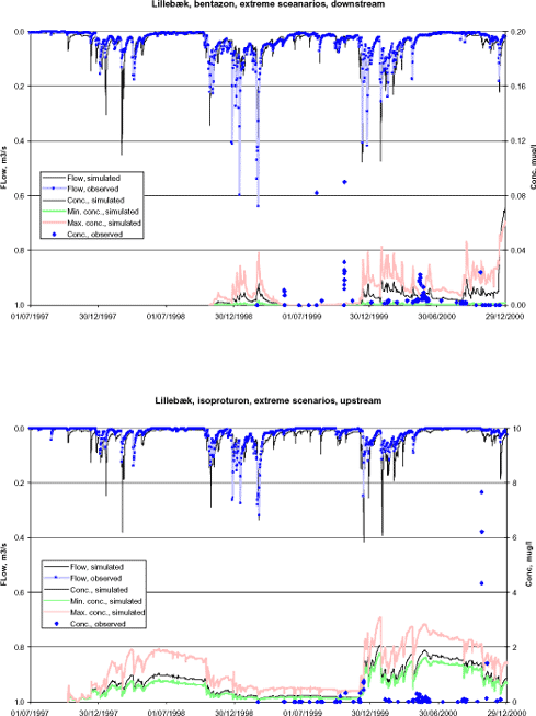
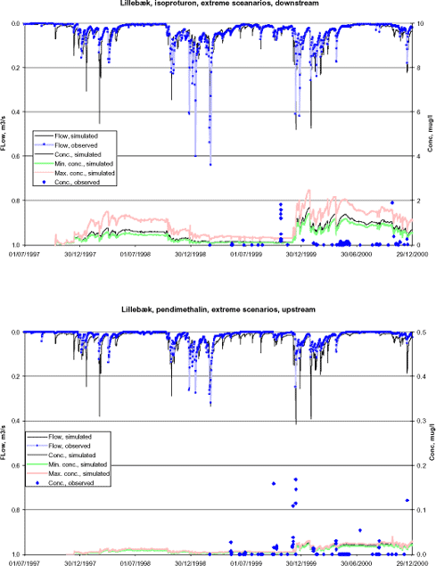
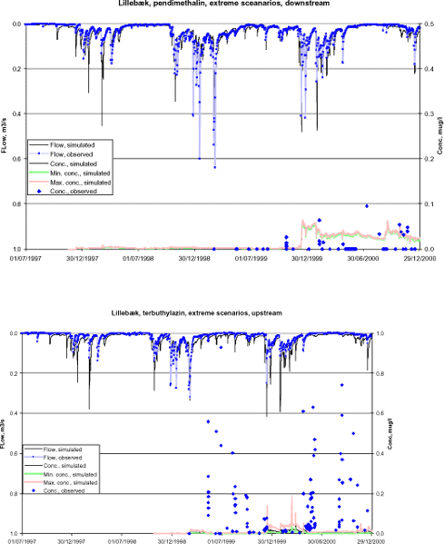
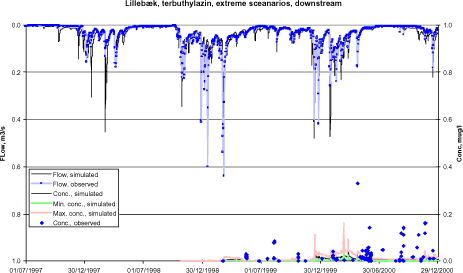
Figure 6.6 Simulated best and worst scenarios for the Lillebæk catchment for bentazon. isoproturon. pendimethalin and Terbutylazin. Observed concentrations downstream and upstream are also shown.
Figur 6.6 Simulerede bedste og værste scenarier for Odder bæk oplandet for bentazon. isoproturon. pendimethalin og Terbutylazin. Observerede koncentrationer nedstrøms og opstrøms er også vist.
7 Discussion
7.1 Choice of model
The overall approach chosen has been to model catchments rather than single fields. This approach has resulted in a very thorough quality control of existing data from the catchments. This check had not been possible if only a part of the hydrological processes had been simulated. It is a point in favour of the model that it does not allow inconsistencies in input and measured data.
An important point for generation of water to the stream is the dynamics of the groundwater level. In case the project had chosen to limit the model to root zone models only it would have been difficult to generate the correct groundwater levels required as lower boundary condition for each of the soil columns used in the simulation.
The transport of "old" pesticides during low-flow due to transport with groundwater is actually captured by the model and could not have been with a de-coupled approach.
The limitation of the overall approach is the runtime of the models. Simulations take a long time and this has limited the amount of tests possible and the storage space required for intermediate files have limited the precision to less than that was the original goal.
7.2 Process descriptions
It is obvious, however, from the simulations that some process descriptions require more attention.
It is a critical issue that the colloid description implemented does not describe the experimental data collected by sub-project 4. The process description seriously underestimates the transport of strongly sorbing compounds. In order to be able to believe the model results for this group of compounds, a better validated process description will have to be implemented.
The model shows a tendency of build-up of the applied compound in the upper layer of the saturated zone. At the same time it often undervalues the peak concentrations of pesticides. Pesticide may thus arrive in the stream in concentration peaks that are too low but occur too long.
This has to do with the basic structure of the MIKE SHE-model. The unsaturated zone is divided into small calculation layers but the upper layer of the saturated zone has to be able to absorb the variation in the groundwater level over the year. This variation may be several meters (at least 2 m in Odder Bæk and 5 m in Lillebæk. see Figure 4.5. Figure 4.6. Figure 4.7. Figure 4.8 and Figure 4.11). Drain flow is generated from the saturated zone when the groundwater rises above drain level. The following example may describe the effect: A saturated layer of 2 m with 0.3 as porosity contains 600 mm water under drain level. 20 mm of water percolates to the saturated zone with a concentration of 20 μg/l. When this water is mixed with the water in the calculation layer, the concentration is reduced to 0.645 μg/l. Only 3.2% of this water then leave immediately in the drain. The rest of the water will move towards the stream or the catchment boundary over time. The concentration in the groundwater will therefore tend to build up.
Particularly in Lillebæk where the groundwater variations are large, this is considered a serious problem. However, it is also observed on the Lillebæk soils that the drains are placed in a rather impermeable layer, meaning that water will tend to saturate layers in the soil above the true groundwater level. Presently, MIKE SHE does not allow this water to move to the drains, as drains are not implemented in the unsaturated zone. It is expected that the modelled peaks would improve if drains would be implemented in the unsaturated zone. This is so because the mixing to a large extend would be avoided and because the transport time to the drain would be reduced. A secondary effect of this would be that the solute that leaves the soil column about the groundwater does not contribute to build-up of pesticide in the saturated zone later on.
It was already from the beginning of the project decided to compare a clayey catchment with a sandy catchment. The changes that have taken place during the project concerning the interpretation of the Odder Bæk catchment have violated some of the initial assumptions. The most serious assumption from a calibration point of view is that macropores were not included (by definition). However, there are indications of presence of macropores in Odder Bæk. substantiated by the fact that subproject 4 measured colloid transport in the soils. It is likely that the process is more relevant on the JB3-4- topsoils than on the JB1-2-topsoils, but it may also occur where a sandy topsoil lies on top of a more clayey subsoil.
As discussed for Lillebæk some of the observed pesticide peaks may not be caused by ordinary field applications. For the monitored drains, the connection between application and detection is never instantaneous – usually spring applications are found in the following autumn. The very fast responses observed during the spraying season may thus, at least in some cases, reach the stream through other pathways. Indications of point sources are found in other studies.
In the county of Bornholm, 10 agricultural enterprises were investigated. Water samples were taken in secondary groundwater close to the soil surface. Samples were taken in the area of the farm itself and not on the fields. Pesticide concentrations measured were between 3 and 1720 μg/l for pesticides in total. For single compounds the concentrations were lower (maximum 800 μg/l). The large concentrations assumed to be caused by a considerable use of pesticides, inappropriate washing places for spraying equipment or inappropriate handling of pesticides (Bay. 2001).
For enterprises spraying for farmers (maskinstationer. 42 investigations on 40 sites) the picture is similar (Amternes Videncenter 2002). Pesticides were detected on 94% of the sites investigated. It is thought that there are more point sources with large concentrations than the study indicated.
J. Kreuger (1998) finds that Atrazin. Hexazinon, Propyzamid, Simazin og Terbutylazin (and to some extent Bentazon og Cyanazin) stems from applications on non-agricultural land such as farmyards. In a single case a farmyard resulted in a concentration in the stream of 100 μg/l. In total more than 6 kg of Terbutylazin was washed out over 7 months. Large concentrations of a number of pesticides were collected in water from farmyards. The leaching continued over several months. Furthermore, two cases of spill in connection with filling or cleaning of equipment were identified. In the conclusion of the paper is written: Indeed. a substantial contribution of pesticide loss to stream water was from the application of pesticides in farmyards.
German results (Müller et al., 2000) have shown that a very large part of the pesticide application (>77%) arrived to the stream through the sewer as farm runoff was connected to the sewer system. In the final empirical model developed, only the applied amount of pesticide is a significant variable equal to 43 g a.i. for each field sprayer in the catchment. Measured concentrations were between 0 and 23.18 μg/l.
In the present study, one observation of bentazon in Odder Bæk could be a point source (2.9 μg/l). It is not related to a particular spraying and the level is considerably different from the rest of the measurements. For Lillebæk, the high occurrence of Terbutylazin in May 1999 is judged to be a point source. It is not possible to model the fast breakthrough observed in spite of the exaggerated macropores. Considering that only two small areas are sprayed upstream of the measuring station the thinning factor is likely to be substantial and the concentration just under the root zone should be in the order of mg/l. A high concentration of Diuron was measured simultaneously, - Diuron was sprayed on one of the two fields (and in a smaller dose). The concentration below the root zone should therefore be even higher to create the observed concentration at the measuring station. Furthermore, Simazin was observed in a high concentration without any recorded use of the pesticide.
On this basis it seems unrealistic to expect that no point sources are present in the material from the two catchments. The question is whether the model has been calibrated unrealistically to catch events, which are point sources rather than field applications.
7.2.1 Parameter choice
With respect to parameter choice for the compounds, very few modifications were done. Basically the values deducted for the compounds came from the PATE database and were estimated as recommended in FOCUS (2000). The only modification that was made was that the organic content in the Odder Bæk soils were halved compared to measurements. This sounds as a drastic change, and is so with certain limitations. First of all the area around Odder Bæk is organic soil, and there were no local measurements of its actual properties, the depth of the organic layer etc. The values here were therefore rather arbitrary from the beginning but they greatly influence the simulated pesticide transport. The simulation of isoproturon on the area of drain 51 is underestimating the actual load. It is however not very clear whether this is due to the organic content or because the estimated drain area for drain 51 is erroneous. Just around the delineated drain area are several fields, which receive the same pesticide.
The organic content of the soils from the soil profiles of Odder Bæk shows 4-5% organic matter. This is considered to be a very high content, particularly on a sandy soil used for arable farming. In connection with nitrate simulations, it has been discussed whether the high content is due to a lower reactivity of the organic matter. On the other hand, the change in organic content could also be a compensation for the fact that macropores were not included in the model.
7.3 Steering parameters
With respect to discretisation in space, the main issue is the size of the upper saturated zone-layer already discussed above. Of course the horizontal discretisation of 50m also introduces errors but nothing in the simulations has raised concern about the effect of the presently used grid size.
For Odder Bæk the discretisation in time was thought not to be critical because macropores are not included. All pesticide has to enter the drains through the unsaturated zone, and this process is relatively slow compared to the calculation timesteps used.
Discretisation in time is critical for macropore simulations. For this reason the water simulation file for pesticide simulations in Lillebæk was generated with a rainfall file that was "faked": it contained the same monthly rainfall as measured by the local station but it was divided into intensities (6 min) according to measurements on a different station. This method allowed generation of colloids and transport in macropores in a very detailed manner. However, due to the limitation with respect to storage, the information is averaged over the storage time step (16 hours for the unsaturated zone in Lillebæk). The mass is thus conserved but the peaks become too flat.
This is difficult to counteract as it requires a more detailed storage of information in the intermediate files. Presently, it has not been possible to break the 4.2 gigabyte limit of one file. There are solutions to this problem but it requires e.g. that the MIKE SHE code is changed so that it switches to a new file when the limit is approached.
8 Evaluation of the Appropriateness of the Chosen Model for Description of Fate and Transport of Pesticides in Lillebæk and Odder Bæk Catchment
It is believed that the approach chosen is sound and that the combined simulation of all the involved processes is the most correct way to handle the pesticide movements at catchment scale.
It is however clear that some process descriptions and part of the parameterisation require further work. The two processes of particular concern are the colloid transport in the macropores and drain from the unsaturated zone. Presently it must be expected that the transport of strongly sorbing pesticides is distorted in the model and that peaks are lower than what may be the case in reality.
On the other hand, the simulation of Isoproturon on drain 2 in Lillebæk shows that the model description in some cases catches the observations surprisingly well and even over decades in concentration levels.
It must be concluded that the description of colloid transport and the parameterisation provided by Holm et al. (2003) is not adequate for use at catchment scale. The generated colloids moved around along the surface in huge amounts in the model and the parameterisation used at the end produced considerably less colloids. On the other hand, the colloid module requires the macropore description to be parameterised in a manner where exchange with the matrix is underestimated. All in all, macropore transport is considered being overestimated. It is thought that a better correspondence between observation and simulations could be obtained without the colloid description applied, and using a parameterisation of the macropores based on the profile descriptions.
On the other hand, macropores obviously should be included in the Odder Bæk description. However, then the area does not live up to the requirements specified in the beginning of the project, where the area was supposed to represent a very sandy site. With respect to Odder Bæk. the Danish Environmental Protection Agency has to consider whether it can be considered a reasonable catchment of registration purposes or whether a sandier site is required.
The third problem mentioned in the report is the discretisation at the border between the saturated and unsaturated zone, leading to thinning of peaks and probably too much transport to the groundwater. Furthermore, it is thought that the possibility of draining intermittent groundwater would improve the present description.
The model is not considered sufficiently well calibrated to be fully reliable. The levels of pesticide observed in the stream were in several cases reasonable, particularly at the top end of Lillebæk. However, the loads of pesticide moved through groundwater appear too large. The peakiness of the observations is much better described in Lillebæk than in Odder Bæk, due to the macropores, but this is to some extent overshadowed by the overestimated groundwater transport.
9 References
Allerup. Peter. Henning Madsen og Flemming Vejen (1998): Standardværdier (1961-90) af nedbørskorrektioner. Technical Report 98-10. DMI. 18 pp.
Amternes Videncenter (2002): Erfaringsopsamling – Amternes undersøgelser af pesticidpunktkilder. Teknik og Administration Nr. 2 2000. 78 pp.
Aslyng. H.C. and Hansen. S. (1982): Water balance and crop production. Model WATCROS for local and regional application. Hydrotechnical Laboratory. The Royal Veterinary and Agricultural University. Copenhagen. 200 pp.
Asman. W.A.H.. Jørgensen. A. and Jensen. P.K. (2003): Dry deposition and spray drift of pesticides to nearby water bodies. - Ministry of Environment. the Danish Environmental Protection Agency. Pesticides Research No. 66.
Bay. H. and Hansen. H.P.B. (2001): Gårdspladser og vaskepladser forurener grundvandet med pesticider. Vandteknik 1. Feb 2001. 12-17.
Crum. S.J.H.. A.M.M. van Kammen-Polman and M. Leistra. (1999): Sorption of Nine Pesticides to Three Aquatic Macrophytes Archives of Environmental Contamination and Toxicology 37 (3). pp. 310-316.
Danish Environmental Protection Agency: PATE. Database for the environmental properties of pesticides. Danish Environmental Protection Agency.
Dansk Geofysik (2000): Fyns Amt. Geofysisk kortlægning ved Oure. Slæbegeoelektrisk og transient elektromagnetisk kortlægning. In Danish.
DGU (1989a): Vandmiljøplanens overvågningsprogram. Landovervågningsoplande. LOOP 4. Hydrogeologiske kortlægning. Lillebaek (1312II NØ) Danmarks Geologiske Undersøgelser (In Danish).
DGU (1989b): Vandmiljøplanens overvågningsprogram. Landovervågningsoplande. LOOP 2. Hydrogeologisk kortlægning. Odder Bæk (1216 II NV). Danmarks Geologiske Undersøgelser. Intern rapport nr. 44.
DHI. VKI. NERI. DIAS. County of Funen (1998): Model Based Tool for Evaluation of Exposure and Effects of Pesticides in Surface Water. Inception Report – J.nr. M 7041-0120. December 1998. pp 100. Published by DHI.
DHI. VKI. NERI. DIAS. County of Funen and County of Northern Jutland (2000): Model Based Tool for Evaluation of Exposure and Effects of Pesticides in Surface Water. 1 Status Report – J.nr. M 7041-0120. January 2000. Published by DHI.
DHI (1997): MIKE 11 - User Guide
DHI (2000a): MIKE SHE Water Movement - User Manual
DHI (2000b): MIKE SHE Agriculture – User Manual
DHI (2000c): MIKE SHE Water Quality – User Manual
DHI (2000d) GeoEditor – A tool for geological modelling and editing in GIS – User Manual
FOCUS (2000): FOCUS groundwater scenarios in the EU review of active substances "Report of the FOCUS Groundwater Scenarios Workgroup. EC Document Reference Sanco/321/2000 rev.2.. 202 p.
Helweg. C.; Mogensen. B.B.; Sørensen. P.B.; Madsen. T.; Rasmussen. D.; Petersen. S. (2003). Fate of pesticides in surface waters. Laboratory and field experiments. - Ministry of Environment. the Danish Environmental Protection Agency. Pesticides Research No. 68.
Henriksen H.J. (2001). Ståbi i grundvandsmodellering (GEUS rapport 2001/56).
Holm. J.. Petersen. C.. Koch. C. and Villholth. K.G. (2003): Facilitated transport of pesticides. - Ministry of Environment. Danish Environmental Protection Agency. Pesticides Research No. 67.
Iversen. H.L. . Kronvang. B. Vejrup. K.. Mogensen. B.B.. Hansen. A.M.. and Hansen. L.B. (2003): Pesticides in streams and subsurface drainage water within two arable catchments in Denmark: Pesticide application. concentration. transport and fate. - Ministry of Environment. the Danish Environmental Protection Agency. Pesticides Research No. 69.
Jensen. P.K. and Spliid. N.H. (2003): Deposition of pesticides on the soil surface. - Ministry of Environment. the Danish Environmental Protection Agency. Pesticides Research No. 65.
Jensen. N.H. and Madsen. H.B. (1990): Jordprofilundersøgelse i vandmiljøovervågningsopland. Statens Planteavlsforsøg. Afdelingen for Arealdata og Kortlægning. pp 17. bilag.
Kreuger. J. (1998): Pesticides in stream water within an agricultural catchment in southern Sweden. 1990-1996. The Science of the Total Environment 216; 227-251.)
Lindhardt, B., Fomosgaard, I.S., Brüsch, W., Bossi, R. (1997): Pesticiders udvaskelighed – vurdering af usikkerheden på DT50 og KOC der anvendes i GUS. GEUS rapport. September. 1997.
Mogensen, B.B., Sørensen, P.B., Stuer-Lauridsen, F. and Lassen, P. (2004): Fate of Pyrethroids in farmland ponds. Part II: experimental data interpretation using mathematical models. Danish EPA. Pesticides Research No. 86.
Müller, K., Bach, M., Hartmann, H., Spiteller, M., and Frede H.-G.(2000): Point- and non-point source pesticide contamination in the Zwester Ohm catchment. Germany. J.Environ.Qual. 31:309-318.
Nielsen, O.H. (1998): Jordfysiske Målinger i Landovervågningsoplandet i Nordjyllands Amt. December. 1998. Danmarks JordbrugsForskning. Afdeling for Plantevækst og Jord.
Nielsen, O.H. (1999): Rapport om Jordfysiske Målinger i Landovervågningsoplandet på Fyn. November 1999. Danmarks JordbrugsForskning. Afdeling for Plantevækst og Jord.
Nordjyllands amt, 1998: Vandmiljøplanens grundvandsovervågning. Miljøkontoret. Rapport maj 1998. (In Danish).
OECD (1995): Direct phototransformation of chemicals in water. A draft guidance document. February 1995.
Plauborg, F. and J.E. Olesen (1991): Development and validation of the model MARKVAND for irrigation scheduling in agriculture. Tidsskrift for Planteavls Specialserie. Beretning S 2113. Danish Institute of Plant and Soil Science. Foulum. Denmark. (In Danish)
Plauborg, F., Refsgaard, J.C., Henriksen, H.J., Blicher-Mathiasen, G. and Kern-Hansen, C. (2002): Vandbalance på mark- og oplandsskala. Notat fra DJF i samarbejde med GEUS, DMU og DMI.37 pp.
Sand-Jensen, K. and C. Lindegaard (1996): Økologi i søer og vandløb. G.E.C Gads Forlag. København 1996.
Styczen. M.. Petersen. S.. Christensen. M.. Jessen. O.Z.. Rasmussen. D.. Andersen. M.B. and Sørensen. P.B. .(2004a): Calibration of models describing pesticide fate and transport in Lillebæk and Odder Bæk Catchment. Ministry of Environment. Danish Environmental Protection Agency. Pesticides Research No. 62.
Styczen. M.. Petersen. S. Sørensen. P.B.. Thomsen. M and Patrik. F. (2004b): Scenarios and model describing fate and transport of pesticides in surface water for Danish conditions. - Ministry of Environment. Danish Environmental Protection Agency. Pesticides Research No. 63.
Styczen, M., Petersen, S., Olsen, N.K. and Andersen, M.B. (2004c) Technical documentation of PestSurf. a model model describing fate and transport of pesticides in surface water for Danish Conditions. Ministry of Environment. Danish Environmental Protection Agency. Pesticides Research No. 64.
Smith. R.C. and K.S. Baker (1979). Penetration of UV-B and biologically effective dose-rates in natural waters. Photochem Photobiol 31: 585-592.
Tomlin C. (1994). The pesticide manual. Surrey. Cambridge: British crop protection council. The royal society of chemistry.
Vejen. F.. Madsen. H. and Allerup. P. (2000): Korrektion for fejlkilder på måling af nedbør. Korrektionsprocenter ved udvalgte stationer 1989-1999. Technical report 00-20. DMI. 53 pp.
Vejen. F.. Madsen. H. and Allerup. P. (2001): Korrektion for fejlkilder på måling af nedbør. Korrektionsprocenter ved udvalgte stationer 2000. Technical report 01-09. DMI. 17 pp.
VKI & NERI (2001): Guidelines for evaluating mesocosm experiments in connection with the approval procedure.
Appendix A
1 Water Balances and Issues to Precipitation Data in the Odder Bæk-Catchment
In Table 1, the annual water balance figures are shown for Lillebæk catchment. Precipitation is calculated based on the Bolsmose station with the new standard monthly corrections (Allerup et al., 1998).
Table 1 Water balance, Lillebæk
| Year | Bolsmose | Årslev | |
| precipitation, mm | Potential evaporation, mm | measured runoff, Fredsskovsvej, 1000m3 |
|
| 1989 | 681 | 573 | 567 |
| 1990 | 961 | 613 | 887 |
| 1991 | 818 | 573 | 1015 |
| 1992 | 811 | 634 | 812 |
| 1993 | 964 | 549 | 1292 |
| 1994 | 1159 | 610 | 1941 |
| 1995 | 712 | 629 | 1362 |
| 1996 | 631 | 572 | 237 |
| 1997 | 720 | 639 | 338 |
| 1998 | 1036 | 538 | 1255 |
| 1999 | 1091 | 613 | 1867 |
| 2000 | 884 | 553 | 1094 |
For Odder Bæk, the choice of climatic data went through several iterations. Until the end of 1994, precipitation was measured at station 20555 just outside the catchment. For the rest of the period of interest (1994-2000), the suggested data consists of different averages constructed from nearby stations. However, data analysis and simulations showed considerable systematic differences between the original station and the different averages. The local station measured consistently less rain than the stations surrounding it. At the same time, correlations between the local rainfall station and measured runoff is excellent (Figure 2), indicating that the local station is the most reliable record.
With assistance from Danish Meteorological Institute (DMI), a correlation was established between the grid precipitation calculated by DMI for the grid in which the catchment is situated (10215), and station 20555 (P = 0.926 * Pgrid, R2 = 0.96). However, it should be noted that the station 20555 is part of the dataset used for calculation of the grid precipitation until the end of 1994. There could therefore be a trend in the data, due to this.
Other stations nearby were poorly correlated with the local station.
The precipitation record finally selected is grid precipitation from DMI for grid no. 10215, modified with the above correlation. The correction factors used stem from Vejen et al. (2000) and (2001). Evaporation is calculated according to Makkink, for the same grid.
Table 2 Odder Bæk. Precipitation calculated with the new dynamic corrections.
| Year | Grid data * 0.926 | Local station 20555 |
Grid data | |
| precipitation, mm | Potential evaporation, mm | measured runoff, 1000m3 | ||
| 1989 | 621.6 | 655.7 | 573 | 2262 |
| 1990 | 795.5 | 797.1 | 613 | 2675 |
| 1991 | 649.1 | 630.0 | 573 | 2379 |
| 1992 | 706.6 | 674.5 | 634 | 1982 |
| 1993 | 789.0 | 758.0 | 549 | 2029 |
| 1994 | 886.6 | 775.8 | 610 | 3312 |
| 1995 | 716.1 | 629 | 2806 | |
| 1996 | 597.2 | 572 | 1439 | |
| 1997 | 711.2 | 639 | 1690 | |
| 1998 | 920.8 | 538 | 2354 | |
| 1999 | 985.0 | 613 | 3172 | |
| 2000 | 945.6 | 553 | 3290 |
For Odder Bæk, the choice of climatic data went through several iterations. Until the end of 1994, precipitation was measured at station 20555 just outside the catchment. The location of the precipitation stations in comparison with the catchment is shown in Figure 1. For the rest of the period of interest (1994-2000), the precipitation data suggested by NERI consists of different averages constructed from nearby stations. However, data analysis and simulations showed considerable systematic differences between the original station and the different averages. The local station measured consistently less rain than the stations surrounding it. At the same time, correlations between the local rainfall station and measured runoff is excellent (Figure 2), indicating that the local station is the most reliable record.
With assistance from Danish Meteorological Institute (DMI), a correlation was established between the grid precipitation calculated by DMI for the grid in which the catchment is situated (10215), and the local station (20555). The relation is
P = 0.926 * Pgrid, R2 = 0.96
However, it should be noted that the station 20555 is part of the dataset used for calculation of the grid precipitation until the end of 1994. There could therefore be a trend in the data, due to this.
Other stations nearby were poorly correlated with the local station. Figure 1 also shows the location of station 20540, which is situated north of the catchment. Figure 3, Figure 4 and Figure 5 show the correlations between 20540 and grid-precipitation, 22555 and grid-precipitation, and the correlation between the two stations. Obviously the station 20540 contains more water and the correlation to 20555 is poorer than for the grid precipitation.
Figure 6 and Figure 7 show the difference on the datasets on daily values.
The precipitation record finally selected is grid precipitation from DMI for grid no. 10215, modified with the above correlation. The correction factors used stem from Vejen et al. (2000) and (2001). Evaporation is calculated according to Makkink, for the same grid.
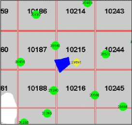
Figure 1 Location of Odder Bæk catchment in comparison to precipitation stations and the 10 km2-grids available with Danish Meteorological Institute.
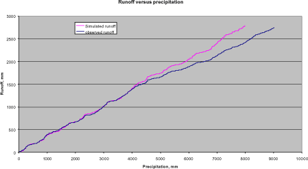
Figure 2 Runoff at the downstream station of Odder Bæk plotted against accumulated precipitation. Up to around Sept. 1994, the precipitation data stem from the local station. After this date, the precipitation file was generated as a mixture of averages of other stations. There is a clear discrepancy between the first and the last part of the curve.
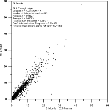
Figure 3 Precipitation station 20540 plotted against grid precipitation for grid cell 10215.
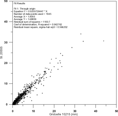
Figure 4 Precipitation station 20555 plotted against grid precipitation for grid cell 10215.
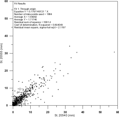
Figure 5 Precipitation station 20555 plotted against precipitation station 20540.
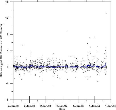
Figure 6 Daily differences between grid precipitation and station 20555.
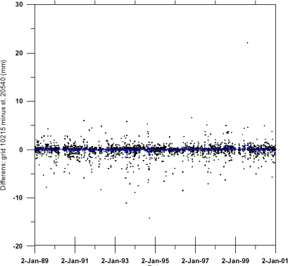
Figure 7 Daily differences between grid precipitation and station 205540.
Appendix B
1 Derivation of Parameters for the Unsaturated Zone
1.1 Hydraulic parameters
Lillebæk
The starting point for the choice of retention curves was the measured curves from the six station fields (Nielsen, 1999), earlier measured retention curves (Jensen and Madsen, 1990) and experiences from earlier calculations in Lillebæk (Sørensen and Styczen, 1994).
The division of the profiles in horizons is shown in Figure 1.
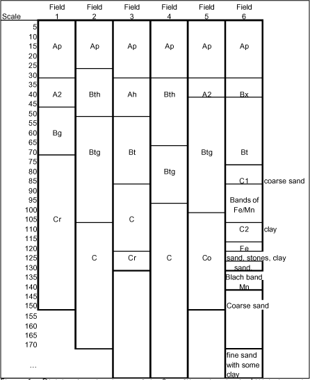
Figure 1 Division into horizons of the 6 profiles taken in the Lillebæk catchment.
The properties of the investigated profiles are shown in Table 2. All profiles have a ploughing layer of about 30 cm on top, and this is followed by Bt or Btg horizons at some depth, with higher clay content and sometimes glay features. Transformation to the clayey-material takes place between 25 and 45 cm depth.
In five out of 6 profiles, the B-horizon is limited downwards by a C-horizon with low permeability. The texture is variable; one contains significantly more silt than the others do. The last C-horizon starts in 75 cm's depth and consists of layered material, shifting between very sandy and more clayey material with a very high and very low conductivity respectively. In the 6th profile, at 1.7 m, a sandy layer with relatively high conductivity is found.
The measured retention curves for the A-horizons are difficult to use directly. shows bulk densities measured in the fields at three different occasions.
Table 1 Measurements of volume weight of the Ap-horizons of the station fields.
| Original measurements (Jensen and Madsen, 1990) |
Measurements carried out by the county of Funen, (Sørensen and Styczen, 1994) |
Recent measurements (Nielsen; 1999) |
|
| Field 1 | 1.83 | 1.45 | 1.65 |
| Field 2 | 1.69 | 1.40 | 1.75 |
| Field 3 | 1.77 | 1.46 | 1.70 |
| Field 4 | 1.64 | 1.43 | |
| Field 5 | 1.57 | 1.42 | |
| Field 6 | 1.61 | 1.38 |
It is obvious that the total porosity is very tillage dependent, and that some of the high densities recorded are unrealistic as average values of the plough layer (probably compacted by traffic). Field number 6 had fodder beets removed before the 1999-measurement, and that has influenced the density significantly.
The measured retention curves (Nielsen, 1999) of the Ap-horizons are shown in Figure 2. For modelling purposes, the curves of the Ap horizons of station 1, 2, 3, 5 and 6 have been aggregated, and saturated water content of 45 % has been assumed. This corresponds to a density of 1.4-1.45, which is a realistic value for these soils.
Curve number 4 is kept unchanged due to the fact that this soil contains more organic matter than the rest.
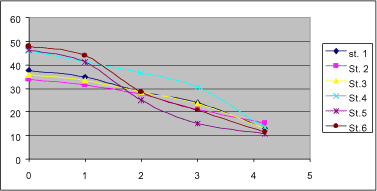
Figure 2 Retention curves of the Ap-horizons of the 6 station fields of Lillebæk.
The A2-horizon of profile 1 appears compacted, just as the Ap-horizon on the same field. Other properties are almost identical with the A2-horizon on field 5. The retention curve of St 5, A2 is therefore used to represent both horizons.
The Bh-horizon in field 2 has a volume weight of 1.74 g/cm3, which is almost inhibitive to roots, and probably not realistic as a general feature on an ordinary agricultural soil at 25 cm depth. The general properties are almost identical to Field 5, horizon Btg, and the retention properties of this soil are used to represent both horizons. On all other B-horizons, the retention data are used directly.
With respect to the C-horizons, the types have been divided into 4:
- a moraine type, which is characteristic of the C-horizon in field 1, 2 and 3, as well as the clay layer of field 6. It contains 19-23% clay and 20-25% silt.
- a silty type, which is the C-horizon in field 4. It contains more than 60% silt.
- a clayey type, which is the C-horizon of field 5. It contains about 30% clay and 20% silt.
- a sandy type, which is the lower horizon in field 6. It only contains 8% clay. The same curves are used in the sandy layer of the same field.
The hydraulic conductivities have been distributed independently of the retention curves. Generally this means that although two soils may have the same retention curve, they may differ with respect to hydraulic conductivity. As far as possible, the measured values were used as the basis for parameterisation. It was assumed that the lowest values measured represent the matrix conductivity. The geometrical average of the measured conductivity-values was then considered to be the sum of a macropore- and matrix conductivity.
Ksat (bulk) = Kmacropore + Kmatrix
Table 4-Table 8 show the estimation of conductivity values for Lillebæk. The grayed out values are the ones considered for matrix conductivity.
Table 2 Soil Texture and measured retention properties for Lillebæk.
Table 3 Soil Texture and measured retention properties for Odder Bæk.
Table 4 Measured and calculated hydraulic conductivity values for Lillebæk, Ap-horizons. Values are in mm/hr. The values for the first 3 horizons were averaged, and for the last two estimated together.
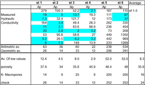
Table 5 Measured and calculated hydraulic conductivity values for Lillebæk, Second -horizons. Values are in mm/hr. Lowest values for horizon 2-4 were used to calculate matrix conductivity.
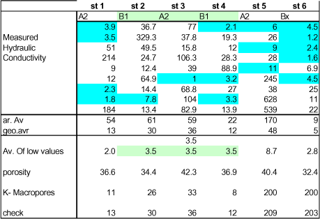
Table 6 Measured and calculated hydraulic conductivity values for Lillebæk, B/B2-horizons. Values are in mm/hr. Lowest values for horizon 2-4 were used to calculate matrix conductivity.
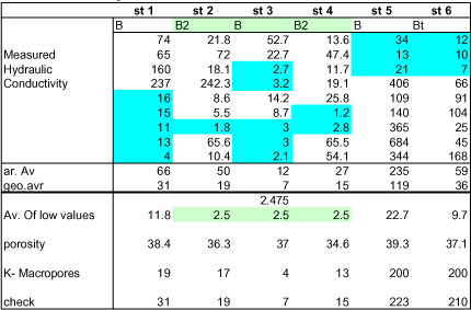
Table 7 Measured and calculated hydraulic conductivity values for Lillebæk, C-horizons. Values are in mm/hr. Lowest values for horizon 1-3 were used to calculate matrix conductivity. The corresponding conductivity of the macropores was set to 135 mm/hr.
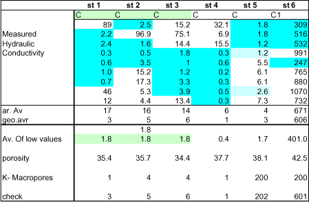
Table 8 Measured and calculated hydraulic conductivity values for Lillebæk, C2-horizons. Values are in mm/hr.
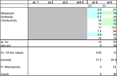
Table 9 Exponent of the unsaturated hydraulic conductivity function for the Lillebæk profiles and horizons.
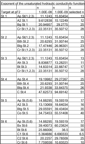
Odder Bæk
For Odder Bæk, there are clearly distinguishable soil types in the catchment according to the soil map (see Figure 3.4 in the main report. The properties of the profiles investigated are shown in Table 3. However, as there was an unclear relationship between the map information, the profile descriptions and the geological information, it was not possible to use the data directly. A different approach had to be developed.
The area is divided into 6 soil groups. The distribution of horizons is shown in Table 10 and Figure 3.
Table 10 Soil types in Odder Bæk.
| Coarse sand 1 (JB 1+3) |
Fine Sand 2 | Sand on Clay 3 | Organics on clay 4, 5 | Organics on sand 7 | |
| A | St 1 (Ap) | St 1 (Ap) | St 3 Ap | Organic | Organic |
| B | St 2 B | St 1 B | |||
| C | St 2 C | St 1 C | St 4 C (modified) | St 4 C (modified) | Station 2C |
| St 2 C2 |
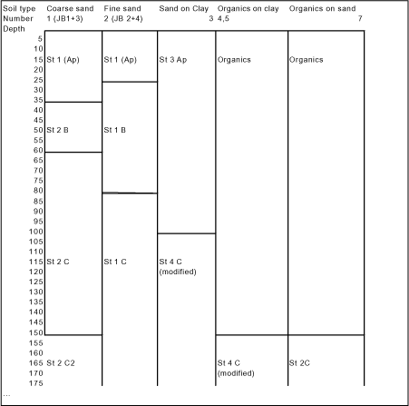
Figure 3 Depth of horizons in Odder Bæk profiles.
Originally measured retention curves were used. However, through the calibration it became clear that some of the curves were not appropriate as averages for the catchment. For the coarse sand, the measured retention curve for the C-horizon contained too much water between pF 1 and 2, meaning that the simulated groundwater variations were extremely small, and not in tune with observations. A curve was created from curve 5C and 2C (Both JB2's) that produced better correspondence with observed groundwater variations. For the same soil, the values for the B-horizon was compared to retention curves generated with the HYPRES (Wösten et al., 1998) pedotransfer-function for the same texture. The pedotransfer-values were used instead. No local measurements exist for the organic soils. The HYPRES default description was therefore used. The clay horizon (B/C) for "Sand on Clay" and "Organics on Clay" was created by comparing the curves from Station 3B and C and 4B2 and C. In the interval between saturation and pF2, it follows values of 3B, 3C and 4C, and below pF2, it follows the curve 4C. This also produced the best fit with groundwater variations. The values of the modified curves are shown in .
Table 12 Retention curves that differ from the original measurements for Odder Bæk.
| pF | Organics | 2B | 2C2 | St 4 C modified |
| 0 | 0,766 | 0,42 | 0.350 | 0,372 |
| 1 | 0,756 | 0,365 | 0.320 | 0,364 |
| 2 | 0,743 | 0,184 | 0,210 | 0,353 |
| 3 | 0,708 | 0,076 | 0,066 | 0,292 |
| 4.2 | 0,663 | 0,03 | 0,026 | 0,164 |
| 5 | 0,604 | 0,019 | 0,020 | 0,100 |
With respect to hydraulic conductivities for the unsaturated zone, the original values are shown in Table 13. The conductivities that were used for each of the horizons defined in Table 10 is shown in Table 14 together with the exponent of the hydraulic conductivity function.
Table 13 Hydraulic conductivity in Odder Bæk, average of 9 measured values, mm/hour.
| Aritmetric | Geometric | Ks | |||
| average | average | m/s | |||
| 1 | Ap | 94 | 49 | 1.36 E-5 | |
| A2 | 92 | 49 | 1,36E-5 | ||
| B | 115 | 102 | 2,83E-5 | ||
| C | 44 | 41 | 1,14E-5 | ||
| 2 | Ap | 51 | 46 | 1.27E-5 | |
| B | 222 | 196 | 5,44E-5 | ||
| B/C | 643 | 588 | 1,63E-4 | ||
| C | 824 | 767 | 2,13E-4 | ||
| 3 | Ap | 54 | 46 | 1.27E-5 | |
| B | 37 | 14 | 3.89E-6 | ||
| C | 1,9 | 1,6 | 4,44E-7 | ||
| 4 | Ap | 197 | 137 | 3.81E-5 | |
| B1 | 241 | 155 | 4,31E-5 | ||
| B2 | 6,5 | 3,8 | 1,05E-6 | ||
| C | 5,8 | 3,1 | 8,61E-7 | ||
| 5 | Ap | 102 | 78 | 2,17E-5 | |
| A/B | 76 | 72 | 2,00E-5 | ||
| B | 122 | 101 | 2,81E-5 | ||
| C | 76 | 72 | 2,00E-5 | ||
| 6 | Ap | 17 | 15 | 4,17E-6 | |
| E | 111 | 97 | 2,69E-5 | ||
| B | 24 | 20 | 5,56E-6 | ||
| C | 2,1 | 1,9 | 5,28E-7 | ||
Table 14 Calibrated values for Ks and n.
| Ks | n | |
| Station 1 (Ap) | 7.41E-06 | 11.3 |
| Station 1 (B) | 1.64E-05 | 8.28 |
| Station1(C) | 6.60E-06 | 9.55 |
| Station 2 (B) | 5.44E-05 | 12.0 |
| Station 2 (C) | 2.13E-04 | 16.0 |
| Station 2 (C2) | 2,00 E-3 | 16.5 |
| Station 3 (Ap) | 1.28E-05 | 17.0 |
| Station 4 (C) modified | 1,03 E-6 | 6 |
| Organics | 9,26E-7 | 25 |
1.2 Soil Parameters used for pesticide-relevant transformations
Pesticide simulations require specification of a number of soil parameters. The sorption values may depend on organic matter or clay content. For calculation of degradation rates, the moisture content at saturation, pF1 or pF2 are relevant. The bulk density is required for some calculations as well.
The actual values selected for these parameters are shown in Table 15 or the Lillebæk soils and in for the Odder Bæk soils.
Table 15 Carbon and clay content, bulk density and key moisture contents used to transform pesticide parameters appropriately for the different Lillebæk soils.
| Water content | ||||||||
| Soil | horizon | depth, cm | C, % | clay, % | θsat | θpF1 | θpF2 | Bulk density |
| Lillebæk, plot 1 | Ap | 0-30 | 0.99 | 16.5 | 46.4 | 41.2 | 25 | 1.42 |
| A2 | 30-40 | 1.16 | 15.9 | 36.6 | 33.6 | 27.5 | 1.68 | |
| 40-45 | 1.16 | 15.9 | 36.6 | 33.6 | 27.5 | 1.68 | ||
| Bg | 45-50 | 0.87 | 19.8 | 38.4 | 36.9 | 29.2 | 1.63 | |
| 50-70 | 0.87 | 19.8 | 38.4 | 36.9 | 29.2 | 1.63 | ||
| Cr | 70-80 | 0.12 | 19.7 | 35.4 | 34.6 | 29.8 | 1.71 | |
| -150 | 80-100 | 0.12 | 19.7 | 35.4 | 34.6 | 29.8 | 1.71 | |
| 100-105 | 0.12 | 19.7 | 35.4 | 34.6 | 29.8 | 1.71 | ||
| 105-120 | 0.12 | 19.7 | 35.4 | 34.6 | 29.8 | 1.71 | ||
| 120-170 | 0.12 | 19.7 | 35.4 | 34.6 | 29.8 | 1.71 | ||
| >170 | 0.12 | 19.7 | 35.4 | 34.6 | 29.8 | 1.71 | ||
| Lillebæk, plot 2 | Ap (25) | 0-30 | 0.99 | 18.6 | 46.4 | 41.2 | 25 | 1.42 |
| Bth (52) | 30-40 | 0.35 | 25.9 | 34.4 | 32.8 | 30.2 | 1.74 | |
| 40-45 | 0.35 | 25.9 | 34.4 | 32.8 | 30.2 | 1.74 | ||
| 45-50 | 0.35 | 25.9 | 34.4 | 32.8 | 30.2 | 1.74 | ||
| Btg | 50-70 | 0.17 | 21.7 | 36.3 | 31.8 | 28.7 | 1.69 | |
| 70-80 | 0.17 | 21.7 | 36.3 | 31.8 | 28.7 | 1.69 | ||
| 80-100 | 0.17 | 21.7 | 36.3 | 31.8 | 28.7 | 1.69 | ||
| 100-105 | 0.17 | 21.7 | 36.3 | 31.8 | 28.7 | 1.69 | ||
| C | 105-120 | 0.12 | 22.7 | 35.7 | 33.4 | 31 | 1.7 | |
| -170 | 120-170 | 0.12 | 22.7 | 35.7 | 33.4 | 31 | 1.7 | |
| >170 | 0.12 | 22.7 | 35.7 | 33.4 | 31 | 1.7 | ||
| Lillebæk. plot 3 | Ap (32) | 0-30 | 1.16 | 15.4 | 46.4 | 41.2 | 25 | 1.42 |
| Ah | 30-40 | 0.64 | 21.6 | 42.3 | 33.1 | 25.2 | 1.53 | |
| 40-45 | 0.64 | 21.6 | 42.3 | 33.1 | 25.2 | 1.53 | ||
| 45-50 | 0.64 | 21.6 | 42.3 | 33.1 | 25.2 | 1.53 | ||
| Bt (83) | 50-70 | 0.23 | 23.6 | 37 | 31.6 | 27.8 | 1.67 | |
| 70-80 | 0.23 | 23.6 | 37 | 31.6 | 27.8 | 1.67 | ||
| C | 80-100 | 0.12 | 19.4 | 34.4 | 30.4 | 27.5 | 1.74 | |
| 100-105 | 0.12 | 19.4 | 34.4 | 30.4 | 27.5 | 1.74 | ||
| 105-120 | 0.12 | 19.4 | 34.4 | 30.4 | 27.5 | 1.74 | ||
| Cr | 120-170 | 0.12 | 19.4 | 34.4 | 30.4 | 27.5 | 1.74 | |
| -200 | >170 | 0.12 | 19.4 | 34.4 | 30.4 | 27.5 | 1.74 | |
| Lillebæk. plot 4 | Ap | 0-30 | 1.8 | 17.7 | 45.9 | 41.3 | 36.6 | 1.43 |
| Bth (67) | 30-40 | 0.23 | 24.8 | 36.9 | 31.4 | 26.3 | 1.67 | |
| 40-45 | 0.23 | 24.8 | 36.9 | 31.4 | 26.3 | 1.67 | ||
| 45-50 | 0.23 | 24.8 | 36.9 | 31.4 | 26.3 | 1.67 | ||
| 50-70 | 0.23 | 24.8 | 36.9 | 31.4 | 26.3 | 1.67 | ||
| Btg (97) | 70-80 | 0.12 | 21.6 | 34.6 | 33.9 | 28.6 | 1.73 | |
| 80-100 | 0.12 | 21.6 | 34.6 | 33.9 | 28.6 | 1.73 | ||
| C | 100-105 | 0.06 | 14.4 | 37.7 | 37.6 | 35.9 | 1.65 | |
| 105-120 | 0.06 | 14.4 | 37.7 | 37.6 | 35.9 | 1.65 | ||
| 120-170 | 0.06 | 14.4 | 37.7 | 37.6 | 35.9 | 1.65 | ||
| >170 | 0.06 | 14.4 | 37.7 | 37.6 | 35.9 | 1.65 | ||
| Lillebæk. plot 5 | Ap | 0-30 | 1.22 | 14.8 | 46.4 | 41.2 | 25 | 1.42 |
| A2 (38) | 30-40 | 1.16 | 14.8 | 40.4 | 37 | 26.6 | 1.58 | |
| Btg | 40-45 | 0.29 | 24.8 | 39.3 | 39.2 | 31.4 | 1.61 | |
| 45-50 | 0.29 | 24.8 | 39.3 | 39.2 | 31.4 | 1.61 | ||
| 50-70 | 0.29 | 24.8 | 39.3 | 39.2 | 31.4 | 1.61 | ||
| 70-80 | 0.29 | 24.8 | 39.3 | 39.2 | 31.4 | 1.61 | ||
| 80-100 | 0.29 | 24.8 | 39.3 | 39.2 | 31.4 | 1.61 | ||
| Co | 100-105 | 0.17 | 30.5 | 38.1 | 37.6 | 34.1 | 1.64 | |
| -150 | 105-120 | 0.17 | 30.5 | 38.1 | 37.6 | 34.1 | 1.64 | |
| 120-170 | 0.17 | 30.5 | 38.1 | 37.6 | 34.1 | 1.64 | ||
| >170 | 0.17 | 30.5 | 38.1 | 37.6 | 34.1 | 1.64 | ||
| Lillebæk. plot 6 | Ap (28) | 0-30 | 1.22 | 17 | 46.4 | 41.2 | 25 | 1.42 |
| Bx | 30-40 | 0.46 | 21.7 | 32.4 | 31.6 | 29.1 | 1.79 | |
| Bt (75) | 40-45 | 0.17 | 20.5 | 37.1 | 36.5 | 29.8 | 1.67 | |
| 45-50 | 0.17 | 20.5 | 37.1 | 36.5 | 29.8 | 1.67 | ||
| 50-70 | 0.17 | 20.5 | 37.1 | 36.5 | 29.8 | 1.67 | ||
| Co | 70-80 | 0.06 | 4.9 | 42.5 | 36.1 | 7.5 | 1.52 | |
| 80-100 | 0.06 | 8.2 | 38.8 | 34.9 | 18.4 | 1.62 | ||
| clayey band | 100-105 | 0.06 | 14.4 | 31.5 | 30.1 | 24.6 | 1.82 | |
| 105-120 | 0.06 | 4.9 | 42.5 | 36.1 | 7.5 | 1.52 | ||
| 120-170 | 0.06 | 4.9 | 42.5 | 36.1 | 7.5 | 1.52 | ||
| Cr (250) | >170 | 0 | 8.2 | 38.8 | 34.9 | 18.4 | 1.62 | |
Table 16 Carbon and clay content, bulk density and key moisture contents used to transform pesticide parameters appropriately for the different Odder Bæk soils.
| Water content | ||||||||
| Soil | horizon | depth | C, % | clay, % | θsat | θpF1 | θpF2 | Bulk density |
| Odder Bæk | 1Ap | 0.25 | 2.32 | 6.4 | 46.7 | 39.7 | 30.8 | 1.41 |
| coarse sand on clay | 0.35 | 1.22 | 6.4 | 46.7 | 39.7 | 30.8 | 1.41 | |
| 2B | 0.6 | 0.87 | 5.7 | 42 | 36.5 | 18.4 | 1.38 | |
| 2C | 0.8 | 0.06 | 3.9 | 39.2 | 35.7 | 6.3 | 1.61 | |
| 2C | 1 | 0.06 | 3.9 | 39.2 | 35.7 | 6.3 | 1.61 | |
| 2C | 1.5 | 0.06 | 3.9 | 39.2 | 35.7 | 6.3 | 1.61 | |
| 2C2 | >1.5 | 0.09 | 4.25 | 35 | 32 | 21 | 1.655 | |
| Fine sand 2 | St1 (Ap) | 0.25 | 2.32 | 6.4 | 46.7 | 39.7 | 30.8 | 1.41 |
| St 1 B | 0.35 | 1.22 | 5.2 | 43.1 | 36.4 | 21.7 | 1.51 | |
| St 1 B | 0.6 | 0.41 | 5.2 | 43.1 | 36.4 | 21.7 | 1.51 | |
| St 1 B | 0.8 | 0.41 | 5.2 | 43.1 | 36.4 | 21.7 | 1.51 | |
| St 1. C | 1 | 0.12 | 5.1 | 39 | 33.8 | 20 | 1.62 | |
| 1.5 | 0.12 | 5.1 | 39 | 33.8 | 20 | 1.62 | ||
| >1.5 | 0.12 | 5.1 | 39 | 33.8 | 20 | 1.62 | ||
| Sand on clay | St 3 Ap | 0.25 | 2.55 | 4.7 | 49.7 | 41.8 | 30.6 | 1.33 |
| St 3 Ap | 0.35 | 1.22 | 4.7 | 49.7 | 41.8 | 30.6 | 1.33 | |
| St 3 Ap | 0.6 | 0.17 | 4.7 | 49.7 | 41.8 | 30.6 | 1.33 | |
| St 3 Ap | 0.8 | 0.17 | 4.7 | 49.7 | 41.8 | 30.6 | 1.33 | |
| St 3 Ap | 1 | 0.17 | 4.7 | 49.7 | 41.8 | 30.6 | 1.33 | |
| St 4C mod | 1.5 | 0.17 | 20.1 | 37.2 | 36.4 | 35.3 | 1.64 | |
| St 4C mod | >1.5 | 0.17 | 20.1 | 37.2 | 36.4 | 35.3 | 1.64 | |
| Soil | horizon | depth | C, % | clay, % | θsat | θpF1 | θpF2 | Bulk density |
| Organics on clay | Organic | 0.25 | 6.96 | 8 | 76.6 | 75.6 | 74.3 | 0.86 |
| Organic | 0.35 | 6.96 | 8 | 76.6 | 75.6 | 74.3 | 0.86 | |
| Organic | 0.6 | 6.96 | 8 | 76.6 | 75.6 | 74.3 | 0.86 | |
| Organic | 0.8 | 6.96 | 8 | 76.6 | 75.6 | 74.3 | 0.86 | |
| Organic | 1 | 6.96 | 8 | 76.6 | 75.6 | 74.3 | 0.86 | |
| Organic | 1.5 | 6.96 | 8 | 76.6 | 75.6 | 74.3 | 0.86 | |
| St 4C mod | >1.5 | 0.17 | 20.1 | 37.2 | 36.4 | 35.3 | 1.64 | |
| Organics on clay | Organic | 0.25 | 6.96 | 8 | 76.6 | 75.6 | 74.3 | 0.86 |
| Organic | 0.35 | 6.96 | 8 | 76.6 | 75.6 | 74.3 | 0.86 | |
| Organic | 0.6 | 6.96 | 8 | 76.6 | 75.6 | 74.3 | 0.86 | |
| Organic | 0.8 | 6.96 | 8 | 76.6 | 75.6 | 74.3 | 0.86 | |
| Organic | 1 | 6.96 | 8 | 76.6 | 75.6 | 74.3 | 0.86 | |
| Organic | 1.5 | 6.96 | 8 | 76.6 | 75.6 | 74.3 | 0.86 | |
| St. 2 C | >1.5 | 0.06 | 3.9 | 39.2 | 35.7 | 6.3 | 1.61 | |
1.3 References
Nielsen, O.H. (1999): Rapport om Jordfysiske Målinger i Landovervågningsoplandet på Fyn. November 1999. Danmarks JordbrugsForskning, Afdeling for Plantevækst og Jord.
Jensen, N.H. and Madsen, H.B. (1990): Jordprofilundersøgelse i vandmiljøovervågningsopland. Statens Planteavlsforsøg, Afdelingen for Arealdata og Krotlægning. pp 17. bilag.
Sørensen, H.R. and Styczen, M (1994): Simulation of Water and Nitrate Movements in the Lillebaek Catechment on Funen. Danish Hydraulic Institute, December, 1994. 77 pp.
Wösten, J.H.M, lilly, A., Nemes, A., and Le Bas, C. (1998): Using existing soil data to derive hydraulic parameters for simulation models in environmental studies and in land use planning.. Final Report on the European Union Funded Project. Report156. DLO-Staring Centre, Wageningen. 106 pp.
Appendix C
1 Pond Characteristics
pH: 7.6
Sediment porosity: 0.75
Sediment dry weight bulk density = 0.252000 kg/m3 = 500 kg/m3:
foc: 3.3%
Links on the internet
http://wizard.arsusda.gov/acsl/ppdb3.html
Appendix D
1 Pesticide Characteristics used for the Pond and Stream Model
1.1 Bentazone (CAS-RN: 25057-89-0)
Basic properties:
Molecular weight: 240.3 g/mol
- pKa: 3.28 (24°C) (Danish EPA), 2.92 (Syracuse); 3.3 (Pesticide Handbook)
- LogKOW: 1.41 (pH=2), 1.21 (pH=4), -0.03 (pH=6), 2,34 (pH not stated) (Syracuse); 0.77 (pH=5); -0.45 (pH=7); -0,55 (pH=9) (Pesticide Handbook). See Figure 1.
- Boiling point:
- Melting point: 141 (Danish EPA), 138 (Syracuse), 137-139 (Verscueren)
- Water solubility: 570 mg/L (pH=7, 20°C) (Danish EPA), 490 mg/L (pH=3, 20°C) (Danish EPA), 500 mg/L (Syracuse, Verschueren).
- Vapor pressure: 1.28(10-6 mmHg (pH not stated, 20 °C) (Danish EPA), 3.45(10-6 mm Hg (pH not stated, 20 °C) (Syracuse)
- Henry's constant: 7.11(10-10 atm(m3/mol (neither temperature or pH stated) (Danish EPA), 2.2(10-9 atm(m3/mol (Syracuse, estimated from water solubililty and vapor pressure at 20°C)
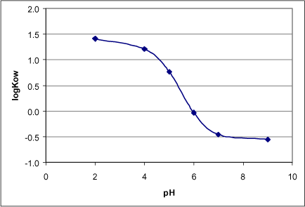
Figure 1. LogKow as a function of pH
Hydrolysis: Does not hydrolyze (HSDB, DK EPA, US EPA, Verschueren, Pesticide Handbook)
Photolysis: Is transformed by light.
Quantum yield:
Absorption spectrum:
Measured half-lives in aqueous solutions. From Danish EPA
| Half-life (h) | pH | Temp (°C) | Concentration (ppm) | Duration (h) | Light |
| 122 | 5 | 24-26 | 250 | 257 | Xenon, 850 W/m2 |
| 93 | 7 | 24-26 | 250 | 116 | Xenon, 850 W/m2 |
| 14 | 9 | 24-26 | 250 | 30.7 | Xenon, 850 W/m2 |
Biodegradation: Bentazone mineralises very slowly in water systems (Christian Helweg, 2001). The soil half-lives on primary degradation reported in the Danish EPA are between 17 days and 78 days. In sediment systems (in darkness), a very quick transformation of around 20% bentazone to an unknown metabolite was observed. After 28 days up to around 80-100% of bentazone persisted and the unknown metabolite constituted the major transformation product. No major mineralisation was observed. The results obtained in the studies of biodegradation in water-sediment systems, are not adequate to be used for determining a rate constant of the transformation of bentazone.
For the calibration of the model (only chemical analysis of the mother product was carried out in the pond experiments), a primary biodegration rate in water of bentazone 0 hr-1 is recommended, but it can be necessary to adjust the biodegradation rate, as transformation of bentazone has been observed in the water-sediment system.
Sediment-water partition coefficient (KD): The KD for the pond sediment has not been measured for bentazon. A KD-value of 0.8 L/Kg is used (average KOC=23 L/kg, a organic carbon content of 3.3% in the pond).
| Recommeded values for bentazone pKa 3.28 logKOW (at the pH of the pond) -0.5 Volatilization Henrys constant: 7.11(10-10 atm(m3/mol (undissociated part) Hydrolysis: Hydrolysis_Constant_Acid=0 Hydrolysis_Constant_Alkaline=0 Hydrolysis_Constant_Neutral=0 Photolysis: Use the photolytic half-life as a calibration parameter. Take basis in a depth averaged half-life of 28 days. Sediment-water partition coefficient (KD) Use 0.8 l/kg Retention factor in sediment 1.15 Sorption rate: 0.0363 hr-1 (g/L SS)-1 Desorption rate: 45.375 (g/L SS)-1 hr-1 Degradation rate in water column (dissolved part) 0 hr-1 Degradation rate in water column (sorped part) 0 hr-1 Degradation rate in sediment (dissolved part) 0 hr-1 Degradation rate in sediment (sorped part) 0 hr-1 |
1.2 Ioxynil (CAS-RN: 1689-83-4)
Basic properties:
Molecular weight: 370.9 g/mol
pKa: 3,96 (25°C)(Syracuse)
LogKOW: 3.51 (24°C) (Danish EPA), 6.12 (Danish EPA, Ioxynil octonoate), 3.43 (Syracuse)
Boiling point:
Melting point: 209 (Danish EPA), 212.5 (Syracuse)
Water solubility: 50 mg/L (pH=not stated, 25°C) (Danish EPA), 50 mg/L (Syracuse, Verschueren).
Vapor pressure: 5.1(10-6 mmHg (pH not stated, 25 °C) (Danish EPA), 1.38(10-7 mm Hg (pH not stated, 25 °C) (Syracuse)
Henry's constant: 5.48(10-10 atm(m3/mol (Syracuse, estimated from water solubililty and vapor pressure at 25°C)
Hydrolysis: Ioxynil octonoate is rapidly hydrolized to octanoic acid and ioxynil. Ioxynil is not expected to hydrolyze.
Photolysis: Is transformed by light.
Quantum yield (Millet et al, 1996):
| pH | Lamda range | %CH3CN | Quantuum Yield |
| 275-320 | 0.5% | (2.5 0.3)10-3 | |
| HPLC | (2.5 1.3)10-3 | ||
| 3.5 | 235-259 | 0.5 | (2.6 0.3)10-3 |
| 7.0 | 275-315 | (2.6 1.3)10-3 | |
| 7.0 | HPLC | 0.5 | (2.5 1.2)10-3 |
| 9.0 | 275-315 | 0.5 | (2.1 1.3)10-3 |
Absorption spectrum:
Biodegradation: Ioxynil mineralizes slowly in water systems (Christian Helweg, 2001). The rate of mineralization depends on the type of sediment. The rate of mineralization was measured to 0.004 d-1 (Lillebæk), 0.008 d-1 (Odderbæk) and 0.008 d-1 in a Norwegian sediment water system. Data reported in the Danish EPA indicates that no mineralization of ioxynil took place during 28 days (20°C, 10 ppm) in an aerobic sediment water suspension.
Another study reported in the Danish EPA of the transformation of radio labelled ioxynil octanoate (14C labeled in the phenylring) in a sediment/water system (concentration 50g dry sediment in 150 mL water) during 26 week shows that ioxynil octanoate is transformed/degraded with a half-life of 13.8 days (1 order rate constant = 0.05 d-1). The degradation products are ioxynil, 3-iodo-4-hydroxy-benzonitrile, 4-hydroxy-benzonitrile, CO2 and residues. After 26 week, 14CO2 accounted for 48% of the initial activity, 10.8% was found in sediment (12.6% ioxyniloctanote, 1.4% ioxynil, 1.3% 4-hydroxy-benzonitrile and 84.8 residues) and the remaining 39% was not found.
The soil half-lives on primary aerobic degradation reported in the Danish EPA are between 2.5 days and 75 days (average 7 days, std.dev. 5.5 days). The highest half-lives are observed for a soil with a very high organic matter content (34.4%).
Assuming
- a first order kinetix
- degradation takes only place for dissolved pesticide
- the maximum water holding capacity (if nothing stated) is 50%
- if notthing is stated then the water content is set to 50% of the maximum holding capacity
- KOC for ixoynil is equal to 23 L/kg
- the temperature dependency of the rate of biodegradation is assumed to follow the expression: DT50 (T) =DT50(20°C)(exp{A((T-20°C)}
where A is temperature coefficient. It is here estimated as the value giving the lowest correlation coefficient between temperature and degradation rate. A is estimated to 0.092 °C-1, corresponding to that the half-lives is 2.5 times higher for every 10°C decrease in temperature.
- The hereby calculated rate of primary degradation of dissolved pesticide at 20°C varies between 0.7 and 1.6 days-1, average 1.2 days-1, stdev. 0.3 days-1. This rate is thus between 150 and 300 times higher than the rate observed in a water phase containing suspended sediment. In case of that no data is available but for soil systems, then extrapolation from studies in sediment/water systems could be carried out by
- calculate the rate of biodegradadation in the water phase at a reference temperature
- divide this rate with 150-300 in order to get a rate of degradation in the water phasee
For the calibration of the model (only chemical analysis of the mother product was carried out in the pond experiments), a primary biodegration rate in water of ioxynil 0.004-0.008 days-1 is recommended, but it can be necessary to adjust the biodegradation rate.
Volatilization: Henrys constant: 7.11(10-10 atm(m3/mol.
Sediment-water partition coefficient (KD): The KD for the pond sediment has not been measured for ioxynil. A KD-value of 11 L/Kg is used (average KOC=335 L/kg, a organic carbon content of 3.3% in the pond).
Sorption rate:
Desorption rate:_
| Recommeded values for ioxynil pKa 3.96 logKOW (at the pH of the pond) 3.51 Volatilization Henrys constant: 5.5(10-10 atm(m3/mol (undissociated part) Hydrolysis: Hydrolysis_Constant_Acid=0 Hydrolysis_Constant_Alkaline=0 Hydrolysis_Constant_Neutral=0 Photolysis: Use the photolytic half-life as a calibration parameter. Take basis in a depth averaged half-life of 17 days. Quantuum yield: 0.0024 Sediment-water partition coefficient (KD) Use 11 l/kg Retention factor in sediment 5.75 Sorption rate: 0.0363 hr-1 (g/L SS)-1 Desorption rate: 3.3 (g/L SS)-1 hr-1 Degradation rate in water column (dissolved part) 0.0003 hr-1 Degradation rate in water column (sorped part) 0.0 hr-1 Degradation rate in sediment (dissolved part) 0.05 hr-1 Degradation rate in sediment sorped part) 0.0 hr-1 |
1.3 Pendimethalin (CAS-RN: 40487-42-1)
Basic properties:
Molecular weight: 281.3 g/mol
- pKa: 2.8 (Danish EPA). No other supporting information on that pendimethalin behaves as an acid have been found. It is quite questionable, whether the value in the Danish EPA is correct.
- LogKOW: 2.18 (Danish EPA); 5.18 (Pesticide Handbook, SRC),
- Boiling point: 330 (EPISuite)
- Melting point: 54-58°C (Pesticide Handbook, Verschueren); 56-57°C (HSDB), 56°C (SRC, EPISuite)
- Water solubility: 0.275 (25°C) (Danish EPA); 0.3 mg/L (20°C) (Pesticide Handbook, HSDB, SRC), 0.275 mg/L (25°C); (EPISuite)
- Vapor pressure: 7.1(10-6 mmHg (25°C) (Danish EPA); 1.45(10-5 mmHg (25°C) (Danish EPA); 9.38(10-6 mmHg (25°C) (Danish EPA); 3.70(10-5 mmHg (35°C) (Danish EPA); 6.0(10-5 mmHg (35°C) (Danish EPA); 2.35(10-4 mmHg (45°C) (Danish EPA); 3.0(10-5 mmHg (25°C) (Pesticide Handbook, HSDB, SRC, EPISuite)
- Henry's constant: 2.7(10-5 atm(m3/mole (25°C) (Danish EPA); 1.1(10-6 atm(m3/mole (35°C) (Danish EPA); 8.6(10-7 atm(m3/mole (HSDB, SRC)
Hydrolysis: Data in the Danish EPA indecates insignificant hydrolysis. Stable to hydrolysis (HSDB)
Photolysis: Is transformed by light. N-Propyl-3,4-dimethyl-2,6-dinitroaniline is the major degradation product (Verschueren)
Quantum yield:
Absorption spectrum:
Biodegradation: Pendimethalin mineralizes to a certain degree in water systems (Christian Helweg, 2001).
For the calibration of the model (only chemical analysis of the mother product was carried out in the pond experiments), a primary biodegration rate in water of pendimethalin 0.008 hr-1 is recommended, but it can be necessary to adjust the biodegradation rate, as transformation of bentazone has been observed in the water-sediment system.
Sediment-water partition coefficient (KD): The KD for the pond sediment was measured for pendimethalin in the pond system to be between 551 and 811 L/kg (average 702 L/kg, stdev: 140 L/kg). The average KD-value of 702 L/Kg is recommended to be used for pendimethalin sorption to the pond sediment.
| Recommeded values for pendimethalin pKa - logKOW (at the pH of the pond) Volatilization Henrys constant: 2.7(10-5 atm(m3/mole (25°C) Hydrolysis: Hydrolysis_Constant_Acid=0 Hydrolysis_Constant_Alkaline=0 Hydrolysis_Constant_Neutral=0 Photolysis: Pendimethalin degrades photolytically. Use the rate of photolysis as a calibration parameter. Start with a photolytic rate of degradation of 0.001 hr-1. Sediment-water partition coefficient (KD) 702 L/kg Retention factor in sediment 352 Sorption rate: 0.0363 hr-1 (g/L SS)-1 Desorption rate: 0.052 (g/L SS)-1 hr-1 Degradation rate in water column (dissolved part) 0.008 hr-1 Degradation rate in water column (sorped part) 0 hr-1 Degradation rate in sediment (dissolved part) 0.79 hr-1 Degradation rate in sediment (sorped part) 0 hr-1 |
1.4 Fenpropimorph (CAS-RN: 67306-03-0)
Molecular weight: 303
pKa: 6.98 (25°C) (Danish EPA). As fenpropimorph is a base, this pKa is interpreted as the base constant (gives a perfect fit to the meaured LogKow (see below).
LogKOW: 2.60 (pH=5), 4.06 (pH=7), 4.39 (pH=9), 3.60 (pH not stated), 2.44(pH not stated), 2.43(pH not stated), 2.46 (pH not stated) (all Danish EPA), 4.93 (pH not stated) (Syracuse). A KOW for the non-dissociated part respectively the dissociated part is estimted to 25376 respectively 146 using the measured logKOW, where pH has been stated.
Boiling point: > 250°C (Danish EPA), 120°C at 0.05 mmHg (Syracuse)
Melting point: <25°C (Syracuse)
Water solubility: 3.53 mg/L (pH=9-11, 20°C) (Danish EPA), 7300 (pH=4.4, 20°C) (Danish EPA). A water solubility of the non-dissociated part is thus around 3.53 mg/L and for the dissociated part around 7300 mg/L (>99% is expected to be dissociated at pH 4.4).
Vapor pressure: 1.7(10-5 mmHg (20°C, pH not stated) (Danish EPA), 3.4(10-5 (25°C, pH not stated) (Danish EPA), 2.5(10-5 (20°C, pH not stated) (Syracuse)
Henry's constant: 1.92(10-6 (atm(m3/mol) (pH=9-11, 20°C) (estimated from vapor pressure and water solubility), 9.30(10-10(atm(m3/mol) (pH=4.4, 20°C) (estimated from vapor pressure and water solubility)
Hydrolysis: Does not hydrolyze (Danish EPA)
Photolysis: Does not photolyze at pH 5 in water systems(Danish EPA), photolytic half-life in soil 30 days (Danish EPA). Biodegradation products from the soil photolysis: N-[3-(4-tert-butylphenyl)-2-methyl, 1-oxopropyl]-cis-2,6-dimethylmorpholine and N-[3-(4-tert-butylphenyl)-2-methylpropyl]-cis-2,6-dimethyl, 3-oxo-morpholine (Danish EPA).
Quantum yield:
Absorption spectrum:
KOC: 3 values of soil partition coefficient KD is reported in Danish EPA: 34.47 L/kg (pH=7.3, %OC=0.58) 73.73 L/kg (pH=7.2, %OC=2.66) and 22.62 L/kg (pH=7.0, %OC=0.51). At a pH between 7.0 and 7.3 around 34-50% of fenpropimorph is expected to be dissociated. Unfortunately, no data is reported at lower and higher pH.
An average KOC of 4384 L/kg (std.dev. 1586 L/kg) is calculated from the three data points.
The dissociated part of fenpropimorph is positively charged and is thus expected to sorp much stronger to the soil particles than the non-dissociated part. The highest KOC would thus be exptected to occur at the lowest pH. This is however not the case, as the highest KOC is obtained at pH=7.3, and the lowest KOC at pH=7.2. The KOC values, which can be derived from the Danish EPA is thus considered to be very uncertain, and care should be taken when using these data to other soil/sediment systems.
Sediment-water partition coefficient (KD):
The slurry pH of the pond sediment is 7.6, which is pretty close to the pH, at which the KOC was derived. At a pH of 7.6 around 20% is expected to be dissociated. For this system it is suggested to use the average KOC of 4384 L/kg with the awareness that is determined with a high degree of uncertainty. This give a KD of 145 L/kg (%OC=3.3%).
Sorption rate:
Desorption rate:
Biodegradation:
Metabolite 1: after derivation reaction cis-4[3-[4-(1-methoxy-carbonyl-1-methyl-ethyl)phenyl]-2-methyl-propyl]-2,6-dimethylmorpholine could be synthesized and metabolite 2: 2,6-dimethylmorpholine (Danish EPA)
BF 421-1: N-[3-(4-(2-hydroxy, 1,1-dimethyl)ethylphenyl)-2-methylpropyl]-cis-2,6-dimethyl-morpholine and BF 421-2: 2-methyl, 2-[4-(2-methyl, 3-N-cis-2,6-dimethyl-morpholine)propyl]phenyl-propionic acid. Both metabolites are found in the Rhine system and in the pond system.
RO 15-4422: [4-Aza, 6-methyl, 7-(4-tert-butylphenyl)]-2-heptanol and RO 15-4423: [3-Aza, 5-methyl, 6-(4-tert-butylphenyl)]-1-carboxyl. (Danish EPA)
Four laboratory studies of aerobic biodegradation of fenpropimorph are reported in the Danish EPA. Two of the studies are carried out with 14C-labelled fenpropimorph and it is thus probably the rate of mineralization being measured (it is not completely clear from the data reported in the database). A half-life of 20 respectively 36 days was observed in these two studies. It is not clearly stated in the two other studies, whether the measurements were carried out with 14C-labellede pesticide or if the primary degradation is measured. The reported half-lives for these two studies are 5 days respectively 13 days.
The field half-lives specified in the Danish EPA is between 9 and 181days. It is probably the half-life for the primary degradation. The observed half-lives are correlated with the temperature (correlation coefficient –0.7), time of experiment (0.5), humic content/pH (0.3/0.3), and weekly with concentration (-0.2) (see Table).
Introducing a temperature dependency of the half-life (T is the temperature i °C):
DT50 (T) =DT50(20°C)(exp{A((T-20°C)}
where A is temperature coefficient. It is here estimated as the value giving the lowest correlation coefficient with temperature and observed half-lives. A is estimated to 0.099 °C-1, corresponding to that the half-lives is 2.69 times higher for every 10°C decrease in temperature.
Correcting for the temperature effects assuming that the half-life is doubled for every 10°C decrease in temperature gives a variation in the half-lives at 20°C between 11 and 73 days. The effect of humic content (the half-lives increases with increases organic matter content due to higher sorption) and water content (the dissolved fraction increases with increasing water content causing a higher degradation rate and thus a lower half-life) is expected. The effects of pH on the field half-life is not expected, as fenpropimorph is expected to sorp stronger with decreasing pH causing a higher half-life. The effects of time of experiment on the half-life could be explained by a lag-phase due to adaption and that the degradation does not follow a complete first order degradation path-way.
The rate of biodegradation in the water phase –assuming all biodegradation takes place in the water phase – and using a KOC of 4384 L/kg – gives a biodegradation rate in water phase between 10 and 23 days-1 for the laboratory studies (a single outlier of 173 days-1) is omitted and between 7.7 and 33 days-1 for the field studies. Merging the field data and laboratory data and applying a conversion factor between 150-300 for converting soil degradation data to water column degradation data gives a degradation rate in the water column between 0.03 and 0.22 days-1, average 0.06 days-1.
| Observed DT50 | Correlation coefficients | Range in DT50 (d) |
|||||
| Concentration | Humic content | pH | Temperature | Time of experiment | Water content | ||
| -0,17 | 0,32 | 0,33 | -0,70 | 0,49 | -0,16 | 9-181 | |
| DT50 temperature corrected | -0,57 | 0,66 | 0,37 | 0,00 | 0,42 | -0,50 | 11-73 |
1.4.1 Conclusions
Volatilization: Use a Henrys constant for the non-dissociated part of 1.92(10-6 (atm(m3/mol).
Biodegradation rate: Take basis in a value of 0.06 days-1, but if required adjust the rate (can vary between 0.03 and 0.22 days-1).
Rate of photolysis:
Quantuum yield is set to 0
Rate of hydrolysis:
The three rate coefficients are set to 0.
Sediment water partition coefficient: 145 L/kg
Desorption rate:
Sorption rate:
| Recommeded values for fenpropimorph pKb 6.98 (fenpropimorph is a base) logKOW (at the pH of the pond) 1.48 Volatilization Henrys constant: 1.92(10-6 atm(m3/mol (undissociated part) Hydrolysis: Hydrolysis_Constant_Acid=0 Hydrolysis_Constant_Alkaline=0 Hydrolysis_Constant_Neutral=0 Photolysis: Use the photolytic half-life as a calibration parameter. Take basis in a rate of photolysis of 0 hr-1. A relatively high photolytic half-life is expected. Sediment-water partition coefficient (KD) Use 145 L/kg Retention factor in sediment 73.3 Sorption rate: 0.0363 hr-1 (g/L SS)-1 Desorption rate: 0.25 (g/L SS)-1 hr-1 Degradation rate in water column (dissolved part) 0.0025 hr-1 (at 20°C); temperature correction factor: 0.099 (°C)-1 Degradation rate in water column (sorped part) 0.0 hr-1 Degradation rate in sediment (dissolved part) 0.59 hr-1 (at 20°C); temperature correction factor: 0.099 (°C)-1 Degradation rate in sediment sorped part) 0.0 hr-1 |
1.5 Deltamethrin (CAS-RN: 52918-63-5)
Molecular weight: 505,205
pKa:
LogKOW: 4.6 (Pesticide Handbook), 6.2 (HSDB, Syracuse)
Boiling point:
Melting point: 99 (HSDB), 101-105°C (HSDB), 98-101°C (Verschueren)
Water solubility: 0.002 mg/L (HSDB), <0.1 mg/L (Veschueren), <0.0002 mg/L (25°C) (Pesticide Handbook)
Vapor pressure: 9.3(10-11 mmHg (25°C) (EPIWIN), 1.5(10-8 mmHg (25°C) (Syracuse, HSDB), 2(10-8 mbar (25°C) (Verschueren).
Henry's constant: 4.99(10-6 atm(m3/mole (Syracuse, estimated water solubility and vapor pressure), 3.231(10-6 atm(m3/mole (EPIWIN, estimated water solubility and vapor pressure), 3.09(10-7 atm(m3/mole, 5(10-6 atm m3/mole (estimated) (HSDB)
Hydrolysis: Does hydrolyze under alkaline conditions, but very slowly under neutral and acidic conditions. T1/2 (pH=9)=2.5 days (Pesticide Manual) – corresponds to kOH = 0.32 L/(mol(s). EPIWIN predictions: total Kb (pH>8)=6.124(10-3 L/mol s. Below pH=8 hydrolysis is expected to be indsignificant.
Photolysis: A cistrans isomerization, splitting of the ester bond, and loss of bromine occurs under UV and sunlight. The photodegradadtion half-life of deltamethrin in distilled and natural water solutions exposed to sunlight was found to range from 1 to less than 5 days (HSDB).
Quantum yield:
Absorption spectrum:
Biodegradation: Half-lives in soil: 4.9 – 6.9 weeks in sandy clay loam soil(HSDB).
Volatilization:
Sediment-water partition coefficient (KD): KOC = 46,000 – 1,630,000 L/kg (Pesticide Manual, HSDB). KOC=108,000 L/kg (EPIWIN estimated). Can only be set with a high degree of uncertainty due to the large variation in the KOC. A value of 46,000 L/kg used. This gives a KD of 1518 L/kg.
Sorption rate:
Desorption rate:
| Recommeded values for Deltamethrin pKa - logKOW (at the pH of the pond) 6.2 Volatilization Henrys constant: 5(10-6 atm(m3/mole (25°C) Hydrolysis: Hydrolysis_Constant_Acid=0 Hydrolysis_Constant_Alkaline=0.32 L/(mol(s) Hydrolysis_Constant_Neutral=0 Photolysis: Does degradade in sunlight. Use the rate of photolysis as a calibration parameter. Is expected to vary between 0.0008-0.004 hr-1. Start with a value of 0.001 hr-1. Sediment-water partition coefficient (KD) 1518 L/kg. Very uncertain Retention factor in sediment 760. Very uncertain. Can eventually be used as a calibration parameter. Sorption rate: 0.0363 hr-1 (g/L SS)-1 Desorption rate: 0.048 hr-1 (g/L SS)-1 Degradation rate in water column (dissolved part) Very difficult to estimate due to lack of precise data. A degradation rate in water column around 0.003 hr-1 is suggested to be used. Degradation rate in water column (sorped part) 0 hr-1 Degradation rate in sediment (dissolved part) Very uncertain. A value equal to 0.45 hr-1 is suggested (150 times the rate in the water column). Degradation rate in sediment (sorped part) 0 hr-1 |
1.6 Permethrin (CAS-RN: 52645-53-1)
Molecular weight: 391,29
pKa:
LogKOW: 6.1 (Pesticide Handbook), 6.5 (Syracuse, HSDB)
Boiling point: 200 °C (0.1 mmHg) (Pesticide Handbook, HSDB); >290 °C at 760 mmHg; 220 °C at 0.05 mmHg
Melting point: 34-35 (Pesticide Handbook, HSDB); cis-isomeres 63-65°C. (pesticide Handbook), 34 °C (Syracuse)
Water solubility: 0.2 mg/L (Pesticide Handbook), 0.006 mg/L (20°C) (Syracuse); 0.006 mg/L (20°C) (HSDB)
Vapor pressure: 9.75(10-9 mmHg (20°C) (Spectrum Laboratories), 2.18(10-8 mmHg (25°C) (HSDB); 0.0025 Pa (Cis)/0.0015 Pa (Trans) (HSDB)
Henry's constant: 2.51(10-8 atm m3/mole (20°C) (Spectrum Laboratories). 1.87(10-6 atm m3/mole (25°C) (Syracuse, estimated from water solubility and vapor pressure)
Hydrolysis: More stable in acid than in alkaline media (Pesticide Handbook). Hydrolyzes to 3-(2,2-dichlorovinyl)-2,2-dimethylcycloprppanecarboxylic acid and 3-phenoxbenzylalcohol. Estimated half-life at pH=9: 20 days (Spectrum Laboratories) – corresponds to kOH = 0.0336 L/(mol(s).
Photolysis: Some photochemical degradation observed in laboratory studies. Pholysis half-lives of 27.1 and 19.6 hours were determined for cis- and trans-isomers in 800 mL pond water exposed to sunlight.
Quantum yield:
Absorption spectrum:
Biodegradation: DT50 (soil, pH 4.2-7.7, o.m. 1.3-51.3) < 38 days. Field dissipaiton rate between 6 and up to 106 days reported in the ARS. An aerobic half-life of 30 days is recommended by ARS.
For the calibration of the model
Volatilization:
Sediment-water partition coefficient (KD): KOC : 19340-60870 L/kg avg: 39300 L/kg. (ARS). KOC 63100 L/kg (Spectrum Laboratories). The average value 39300 is used, giving a KD for the pond sediment : 1297 L/kg,
Sorption rate:
Desorption rate:
| Recommeded values for Permethrin pKa - logKOW (at the pH of the pond) 6.5 Volatilization Henrys constant: 1.9(10-6 atm(m3/mole (25°C) Hydrolysis: Hydrolysis_Constant_Acid=0 Hydrolysis_Constant_Alkaline=0.0336 L/(mol(s) Hydrolysis_Constant_Neutral=0 Photolysis: Does degradade in sunlight. Use the rate of photolysis as a calibration parameter. Is expected to vary between 0.0008-0.004 hr-1. Start with a value of 0.001 hr-1. Sediment-water partition coefficient (KD) 1297 L/kg. Very uncertain Retention factor in sediment 649. Very uncertain. Can eventually be used as a calibration parameter. Sorption rate: 0.0363 hr-1 (g/L SS)-1 Desorption rate: 0.028 hr-1 (g/L SS)-1 Degradation rate in water column (dissolved part) Very difficult to estimate due to lack of precise data. A degradation rate in water column around 0.08 hr-1 is suggested to be used. Degradation rate in water column (sorped part) 0 hr-1 Degradation rate in sediment (dissolved part) Very uncertain. A value equal to 11.4 hr-1 is suggested (150 times the rate in the water column). Degradation rate in sediment (sorped part) 0 hr-1 |
1.7 Esfenvalerate (CAS-RN: 66230-04-4)
Molecular weight: 419.9 g/mole
pKa: -
LogKOW: 6.22 (Danish EPA), 6.22 (25°C) (Pesticide Handbook); 6.20 (EPISuite), 6.77 (HSDB)
Boiling point: 157-167°C (Pesticide Handbook); 300°C at 37mmHg; 151-167°C (HSDB)
Melting point: 59.0-60.2°C (Pesticide Handbook, HSDB): 59.5 °C (EPISuite),
Water solubility: 0.002 mg/L (25°C) (Pesticide Handbook); 0.002 mg/L (25°C); 0.024 mg/L (25°C) (EPISuite); <0.1 mg/L (20°C)(HSDB)
Vapor pressure: 2.6(10-7 mmHg (20°C) (Danish EPA); 1.5(10-9 mmHg (25°C) (Pesticide Handbook); 1.5(10-9 mmHg (25°C); 2.8(10-7 mmHg (25°C) (HSDB); 5(10-7 mmHg (25°C) (HSDB)
Henry's constant:
Hydrolysis: Kb for pH>8: 5.49(10-3 L/(mol(s) (EPISuite). Estimated halflives of 16.3 days, 1.63 days and 3.9 hours at pH 7, 8 and 9 respectively, at 25°C (HSDB). Hydrolysis halflife (derived from data in Danish EPA): 39.2 days (pH=7, 24-26°C).
67.2 days (pH=9) (Danish EPA); 217.1 (pH=5) (Danish EPA); 129.2 (pH=5) (Danish EPA), 64.4 (pH=9) (Danish EPA).
Photolysis: The data given in the Danish EPA on photolytic degradation:
| Photolytic half-life | Conditions |
| 8.7 hours | On petri dishes precoated with a silica gel treated with 14C-esfenvalerate (0.56 microg/cm2) 25°C Artificial UV-light > 290 nm. |
| 3.3 hours | 10 ml solution with esfenvalerate were transferred to the test tube. Artificial UV-light > 290 nm. pH = 3.9 25°C |
| 5.7 hours | 10 ml solution with esfenvalerate were transferred to the test tube. Artificial UV-light > 290 nm. 25°C pH=7.2 |
| 2.5 hours | 10 ml solution with esfenvalerate were transferred to the test tube. Artificial UV-light > 290 nm. 25°C pH=9.9 |
| 19.4 hours | Artificial UV-light > 290 nm. A thin-layer plate was precoated with a silica gel treated with 14C-esfenvalerate (0.56 microg/cm2) 25°C |
| 6.8 hours | Soil (OM=3.4%; clay 18.5%; Sand: 68.5%; Silt 13.0% ) was coated on a glass plate with a thickness of ca. 500 micrometer and irradiated. Esfenvalerate in diethyl ether was evenly applied to the soil thin layer plates at a rate of approximately 0.56 microg/cm2. Artificial UV-light > 290 nm pH = 5.9 25°C |
| 2.8 hours | Soil (OM=13.2%; clay 8%; Sand: 61.5%; Silt 30.5%) was coated on a glass plate with a thickness of ca. 500 micrometer and irradiated. Esfenvalerate in diethyl ether was evenly applied to the soil thin layer plates at a rate of approximately 0.56 microg/cm2. Artificial UV-light > 290 nm pH = 4.4 25°C |
| 9.4 hours | Soil (OM=0.5%; clay 11%; Sand: 79.1%; Silt 9.9%) was coated on a glass plate with a thickness of ca. 500 micrometer and irradiated. Esfenvalerate in diethyl ether was evenly applied to the soil thin layer plates at a rate of approximately 0.56 microg/cm2. Artificial UV-light > 290 nm pH = 7.1 25°C |
| 26.4 hours (1.1 days | Soil (OM=0.5%; clay 11%; Sand: 79.1%; Silt 9.9%) was sieved and air dried and coated on thin layer plates. Esfenvalerate was then applied to the soil plates and these were exposed to outdoor conditions for 30 days. Esfenvalerate in an acetone solution was applied on the plates at a rate equivalent to 0.3 - 0.4 ng/cm2. The sunlight intensity was 520, 1640 and 130 micro W/cm2 at the begining, middle and end of the day. pH = 5.3 |
Relatively stable to heat and light (Pesticide Handbook). "Photolytic degradation may contribute to esfenvalerate's degradation on soil surfaces and water exposed to sunlight". Dominant photodegradation reaction are hdyration of the cyano group and ether cleavage in the alcohol moiety. (HSDB).
Quantum yield:
Absorption spectrum:
Biodegradation:
For the calibration of the model
Volatilization:
Sediment-water partition coefficient (KD): The following Freundlich coefficients for the soil water partitioning of esfenvalerate were found in the Danish EPA:
KD
| Kd | n | Conc (ppm). | Soil |
| 4.41 | 1.13 | 0.1; 1.0; 10.0 | OM: 0.4%; Clay: 7.0%; Sand: 84.6%; Silt: 8.4%; CEC: 9.0; Temperature: 25°C; pH=Not determined |
| 6.36 | 0.96 | 0.1; 1.0; 10.0 | OM: 1.1%; Clay: 7.2%; Sand: 81.6%; Silt: 11.2%; CEC: 7.5; Temperature: 25°C; pH=7.3 |
| 71.32 | 1.02 | 0.1; 1.0; 10.0 | OM: 2.0%; Clay: 27.5%; Sand: 19.6%; Silt: 62.8%; CEC: 20.2; Temperature: 25°C; pH=5.3 |
| 104.83 | 1.18 | 0.1; 1.0; 10.0 | OM: 1.5%; Clay: 32.4%; Sand: 52.0%; Silt: 15.6%; CEC: 5.2; Temperature: 25°C; pH=6.4 |
The KOC for esfenvalerate is estimated by estimating the average KD for each type of soil for the concentrations (0.1, 1.0, 10.0 ppm). KOC is found to vary between 1038 and 12755 L/kg, with an average value of 5547 L/kg.
Sorption rate:
Desorption rate:
| Recommeded values for Esfenvalerate pKa - logKOW (at the pH of the pond) 6.22 Volatilization Henrys constant: 7.7(10-5 atm(m3/mole (25°C) (estimated from water solubility, vapor pressure) Hydrolysis: Hydrolysis_Constant_Acid= Hydrolysis_Constant_Alkaline=0.0336 L/(mol(s) Hydrolysis_Constant_Neutral=0 Photolysis: Does degradade in sunlight. Use the rate of photolysis as a calibration parameter. Is expected to vary between 0.0008-0.004 hr-1. Start with a value of 0.001 hr-1. Sediment-water partition coefficient (KD) 1297 L/kg. Very uncertain Retention factor in sediment 649. Very uncertain. Can eventually be used as a calibration parameter. Sorption rate: 0.0363 hr-1 (g/L SS)-1 Desorption rate: 0.028 hr-1 (g/L SS)-1 Degradation rate in water column (dissolved part) Very difficult to estimate due to lack of precise data. A degradation rate in water column around 0.003 hr-1 is suggested to be used. Degradation rate in water column (sorped part) 0 hr-1 Degradation rate in sediment (dissolved part) Very uncertain. A value equal to 0.45 hr-1 is suggested (150 times the rate in the water column). Degradation rate in sediment (sorped part) 0 hr-1 |
1.8 Glyphosate (CAS-RN: 1071-83-6)
Molecular weight: 169,07
pKa:
LogKOW:
Boiling point:
Melting point:
Water solubility:
Vapor pressure:
Henry's constant:
Hydrolysis:
Photolysis:
Quantum yield:
Absorption spectrum:
Biodegradation:
Fenpropimorph acid major degradation product.
For the calibration of the model
Volatilization:
Sediment-water partition coefficient (KD):
Sorption rate:
Desorption rate:
Appendix E
1 eas sprayed with selected Pesticides in the Odder Bæk Catchment and Possibilities of Measurements of Wind Drift
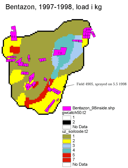
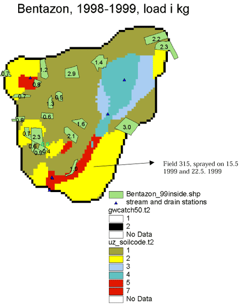
No measurements were carried out in the stream on these dates.
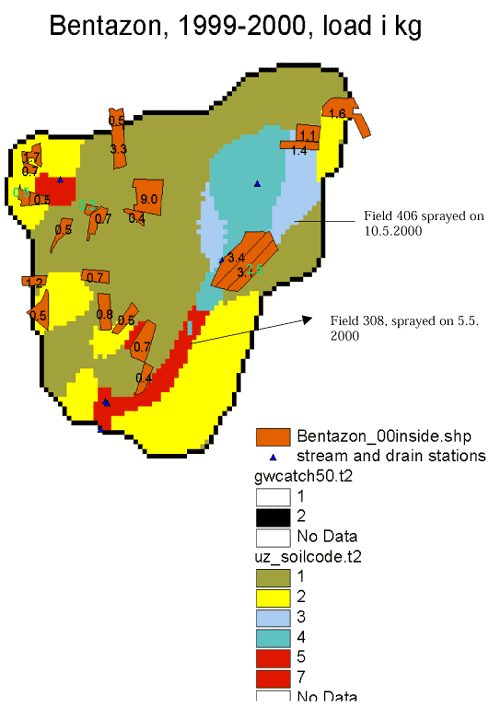
No measurements were carried out in the stream on these dates.
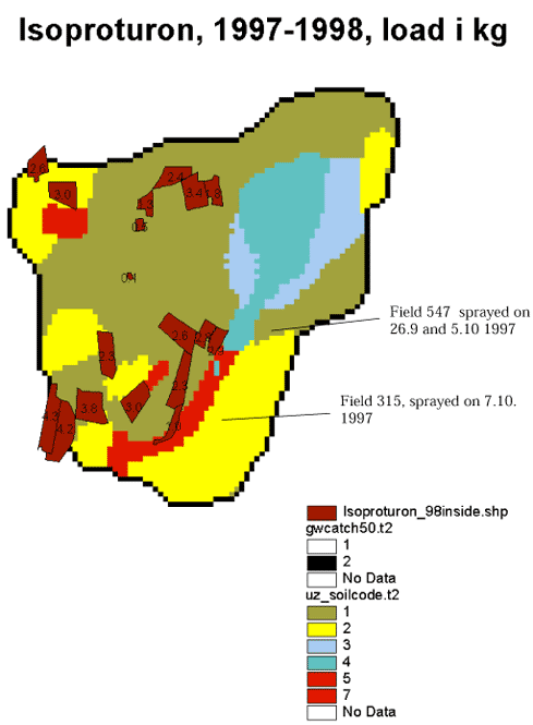
No measurements were carried out in the stream on these dates.
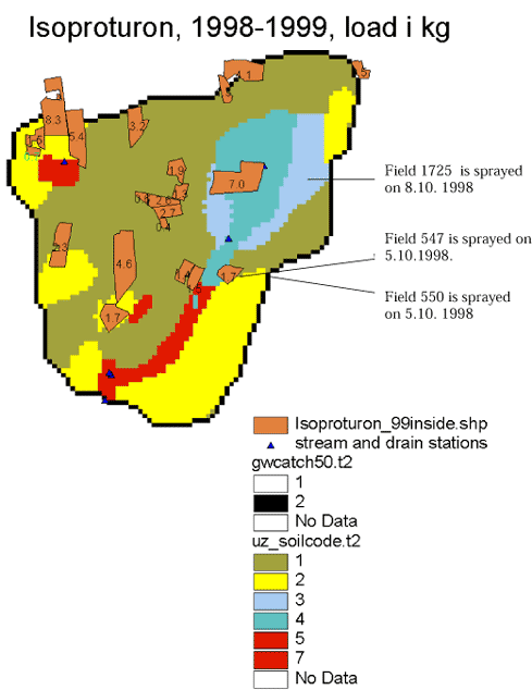
No measurements were carried out in the stream on these dates.
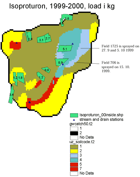
No measurements were carried out in the stream on these dates.
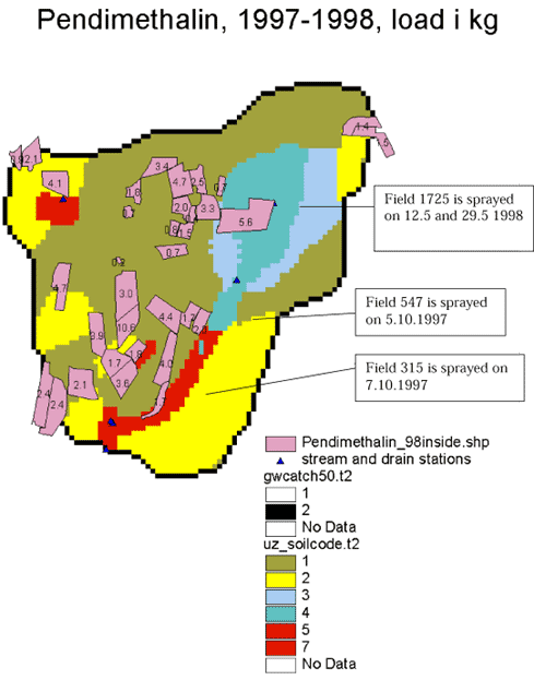
No measurements were carried out in the stream on these dates.
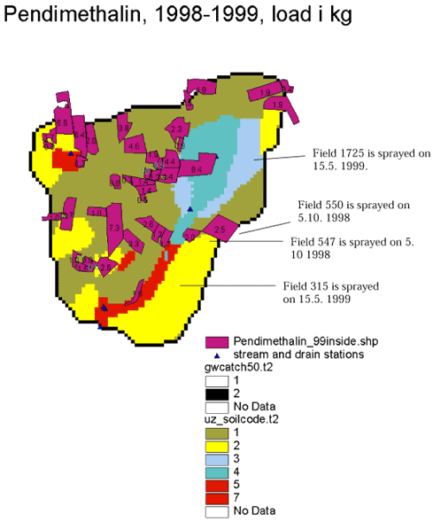
No measurements were carried out in the stream on these dates.
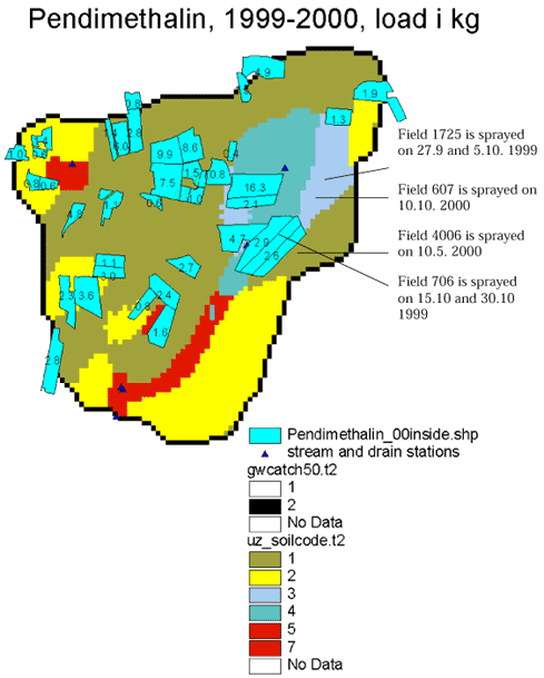
No measurements were carried out in the stream on these dates.
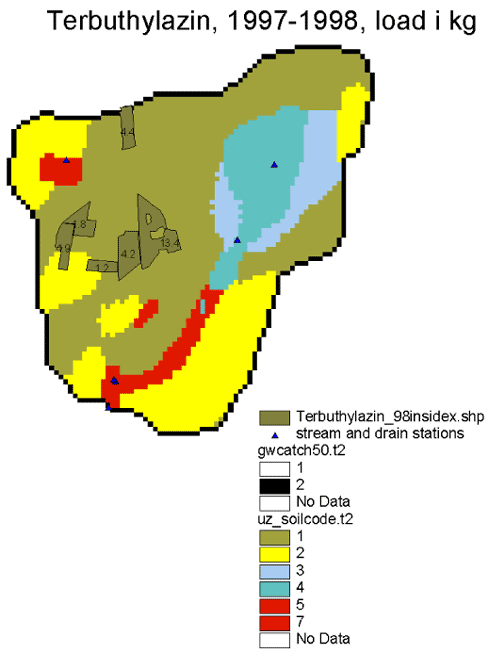
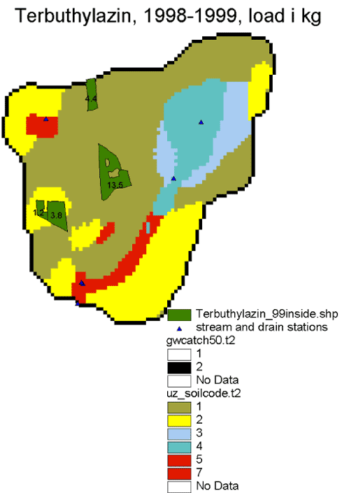
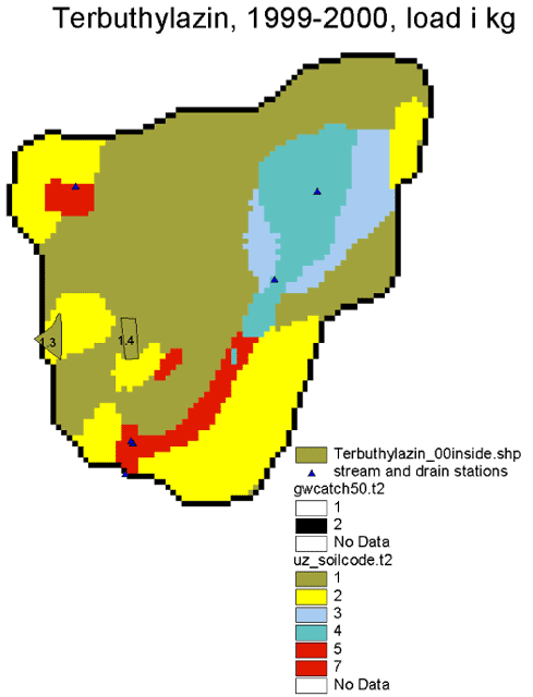
Appendix F
1 Areas sprayed with selected Pesticides in the Lillebæk Catchment and Possibilities of Measurements of Wind Drift
Bentazon, 1998
Bentazon, 1999
Bentazon, 2000
Diuron, 1998
Diuron, 1999
Diuron, 2000
Ethofumesat, 1998
Ethofumesat, 1999
Ethofumesat, 2000
Fenpropimorph, 1998
Fenpropimorph, 1999
Fenpropimorph, 2000
Loxynil, 1998
Loxynil, 1999
Loxynil, 2000
Isoproturon, 1998
Isoproturon, 1999
Isoproturon, 2000
Pendimethalin, 1998
Pendimethalin, 1999
Pendimethalin, 2000
Pirimicarb, 1998
Pirimicarb, 1999
Pirimicarb, 2000
Prochloraz, 1999
Propiconazol, 1998
Propiconazol, 1999
Propiconazol, 2000
Terbuthylazin, 1998
Terbuthylazin, 1999
Terbuthylazin, 2000
Version 1.0 November 2004, © Danish Environmental Protection Agency