|
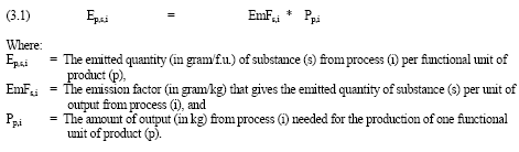
Background for spatial differentiation in LCA impact assessment - The EDIP2003 methodology 3 Acidification3.1 Introduction Authors: José Potting [16] Wolfgang Schöpp [17] Kornelis Blok [18] and Michael Hauschild [19] This Chapter is with minor modifications reproduced from an article by the same authors in the Journal for Industrial Ecology. The article is published under the title "Site-dependent life-cycle assessment of acidification" in the Journal for Industrial Ecology Vol. 2 (1998), Issue 2, p63-87. 3.1 IntroductionIn life cycle assessment (LCA) studies, generally no attention is paid to the site where an emission is released. This lack of spatial differentiation affects the relevance of the assessed impact, as was clearly demonstrated by Potting and Blok (1994, 1995). An example regarding acidification may clarify this deficiency. Copper ore contains sulphur that is released as sulphur dioxide (SO2) during the concentration of copper from the ore. The production of 1 kilogram (kg) copper is accompanied by a release of a similar amount of sulphur dioxide, of which 90% on average is captured by emission reducing measures (Potting and Blok 1993). Primary copper production takes place in Albania, Belgium and Finland. The acidifying impact per kilogram of copper is calculated to be the same for all countries if the sensitivities of the areas of deposition are not taken into account. However, sulphur emitted from Albanian copper production deposits on the highly insensitive (calcareous) areas in south Europe, while the Finnish emission deposits on the highly sensitive surrounding regions. The carrying capacity of most of the moderately sensitive West European areas is already exceeded given the lively economic activity in these regions. As a result, sulphur emitted from Belgium copper production has only moderate additional impact. Owens (1997) provides a good review of the constraints imposed on life cycle impact assessment (LCIA) by the lack of spatial and temporal differentiation in life cycle inventory (LCI). Owens is not optimistic about the possibilities of improving LCIA's accuracy in predicting non-global impacts. Other LCIA experts, however, expect that the relevance of LCIA can be enhanced considerably by the introduction into the assessment process of a few site-factors that indicate the susceptibility of the receiving areas to an impact (Potting and Blok 1994, Potting and Hauschild 1997a,b, Udo de Haes 1996, Wenzel et al. 1997). This chapter describes the framework we developed to derive such site-factors for regional impacts, and presents our results from applying this framework in the already existing RAINS model to calculate site-factors for acidification. First, some relevant principles and limitations of LCI and LCIA are outlined. This chapter primarily addresses LCA practitioners, who in general will not be familiar with the RAINS (Regional Air Pollution Information and Simulation) model and its underlying ideas and concepts. Furthermore, the model has recently adapted some important changes in response to rapid scientific developments in the field of the critical load concept. Therefore, a review is provided about the relevant parts of RAINS: emission estimates, dispersion and deposition, and the critical load concept. Results are presented and extensively discussed. Finally some main conclusions are drawn. This chapter is with minor modifications reproduced from an article by the same authors (Potting et al. 1998), which has inspired similar research activities elsewhere. These newer developments are discussed in Chapter 4. 3.2 Typical life cycle impact assessmentLife cycle inventory (LCI) quantifies the emissions per functional unit for each process in the life cycle of a product. The life cycle of an arbitrary product easily covers a multiplicity of processes, and each process may relate to a multiplicity of production sites. This makes collection of actual data for each process a time-consuming (and sometimes even impossible) activity. A regular LCI will therefore often use emission factors to approximate the emission quantities from the actual processes. An emission factor gives the emission quantity for a given substance (in grams) per unit of output (in kg) from a typical process. Spatial and temporal characteristics, and full source strength of the processes thus modelled, are lost in regular inventory analysis (and are often disregarded for the processes underlying the emission factors). To derive the emission quantity per functional unit (f.u.), the amount of process output needed for one functional unit is multiplied with the emission factor:
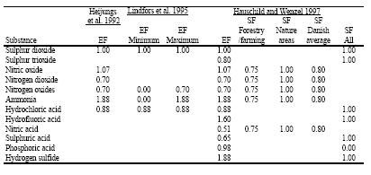
The result of LCI is a large table that lists the emission quantities per process for each substance. All emission quantities of a given substance are summed up along the life cycle, and are aggregated in the impact assessment phase (LCIA) with the summed emissions of other substances contributing to the same impact. Aggregation is based on equivalency assessment where the emitted quantity of a given substance is multiplied with an equivalency factor that relates this emission to the equivalent emission quantity of a reference substance: Table 3.1. Different sets of Characterisation or Equivalency Factors (Heijungs et al. 1992, Lindfors et al. 1995, Wenzel et al. 1997) and Site Factors (Hauschild and Wenzel 1997) for characterisation of acidification in life cycle assessment.
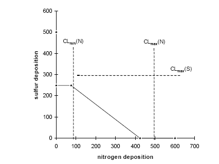
Several sets of characterisation or equivalency factors for acidification have been proposed (see Table 3.1). All these sets are based on the number of hydrogen ions that can theoretically be released from the substance (expressed in grams SO2-equivalents). The factors from Hauschild and Wenzel (1997) and Lindfors et al. (1995) distinguish roughly between different types of receiving areas but disregard emission dispersion and subsequent deposition. A more sophisticated way to deal with the current lack of spatial differentiation in LCA was proposed by Potting and Blok (1994) and Potting and Hauschild (1997a,b) in a site-dependent approach. After an acidifying substance is emitted, it is dispersed and deposited. Deposition increase together with background deposition may exceed the carrying capacity of the receiving ecosystem and result in impact. Each link in this cause/effect chain can be characterised by a set of descriptors that for acidification are specified by the geographical site where the emission takes place. This geographical site can be characterised by a site-factor that modifies the equivalence factor such that it relates the emission to the impact on its deposition areas: The only additional data needed from inventory analysis to apply Formula 3.4 is the geographical site of emission. This information is in most cases already provided by current LCI, because it is needed, for instance, to calculate the emissions from transport. 3.3 The RAINS modelRelating the site of emissions to the impact on its deposition areas is one of the key elements in the RAINS model. This model (version 7.2) has therefore been used to establish site-factors for acidification. The model was developed by the International Institute for Applied System Analysis (IIASA) in Laxenburg, Austria. RAINS is an integrated assessment model that combines information on regional emission levels with information on long-range atmospheric transport in order to estimate patterns of deposition and concentration for comparison with critical loads and thresholds for acidification, eutrophication and tropospheric ozone formation. A detailed description of the model is provided by Alcamo et al. (1990) and Amann et al. (1995). A short description of the parts of RAINS that are relevant for this chapter is given below. See Chapter 4 for a step by step illustration of the model. 3.4 Emission estimatesTypical distances between an emission source and its locations of deposition are easily several hundreds of kilometres. The geographical scale of analysis, accordingly, has to be large in order to cover most of the impact from an emission source. The RAINS model focuses therefore on the regional dimension (rather than on the local dimension) of the assessed environmental impact. On a regional scale (between 100 to 4,000 km), emissions of sulphur dioxide, nitrogen oxide and ammonia are the principal contributors to acidification. (Alcamo et al. 1990, Barret and Berge 1996) Energy consumption is the main source for emissions of sulphur dioxide and nitrogen oxides. Ammonia emissions stem predominantly from livestock farming and agricultural use of fertiliser. The 7.2 version of the RAINS model incorporates sectoral databases on energy consumption and agricultural activity for 44 regions in Europe. These primary data are based on the national forecasts of the involved countries. Several energy scenarios are provided. Current and future levels of sulphur dioxide, nitrogen oxide and ammonia are estimated by applying emission factors to these primary data. The emission factors are derived mainly from the CORINAIR 1990 emission inventory, but also from national reports and contacts with national experts. The estimated emission levels are modified according to national emission strategies. (Amann et al. 1996) The calculations in this chapter are based on the emission scenarios presented in Table 3.2 (for the year 1990) and Table 3.3 (for the year 2010). IIASA constructed these scenarios for the second interim report to the European Commission, DG-XI, entitled "Cost-effective control of acidification and ground-level ozone" (Amann et al. 1996). A comprehensive clarification of data and assumptions underlying the emission levels in Tables 3.2 and 3.3 can be found in the second interim report. The emission levels for 1990 reflect the actual situation, whereas those for 2010 are a forecast. The 1990 levels of sulphur dioxide, nitrogen oxide and ammonia are in general in good accordance with the results from the CORINAIR 1990 inventory and the EMEP database. The 2010 projections are partly based on officially announced policy targets and national emission ceilings. In addition, they build on detailed forecasts of future economic activities and application of emission control techniques in the various sectors of the economy. 3.5 Exposure assessmentThe 7.2 version of the RAINS model estimates dispersion and deposition of nitrogen and sulphur compounds on grid elements (150 km resolution), resulting from the emissions from 44 regions in Europe. The grid consists of 612 elements covering all 44 European regions, including the European part of the former Soviet Union. Total deposition for one grid element is computed by adding up the contributions from every region and the background contribution for that grid element. The dispersion and deposition estimates are based on a model developed by EMEP (co-operative Program for Monitoring and Evaluation of the long-range transmission of air pollutants in Europe). (Amann et al. 1996, Barret and Berge 1996) The EMEP model is a Lagrangian or trajectory model. In this model, an air parcel is followed on its way through the atmosphere. The EMEP model is a single layer model (see Figure 3.1). It follows air parcels along their (horizontal) travel over the two-dimensional trajectories of atmospheric motion during 96 hours preceding their arrival at a specified grid element. The (horizontal) atmospheric motion is calculated from the wind field at an altitude representing transport within the atmospheric boundary layer. (Alcamo et al. 1990, Amann et al. 1996, Barret and Berge 1996) Main inputs to and outputs from the EMEP parcels are emissions from, and wet and dry depositions on, the underlying grid elements. There is also some exchange with the free troposphere above the atmospheric boundary layer. Lagrangian models do not consider exchanges between air parcels. The size of the air parcels should be large to allow for homogenous atmospheric circumstances. In the EMEP model they measure 150 km by 150 km in the horizontal direction, and have an upper boundary that changes with the mixing height. The EMEP model considers also chemical transformations of sulphur dioxide, nitrogen oxide and ammonia within an air parcel. All chemical processes are described by ordinary first-order differential equations integrated over time. (Alcamo et al. 1990, Amann et al. 1996, Barret and Berge 1996) In Lagrangian models, all atmospheric characteristics, such as concentration and turbulence, are considered to be constant within an air parcel, and for a given time interval. The rate of transformation is determined by the parcel's characteristics at a given moment. At the end of the time interval, the situation within the air parcel changes stepwise with the product of transformation rate and the duration of the time interval. EMEP model calculations are based on input data of actual meteorological conditions that were collected every six hours for the years 1985 through 1995. For each of these years, relationships are established between sources and sinks of pollutants. The results have been averaged over 11 years and rescaled to provide the annual spatial distribution of one unit of emission. The resulting atmospheric transfer matrices are used in the RAINS model to estimate dispersion and deposition on 612 grid elements as a result of the emission in 44 regions. (Amann et al. 1996, Barret and Berge 1996) Figure 3.1. The two dimensional trajectories of atmospheric motion of a air parcel (Alcamo et al. 1990). The dispersion and deposition estimates from the EMEP model have been checked and calibrated more than once with measured annual concentrations and depositions. The EMEP estimates are therefore broadly accepted as the best available. The effect on the uncertainty in the RAINS output data were estimated to be about 10% to 25% for sulphur deposition (Alcamo et al. 1990). The use of `region to grid' atmospheric transfer matrices implicitly assumes that the spatial relative distribution of economic activities and related emissions within a region will not dramatically change in the future. It has been shown that the error introduced by this simplification is within the range of other model uncertainties. (Amann et al. 1996) Table 3.2. Total emissions for the year 1990 are given for each region (column 1) by substance (columns 2, 3 and 4). Columns 5 up to, and including column 13 represent the total area of that (column 5), the total area of ecosystem in that region (column 6), the total area of unprotected ecosystem in that region (column 7) as a percent of total area (column 8), the total area of ecosystem that gets unprotected by the total emission from that region (column 9; normalisation factors), and the acidification factors per substance for that region (columns 10, 11, 12 and 13). The acidification factors for H+ equivalents in column 13 may conditionally be used to approximate acidification factors for other acidifying substances like hydrogen chloride or hydrogen sulphide. Table 3.2. Total emissions for the year 1990 are given for each region (column 1) by substance (columns 2, 3 and 4). Columns 5 up to, and including column 13 represent the total area of that (column 5), the total area of ecosystem in that region (column 6), the total area of unprotected ecosystem in that region (column 7) as a percent of total area (column 8), the total area of ecosystem that gets unprotected by the total emission from that region (column 9; normalisation factors), and the acidification factors per substance for that region (columns 10, 11, 12 and 13). The acidification factors for H+ equivalents in column 13 may conditionally be used to approximate acidification factors for other acidifying substances like hydrogen chloride or hydrogen sulphide. Table 3.3. Total emissions for the year 2010 are given for each region (column 1) by substance (columns 2, 3 and 4). Columns 5 up to, and including column 13 represent the total area of that (column 5), the total area of ecosystem in that region (column 6), the total area of unprotected ecosystem in that region (column 7) as a percent of total area (column 8), the total area of ecosystem that gets unprotected by the total emission from that region (column 9; normalisation factors), and the acidification factors per substance for that region (columns 10, 11, 12 and 13). The acidification factors for H+ equivalents in column 13 may conditionally be used to approximate acidification factors for other acidifying substances like hydrogen chloride or hydrogen sulphide. 3.6 Effect measuresAcid deposition on forest soil may cause an imbalance of nutrients (via leaching of cations), and may mobilise toxic aluminium compounds. These changes can affect tree roots and consequently tree nutrition and water uptake. The resulting decrease in health may lower the ability of trees and other vegetation to cope with stress. (Alcamo et al. 1990) Within certain limits, forest soils are able to carry acid depositions without changing their structure and function. Acid deposition is to some extent neutralised by weathering of base cations, although it is enhanced through the uptake of base cations by vegetation. Deposition of nitrogen does not contribute to soil acidification as long as it functions as fertiliser, or if uptake and denitrification (deposition dependent) are faster than nitrogen deposition. The soil capacity to compensate for acid deposition is therefore described by the critical acid load. The critical acid load links sulphur and nitrogen deposition to the biological effects related to critical aluminium mobilisation, specified at 0.2 equivalents/m³ (Hettelingh et al. 1991, Posch et al. 1995). Figure 3.2 depicts the critical load function for a given ecosystem. There is no exceeding of the critical acid load for any combination of sulphur and nitrogen deposition lying at or below the thick line (representing the critical load function). The critical load function is defined by the maximum critical sulphur deposition (CLmax(S) at a nitrogen deposition of zero), the minimum critical nitrogen deposition (CLmin(N) where nitrogen immobilisation and uptake is equal or larger than the nitrogen deposition), and the slope of the critical load function (that reflects the linearity between nitrogen deposition and denitrification). (Hettelingh et al. 1991, Posch et al. 1995)
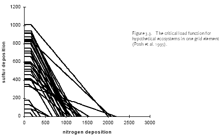
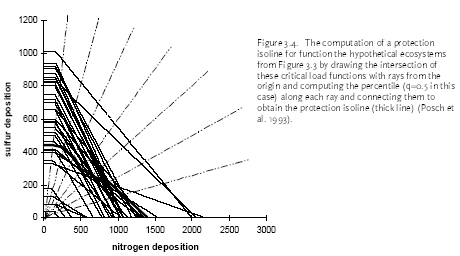
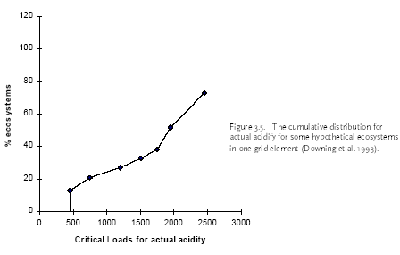
Figure 3.2. The relationship between nitrogen and some sulphur depositions and the critical loads for acidifying a hypothetical ecosystems (Posch et al. 1995). Maximum critical sulphur deposition, minimum critical nitrogen deposition, and the slope of the critical load function are characteristics of the considered ecosystem (see Figure 3.2). One EMEP grid element may contain several ecosystems, each with its own critical load function (see Figure 3.3). These critical load functions (weighed for the size of the ecosystems) can be used to construct so called protection isolines for the grid element. Such isolines consist of all combinations of S and N deposition for which a given fraction of ecosystems does not exceed critical loads, and thus in RAINS terminology is assumed to be protected against the adverse effects of acidification (see Figure 3.4) (Posch et al. 1995). The different fractions of protected ecosystem can be plotted in a two-dimensional cross-section against the critical load for actual acidity. A hypothetical example of the resulting cumulative distribution curve is shown in Figure 3.5 (Downing et al. 1993).
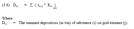
Critical load functions for acidification of forest soils have been estimated for the whole of Europe by the Co-ordination Centre for Effects at RIVM in Bilthoven, the Netherlands. In addition, critical load functions have also been established for some heath land (United Kingdom), grassland (United Kingdom and Switzerland), peatland (Switzerland and Estonia) and freshwater (Russia, Finland, Sweden, Norway, Switzerland and the United Kingdom) (Posch et al. 1995). The territory area, the total area of ecosystems, and the area of unprotected ecosystems are given for all 44 RAINS-regions in the reference situation in Table 3.2 (for the year 1990) and Table 3.3 (for the year 2010). More detailed information about critical loads and the construction of cumulative distribution functions can be found in the work of Hettelingh et al. (1991) and Posch et al. (1995). 3.7 Mathematical frameworkThe acidification impact of an emission can be expressed as the area of ecosystem that becomes unprotected as a result of that emission. The mathematical derivation of this area of ecosystem is described here. See Chapter 4 for a step by step illustration. The share of an emission from region (i) that deposits on grid element (j) is given in the RAINS model by the transport coefficient: With the help of the transport coefficient, the total deposition in grid element (j) is calculated from the emission from region (i=1 to n):
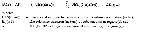
The RAINS model compares the summed deposition with the cumulative distribution curve of unprotected ecosystems in grid element (j) in order to determine the area of protected and unprotected ecosystem. The RAINS model considers regions (in most cases identical to countries), rather than the underlying separate economic activities, as sources of impact on grid elements. LCA focuses on separate processes as sources, or actually even smaller than that. LCA deals only with a fraction of the total emission from a process, namely, that emission quantity that is related to one functional unit. This fraction is generally marginal compared to the total emission from that process, and similarly, the total emission from that separate process is in general marginal compared to the total emission from one region. As a consequence, the change of deposition on grid element (j) from that particular process will also be marginal. The relationship between a change in unprotected ecosystems in grid element (j) caused by a change in emission in region (i) may be taken as linear with the transfer coefficient times the first derivative of the cumulative distribution curve for grid element (j = 1 to m), as long as the changes in deposition on grid element (j) remain marginal: The acidification factor (AFs,i in ha/tons) that directly relates a change of emission of substance (s) in region (i) to the change in unprotected ecosystems in its total deposition areas is given by: 3.8 ResultsAcidification factors have been established with the help of the RAINS model by reducing one by one the emission levels of each separate region by 10%, and then relating the result to the reference situation (the initial emission level and area of unprotected ecosystems):
A reduction of 10% has been chosen considering numerical accuracy and the functional form of the cumulative distribution curve for each grid. Calculations have been done for the years 1990 and 2010, and for sulphur dioxide, nitrogen oxide and ammonia. The reference situation and results for the year 1990 are presented in Table 3.2, and for the year 2010 in Table 3.3. 3.9 Variation of acidification factors by regionAs can be seen from Table 3.2, there are large differences among regions in the 1990 acidification factors for sulphur dioxide. The acidification factors for the southern and south-eastern European regions are in general low. This is the combined effect of the insensitivity of the receiving (calcareous) ecosystems for (changes in) acidifying depositions, and the still relatively low emission and related deposition levels in these regions. The acidification factors for the emissions from the Scandinavian and Baltic regions, and in the European part of the former Soviet Union are rather high as a result of deposition on the rather sensitive areas in these regions. The Western and Mid European regions have moderate acidification factors as a result of the large number of ecosystems that is already unprotected because of the rather high emission and related deposition levels in these regions. The 1990 acidification factors for nitrogen oxide show less pronounced differences among regions, and are in all cases lower than the acidification factors for sulphur dioxide. As long as nitrogen functions as a fertiliser, it does not contribute to acidification (note that it may contribute to eutrophication). In addition, nitrogen oxide transport extends on average longer distances than sulphur dioxide transport. This has a "smoothing" effect on the acidification factors. Given that transport distances of ammonia are relatively short, the 1990 acidification factors for this substance show sharper differences than those of nitrogen dioxide. The 2010 acidification factors (Table 3.3) show less sharp differences among regions than for those of 1990 (Table 3.2), but follow roughly the same trends described above. There are also some remarkable changes. This is as such not surprising, given that the reference emission and related deposition situation have changed considerably. As a result, the reference position on the cumulative distribution curve of unprotected ecosystems (see Figure 3.5) may also show important changes for some regions. As shown in Tables 3.2 and 3.3, the acidification factors for sea emissions can be considerable (North Sea and Baltic Sea). It is not the deposition on these sea waters from their own emissions that adds to acidification. Rather, it is the inland wind direction that prevails on sea waters that in the case of both the North and Baltic seas contributes considerably to deposition on the sensitive ecosystems of Scandinavia and the Baltic regions. The emissions from the Mediterranean Sea predominantly deposit on the rather insensitive surrounding regions, while the emissions from the Atlantic Ocean deposit only partly on (sensitive) land. The acidification factors for the Mediterranean and the Atlantic are therefore considerably less than for the North and Baltic Sea. The 1990 and 2010 acidification factors are plotted for each region in Figure 3.6 (sulphur dioxide), Figure 3.7 (nitrogen oxide) and Figure 3.8 (ammonia). The figures give insight into the changes of the acidification factors of regions from 1990 compared to 2010. The factors for Scandinavia are considerably less for 2010 than for 1990, but are still among the highest. The most striking changes occur for the Baltic regions and the former Soviet Union regions (except the Kola/Karelia region). Their factors fall considerably, which places these regions among the large group of regions with moderate to low acidification factors. Also remarkable is the increase of the ammonia factors for the West European countries. The contribution of ammonia to a change in area of unprotected ecosystem becomes apparently more important as sulphur emissions have greatly reduced. 3.10 Robustness of the marginal approachOne of the basic assumptions underlying the presented acidification factors is the marginal contribution that total emissions from separate processes in the life cycle of a product add to the total deposition on receiving grid elements. This assumption follows from a second assumption that separate processes make only a marginal contribution to the total emission from a region. This second assumption is usually true but does not apply for some exceptional cases [20]. Therefore, the robustness of the marginal approach has been investigated by pushing it beyond it limits.
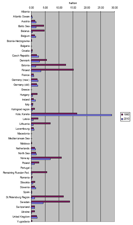
Figure 3.6. Acidification factors for sulphur dioxide in 1990 and 2010.
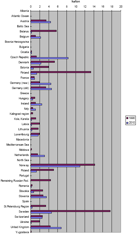
Figure 3.7. Acidification factors for nitrogen oxide in 1990 and 2010.
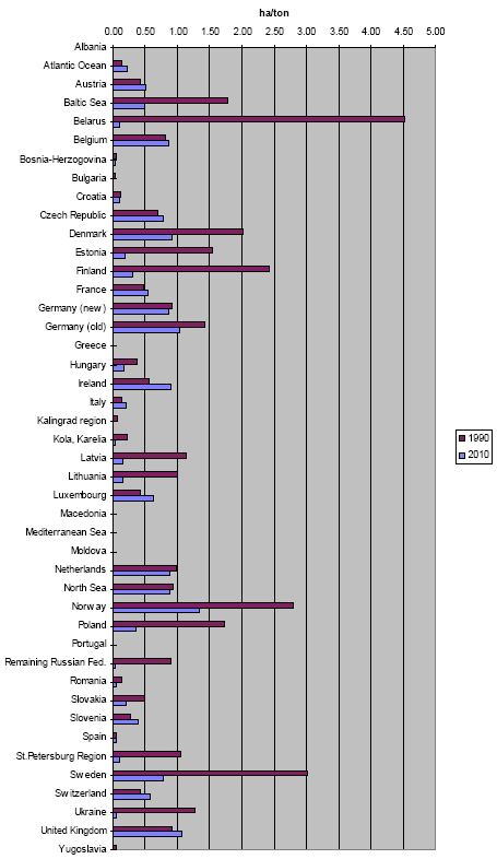
Figure 3.8. Acidification factors for ammonia in 1990 and 2010.
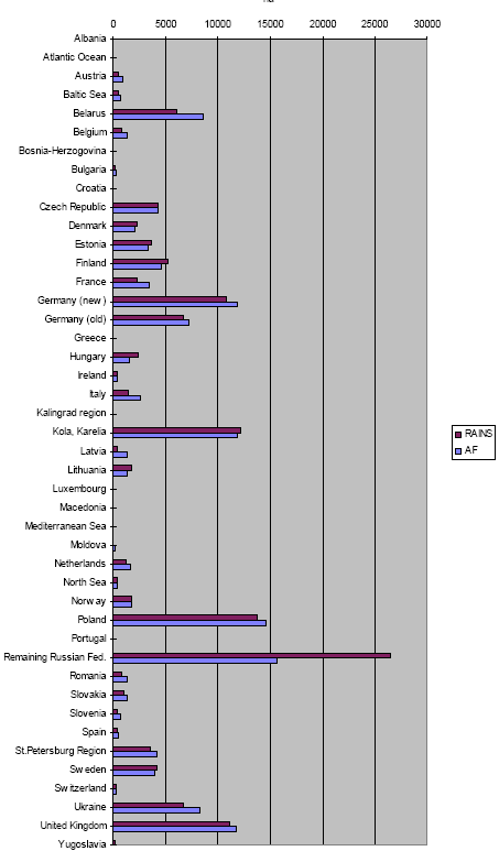
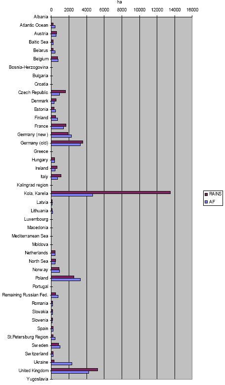
Figure 3.9. Unprotected ecosystem by the emissions from each region in 1990 predicted by multiplication with the acidification factors (AF), and predicted by the RAINS model.
Figure 3.10. Unprotected ecosystem by the emissions from each region in 2010 predicted by multiplication with the acidification factors (AF), and predicted by the RAINS model. The acidification factors have been used to estimate for each country the area of unprotected ecosystems from the total emissions from that country by multiplying the country's emission with the appropriate acidification factors. This change in area of unprotected ecosystems has also been determined with the RAINS model by reducting the total emission from each region to zero (see "Total area: unprotected ecosystem by region" in Tables 3.2 and 3.3). The results from both have been plotted in Figures 3.9 and 3.10). The accordance between both ways of prediction appears fairly good (see Figures 3.9 and 3.10). In 1990, the ratio between unprotected area predicted with the RAINS model and by use of the acidification factors is within a factor 1.1 for 23 regions, and within a factor 2 for 16 regions. These results suggest a reasonable to good stability of the estimated acidification factors for moderate changes in the reference situation. However, there are 5 regions with differences larger than a factor of 2: Latvia, Moldova, Kalingrad region, Slovenia and Yugoslavia. In 2010, there are 6 regions showing differences larger than a factor of 2: Belarus, Kola/Karelia region, Remaining Russia, St. Petersburg region, Ukraine and the Atlantic Ocean. The regions with differences larger than a factor of 2 between the RAINS estimates and the estimates with the help of the acidification factors estimates have been examined more closely. For these regions, the ratio between the decrease of unprotected ecosystems area and the emission reduction have been calculated (similar to Formula 3.13) by gradually increasing the emission reduction. The results are presented in Table 3.4. For most regions and most substances, the ratios remain quite stable with increasing emission reduction. The exceptions are restricted to SO2 and apply to Latvia and Slovenia in 1990 and the St. Petersburg region in 2010. As expected, the ratios tend to become unstable for large emission reductions of (in particular) SO2. These results again underline the reasonable to good stability of the estimated acidification factors for moderate changes in the reference situation. 3.11 Acidification factors for substances with very short lifetimesThe RAINS model focuses on the principal contributors to acidification on a regional scale (between 100 to 4,000 km): emissions of sulphur dioxide, nitrogen oxide and ammonia (Alcamo et al. 1990, Barret and Berge 1996). Close to the source (on the local scale), however, other acidifying substances like hydrochloric acid or hydrogen fluoride may also be important (Jaarsveld 1989). These other substances may fully dominate the total acidifying emissions in the life cycle of particular products. The acidification factors from these substances with very short lifetimes have been approximated on the basis of sulphur dioxide and with the help of the RAINS model in order to enable quantification of the acidifying impact from these substances. For each region, the deposition of sulphur (expressed in H+ equivalents) and the related area of unprotected ecosystems have been determined in the reference situation and for the situation in which the emissions from all regions together are reduced by 10%. The acidification factor for the emission of H+ equivalents per region has been calculated from the change in the area of unprotected ecosystems in a region, divided by the change in deposition in that region. The acidification factor for the other acidifying substances may conditionally be calculated from those for H+ equivalents, by multiplying the acidification factors for H+ equivalents with the number of H+ potentially deliverable by, and divided by the molecular mass of that substance. Approximation of the acidification factors of other acidifying substances is only acceptable under the following conditions: a substance fully deposits in the same region as where the source is located, and the deposed substance is fully leached (like sulphur) and not retained in the soil (like phosphor) or taken up by the vegetation (like nitrogen). 3.12 Application of acidification factors in LCAThe application of the acidification factors in LCIA is very simple. An emission in the product's life cycle is multiplied with the acidification factor for that region and substance to derive the estimated acidifying impact of that emission.
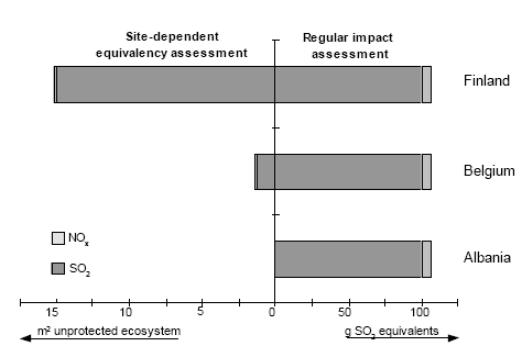
The only additional data required, the geographical site or region where an emission takes place, are in general already provided by current LCI. The earlier example on copper production in Albania, Belgium and Finland is used to demonstrate the application of, and result from the acidification factors (see Figure 3.11). Depending on the goal and scope of the study, an average "Western European" acidification factor can be used for emissions with unknown site or region, or sensitivity analysis via a worst case approach (e.g. AF-Kola/Karelia for sulphur) can be followed. Hauschild and Potting (2000), who also give a more elaborated procedure for site-dependent assessment, use the Western European average. The Guidance Document (Hauschild and Potting 2003) based on this Technical Report describes the application procedure for the acidification factors in its entirety.
Figure 3.11. The acidifying impact of 1 kg of primary cathodic copper production in Albania, Belgium, and Finland with regular equivalency assessment (Ip = Ep,s * EqFs; acidification factors from Table 3.2). For all locations similar technologies with similar emission quantities per kilogram of copper are assumed: 100 g SO2 and 10g of NOx (Potting and Blok 1993). Table 3.4. The ratios between the area of unprotected ecosystem and emission reduction for increasing reduction of emission from the given region. The established acidification factors are actually not site-factors but rather replace the product of characterisation or equivalence factor and the site-factors ( EqFs * SFs ) in Formula 3.4. They can be seen as a set of characterisation factors alternative to those in Table 3.1. The characterisation or equivalency factors in Table 3.1 pay no or only limited attention to dispersion and deposition, and the sensitivity of the receiving areas for deposition. However, one may prefer to use one's own set of characterisation or equivalency factors in combination with the acidification factors presented here. This is possible by dividing the acidification factors by the characterisation or equivalency factor for that substance. The resulting site-factors can then be used as modifier of the equivalency factor according to Formula 3.4. An optional step in LCA is normalisation. In normalisation, the assessed impact per functional unit is divided by the impact score of a reference situation (a certain region in a certain period of time) (Udo de Haes et al. 1996). A site-dependent LCIA also requires site-dependent normalisation factors (Wenzel et al. 1997). These factors have been established by comparing the reference situation of unprotected ecosystems with the situation of zero emissions from the given region. The normalisation factors are provided in Table 3.2 and 3.3 under the header "Total area: Unprotected ecosystem by Region" and are not further discussed here. 3.13 DiscussionSome remarks about the stability, feasibility and limitations of application of the established site-factors have already been made in the previous section. Here, a few additional aspects are discussed in more detail. 3.14 Uncertainties in the acidification factorsThe acidification factors are fully based on calculations with the RAINS model. The credibility of, and uncertainties in, these acidification factors are therefore strongly related to the credibility of, and uncertainties in, the model. One of the principal motives for developing the RAINS model was to provide scientific support for the negotiations in Europe under the Geneva Convention on Transboundary Air Pollution. In this role, the RAINS model as well as constituting submodules (like the EMEP atmospheric transfer matrices, and the critical loads compiled by CCE ) have gained broad scientific and political acceptance in Europe. RAINS, like all models, is a simplification of reality and will thus contain uncertainties. The uncertainties in the emission estimates, and dispersion and distribution, were already briefly discussed above. Uncertainties in critical loads have recently been analysed and shown to remain within a factor of 2 for individual ecosystems. However, these uncertainties are cancelled out to a large extent by the number of ecosystems covered (1-36',000) by most individual grid elements and Europe in total (almost 700,000) in the calculated acidification factors (Barkman 1997, Posch et al. 1997). Nevertheless, quantification of combined uncertainties in assessed impact is one of the next steps in the continuing development of the RAINS model and recommended for future update of the presented acidification factors. Although the acidification factors do contain small uncertainties, their introduction in LCIA reduces considerably the errors from the current absence of spatial differentiation. The acidification factors add resolving power of a factor thousand difference between the highest and lowest factors. The gain of information by use of these factors is thus expected to compensate fully for the introduction of new uncertainties. However, it is recommended that a future update of these acidification factors quantifies these uncertainties. The term "deposition" in this chapter refers to annual average deposition. The marginality of total emissions from separate processes justifies another assumption that implicitly underlies the presented framework: for a given moment in time, the contribution from separate processes may be regarded as marginal (though seasonal related emissions might have different deposition patterns). 3.15 Definition of the acidification factorWe defined the acidifying impact of an emission as the area of ecosystem that becomes unprotected as a result of that emission or, put another way, the area of ecosystem that is protected as a result of cutting that emission. The acidifying impact thus refers to a change in risk as a result of a change in emission. As a consequence, not reflected in the acidifying impact are those ecosystems that regardless of the change in emission remain either below or above threshold. A more sophisticated approach would have been to define the acidifying impact in a change of damage rather than in a change of risk. s68 og 68aThe critical load values for a particular ecosystem can only tell whether there is a risk of ecosystem damage Pleijel et al. (not published) advocate another approach to calculate acidification factors (or actually site-factors). They define the acidifying impact of an emission as the contribution it makes to the total deposition on an ecosystem, although they implement this by establishing the share of emission depositing on ecosystems with already exceeded critical load values (with the help of the same submodels underlying the RAINS model). This share times the emission times the relevant characterisation or equivalency factors (according to Table 3.1) gives the acidifying impact. As no calculation has been done, it is not possible to compare their results with the results of the underlying approach. However, it is possible to say something about the relevance of both approaches. Pleijel et al. consider an emission responsible for all depositions above threshold to which it contributes. This could also be interpreted in terms of a linear relation between changes in emissions and resulting damage (although damage may be expected to increase asymptotically with increasing exceeding of critical load values). Our approach considers an emission only responsible for the actual changes in risk it causes, which is useful in a strategy of risk minimisation. The most efficient way to minimise risk integrated over several ecosystems is to give priority to get (and/or keep) depositions below threshold for as many ecosystems as possible. A next sophistication would be to link this marginal approach of risk to damage. 3.16 Usefulness of the acidification factorsLCA has often been criticised for its limited ability to cope with spatial and temporal variation. Owens (1997) discusses four remedies to deal with the poor agreement between the impact as predicted by LCIA and the expected occurrence of actual impact. One of his remedies is to complement LCA with other environmental tools to address the actual relevance of the assessed impact. In this chapter we actually integrate LCA with another environmental tool. The accuracy of prediction with the resulting acidification factors is close to the maximum achievable with presently available environmental tools. Hence deposition and exceeding of critical load values must be analysed over several hundred kilometres in order to cover most of the acidifying impact from an emission. This goes far beyond the abilities of analytical tools as typically used in risk assessment and environmental impact assessment which usually have a range up to 50 km. 3.17 Conclusions and recommendationsAcidification and normalisation factors have been established for 44 regions in Europe to facilitate site-dependent LCIA of acidification. The acidification factors relate the region of emission to the impact on its deposition areas. An emission is multiplied with the acidification factor for the relevant region and substance to derive the estimated acidifying impact of the emission. The only additional required data, the geographical site or region where an emission takes place, is in general already provided by current LCI. The acidification factors show a reasonable to good level of stability of the estimated acidification factors for changes in the reference situation, and the combined uncertainties in the RAINS model are cancelled out to a large extent in the acidification factors because of the large area of ecosystems they cover. On the other hand, the acidification factors add resolving power of a factor thousand difference between highest and lowest factor. The information gain by using these factors in LCA is expected to compensate fully for the accompanying introduction of additional uncertainties. Future update of these acidification factors is recommended to quantify the uncertainties. The acidification factors presented in this chapter are based on the area of ecosystem that becomes unprotected and thus runs the risk of ecosystem damage as a result of that emission. This does not tells us whether such risk actually results in damage or how large the damage will be. The current state-of-the art in the scientific field of critical loads does not yet allow a translation of risk into damage. However, this has to be subject to future update of the established acidification factors. The framework presented here has proven capable of establishing feasible acidification factors for use in LCIA. It is desirable to extend the existing Europe set with factors for the other continents. The RAINS model provides the possibility of doing this for Asia as well. The same framework can also be used to achieve similar factors for other regional environmental impacts. The RAINS version 7.2 provides the possibility to do so for the atmospheric dimension of eutrophication in Europe, while release of a version that is extended to tropospheric ozone formation is on its way. 3.17.1 AcknowledgementResearch for this work was also supported by a Training and Mobility grant from the European Commission, and by the Danish Agency for Industry and Trade under the EUREKA project LCAGAPS. 3.18 ReferencesAlcamo, J., R. Shaw and L. Hordijk (eds.). The RAINS model of acidification. Science and strategies in Europe. Dordrecht (the Netherlands), Kluwer Academic Publishers, 1990. Amann, M., I. Bertok, J. Cofala, F. Gyarfas, C. Heyes, Z. Klimont and W. Schöpp. Cost-effective control of acidification and ground-level ozone. Second interim report to European Commission, DG-X1. Laxenburg (Austria), International Institute for Applied Systems Analysis (IIASA), 1996. Amann, M., M. Baldi, C. Heyes, Z. Klimont and W. Schöpp. Integrated assessment of emission control scenarios, including the impact of troposheric ozone. Water, air and soil pollution, Vol. 85 (1995), Issue 4, pp2595-2600. Barkman, A. Applying the critical loads concept: Constraints induced by data uncertainty. Reports in ecology and environmental engineering (report 1:1997). Lund (Sweden), Dept. of Chemical Engineering II of Lund University, 1997. Barrett, K. and E. Berge (eds.). Transboundary air pollution in Europe. Part 1: Estimated dispersion of acidifying agents and of near surface ozone. EMEP MSC-W status report (research report no. 321996). Oslo (Norway), Norwegian Meteorological Institute, 1996. Downing, R.J., J.P. Hettelingh and P.A.M. de Smet (Eds). Calculation and mapping of critical thresholds in Europe. CCE status report 1993. Bilthoven (the Netherlands), Co-ordination Centre for Effects (CCE) at the National Institute of Public Health and the Environment (RIVM), 1993. EEA. Corinair 90: Summary report no. 3, Copenhagen (Denmark), European Environmental Agency (EEA), 1996. Hauschild, M. and J. Potting. Spatial differentiation in life cycle impact assessment – the EDIP2003 methodology. Guideline from the Danish Environmental Protection Agency, Copenhagen, 2003. Hauschild, M.Z. and H. Wenzel: Environmental assessment of products. Vol. 2 - Scientific background, 565 pp. Chapman & Hall, United Kingdom, 1998, Kluwer Academic Publishers, Hingham, MA. USA. ISBN 0412 80810 2 Heijungs, R. G. Huppes, R.M. Lankreijer, H.A. Udo de Haes, A. Wegener Sleeswijk, A.M.M. Ansems, P.G. Eggels, R. van Duin and H.P. de Goede. Environmental life cycle assessment of products. Guide and backgrounds (ISBN 90-5191-064-9). Leiden (the Netherlands), Centre of Environmental Science of Leiden University, 1992. Hettelingh J-P., R.J. Downing and P.A.M. de Smet. Mapping critical loads for Europe CCE technical report no. 1. Bilthoven (the Netherlands), Co-ordination Centre for Effects (CCE) at the National Institute of Public Health and Environmental Protection (RIVM), 1991. Jaarsveld, J.A. van. Operational atmospheric transport model for priority substances; specifications and guidance for use (report no. 222501002; in Dutch). Bilthoven (the Netherlands), National Institute of Public Health and Environmental Protection (RIVM), 1989. Lindfors, L-G., K. Christiansen, L. Hoffman, Y. Virtanen, V. Juntilla, O-J. Hanssen, A. Rønning, T. Ekvall and G. Finnveden. Nordic guidelines on life cycle assessment (Nord 1995-20). Copenhagen (Denmark), Nordic Council of Ministers, 1995 Owens, W. Life cycle assessment. Constraints on moving from inventory to impact assessment. Journal of Industrial Ecology, Vol. 1 (1997), Issue 1, pp37-49. Pleijel, K., J. Altenstedt, H. Plijel, G. Lövblad, P. Grennfelt, L. Zetterberg, J. Fejes, L-G. Lindfors. A tentative methodology for the calculation of global and regional impact indicators in type-III eco-labels used in Swedish case studies. Stockholm (Sweden), Swedish Environmental Research Institute (IVL), not published. Posch, M, P.A.M. de Smet, J.P. Hettelingh, R.J. Downing (eds.). Calculation and mapping of critical thresholds in Europe. CCE status report 1995. Bilthoven (the Netherlands), Co-ordination Centre for Effects (CCE) at the National Institute of Public Health and the Environment (RIVM), 1995. Posch, M., J.P. Hettelingh, R.J. Downing, and P.A.M. de Smet (Eds). Calculation and mapping of critical thresholds in Europe. CCE status report 1997. Bilthoven (the Netherlands), Co-ordination Centre for Effects (CCE) at the National Institute of Public Health and the Environment (RIVM), 1997. Potting, J. and K. Blok. Environmental interventions from some primary and secondary materials and components in electronic products (report no. 93070; in Dutch). Utrecht (the Netherlands), Dept. of Science, Technology and Society of Utrecht University, 1993. Potting, J. and K. Blok. 1995. Life cycle assessment of four types of floor covering. Journal of Cleaner Production, Vol. 3 (1995), Issue 4, pp201-213. Potting, J. and K. Blok. Spatial aspects of life cycle impact assessment. In: Udo de Haes, H.A., A.A. Jensen, W. Klöpffer and L-G. Lindfors (eds.). Integrating impact assessment into LCA. Proceedings of the LCA symposium held at the fourth SETAC-Europe Congress, 11-14 April 1994 at the Free University of Brussels in Belgium. Brussels (Belgium), Society of Environmental Toxicology and Chemistry – Europe, 1994. Potting, J. and M. Hauschild. Predicted environmental impact and expected occurrence of actual environmental impact. Part 1: The linear nature of environmental impact from emissions in life cycle assessment. Int. Journal of Life Cycle Assessment, Vol. 2 (1997a), Issue 3, pp171-177. Potting, J. and M. Hauschild. Predicted environmental impact and expected occurrence of actual environmental impact. Part 2: Spatial differentiation in life cycle assessment by site-dependent characterisation of environmental impact from emissions. Int. Journal of Life Cycle Assessment, Vol. 2 (1997b), Issue 4, pp209-216. Potting, W. Schöpp, K. Blok and M. Hauschild. Site-dependent life-cycle assessment of acidification". Journal of Industrial Ecology Vol. 2 (1998), Issue 2, pp63-87. Udo de Haes, H.A. (ed.). Towards a methodology for life cycle impact assessment. Belgium, Brussels, Society of Environmental Toxicology and Chemistry – Europe, 1996. Wenzel, H., M.Z. Hauschild and L. Alting: Environmental assessment of products. Vol. 1 - Methodology, tools, techniques and case studies, 544 pp. Chapman & Hall, United Kingdom, 1997, Kluwer Academic Publishers, Hingham, MA. USA. ISBN 0 412 80800 5. Fodnoter [16] Institute of Product Development (IPU) in Denmark until 2000, presently at the Center for Energy and Environmental Studies IVEM, University of Groningen [17] International institute for Applied Systems Analysis (IIASA) in Austria [18] University of Utrecht, Department of Science, Technology and Society, the Netherlands [19] Institute of Product Development (IPU) in Denmark [20] The most extreme exception is Bulgaria, where two power plants determine 45% of total sulphur dioxide emission (EEA 1996), while the contribution from Bulgaria to sulphur deposition on its own area is 55% (Barret and Berge 1996). This means that these two power plants contribute almost 25% to total deposition on Bulgaria. The first assumption holds reasonable well even for this extreme case.
|