Model assessment of reductive dechlorination as a remediation technology for contaminant sources in fractured clay: Modeling tool
6 Modeling tool - case-study
- 6.1 Introduction
- 6.2 Presentation of the site
- 6.3 Results from 2D
- 6.4 Application of the modeling tool to other real cases
- 6.5 Application of the modeling tool to real cases
6.1 Introduction
In order to apply the modeling tool, some important key parameters have to be known. Hence a good geological characterization, especially concerning the fractures in the clay system, is crucial to be able to apply the model. As presented in Miljøstyrelsen [2008], the geological characterization of the clay till is often poor at the different field sites investigated and further work is needed to obtain the relevant parameters. However an extended characterization of the geology at the field site Vadsbyvej has been performed with focus on the fractures in the clay till [Christiansen and Wood, 2006]. This field site will be used to illustrate an initial application of the modeling tool. In the third phase, the model will be applied to 2-3 sites.
6.2 Presentation of the site
The part is based on site characterization of [Region Hovedstaten, 2007], a updated version of this report (with a new mass estimation) can be found in [Region Hovedstaten, 2008], but has not been used. A more detailed model of this field site will be presented in the third report of this project.
The presence of a chemical depot from 1973 resulted in soil and groundwater contamination with PCE, TCE, 1,1,1-TCA, BTEX, pesticides, acetone and isopropanol. The source is located in the upper clay till, where soil concentration up to 56 mg TCE/kg and water concentration up to 90 mg VC/L are found [Region Hovedstaten, 2007]. A sketch of the geology is shown in Figure 6.1. For more details on Vadsbyvej, see [Miljøstyrelsen, 2008] and [Region Hovedstaten, 2007].
![Figure 6.1 – Conceptualization of the local geology in the Vadsby area, from [Christiansen and Wood, 2006]](images/s055.gif)
Figure 6.1 – Conceptualization of the local geology in the Vadsby area, from [Christiansen and Wood, 2006]
6.2.1 Characterization of the clay system
Vertical fractures are not expected to extend very much deeper than 6 meters below surface (top of the saturated zone), based on the thickness of the saturated clay till and field observations. In this project, we are focusing on transport in the saturated zone, so below the fractured zone. Therefore, the clay till at this site may be considered as a block, with no vertical fractures traversing the entire depth of the till deposit. This corresponds to scenario 3, as defined in Figure 2.2 in Section 2.1.1. In such a system, the contaminant is transported by diffusion in the matrix. It is expected that some horizontal sand lenses and fractures are present in the clay till but these pathways are disregarded in this model. The physical properties of the clay till are:
- Porosity φ = 0.3
- Dry bulk density ρb = 1.96 kg/L
- Clay till thickness hclay = 10 m
6.2.2 Characterization of the source
The contamination at Vadsbyvej consists in two separate hotspots. In this report, we are focusing on hotspot 1. The source was divided into five zones, and the total mass of chlorinated ethenes is given for each zone. In this project we disregard the first zone, corresponding to the unsaturated zone and the last zone corresponding to the residual phase. Only three zones remain in the calculations, where the total mass of chlorinated ethenes is distributed among TCE, DCE and VC based on the average distribution of contaminant in the source. These total concentrations are then converted to aqueous concentrations. In the absence of field data regarding the sorption coefficient or the fraction of organic carbon, the sorption coefficients are calculated assuming foc = 1.5 % (KdTCE = 0.93 L/kg, KdDCE = 0.18 L/kg and KdVC = 0.06 L/kg). This foc value is large compare to standard value, but as explained in Section 1 and noted in Region Hovedstaden [2007], sorption on clay till is in general higher than the one calculated with the standard foc value.
The source is assumed to have a parallelepiped shape, where the length is equal to the width. The concentrations in the source are modeled as uniform concentrations (values in row Total in Table 6.2). The concentrations given in the two tables are total aqueous and sorbed concentrations and the NAPL phase is neglected.
Table 6.1 - Source zones characteristics
| Area | Depth | Total mass |
TCE | DCE | VC | TCE | DCE | VC | |
| m² | mbs | kg | kg | kg | kg | g/L | g/L | g/L | |
| Zone 1 | 100 | 5 – 10 | 56 | 42 | 11.76 | 2.24 | 0.0840 | 0.0235 | 0.0045 |
| Zone 2 | 60 | 10 – 13 | 2.6 | 1.93 | 0.54 | 0.10 | 0.0107 | 0.0030 | 0.0006 |
| Zone 3 | 20 | 13 – 15 | 4.19 | 3.14 | 0.88 | 0.17 | 0.0785 | 0.0220 | 0.0042 |
| Total | 100 | 5 – 15 | 62.8 | 47.07 | 13.18 | 2.51 | 0.0471 | 0.0132 | 0.0025 |
Table 6.2 - Aqueous concentrations in the different source zones
| aqueous TCE |
aqueous DCE |
aqueous VC |
sum | sum | |
| µg/L | µg/L | µg/L | µg/L | g/m³ | |
| Zone 1 | 39570 | 36029 | 10728 | 86328 | 86 |
| Zone 2 | 5052 | 4600 | 1370 | 11022 | 11 |
| Zone 3 | 36982 | 33673 | 10026 | 80682 | 81 |
| Total | 22174 | 20190 | 6012 | 48375 | 48 |
6.2.3 Characterization of the secondary aquifer
As shown in Figure 6.1, the clay till overlies a sand aquifer, which has the following characteristics:
- Hydraulic gradient i = 0.7 %
- Horizontal hydraulic conductivity K = 2.5*10-6 - 3.2*10-5 m/s
- Effective porosity φaq = 0.2
- Thickness b = 2.4 m
As no vertical fractures are assumed to be present in the clay till, the secondary aquifer can be considered to be confined (see Section 5.3.1). In the absence of field data, the vertical transverse dispersivity is assumed to be aTV = 0.005 m.
6.3 Results from 2D
The results from different simulations, as well as the field measurements, are summarized in Table 6.3. The details of the simulations are explained in the following sections.
Table 6.3 - Summary of model results for different configurations
| Source homogenous distributed |
Aquifer model steady state/transient |
Constant/transient boundary condition |
Concentration at B301 – 13m |
Concentration at RB1 – 39m |
Contaminant flux in aquifer |
| µg/L | µg/L | g/year | |||
| Field measurements | 151 | 0.04 | 2.7 | ||
| Homogenous | Steady-state | Constant | 225 | 225 | 6 |
| Homogenous | Transient | Constant | 225 | 0.54 | |
| Distributed | Steady-state | Constant | 170 | 170 | 4.5 |
| Distributed | Transient | Constant | 169 | 0.14 | |
| Distributed | Transient | Transient | 75 | 0.017 | |
6.3.1 Model with a homogenous source
Assuming contamination of the clay till occurred for 30 years, the total contaminant concentration (TCE + DCE + VC) distribution in the matrix is shown in Figure 6.2. The flux of the different components as well as the total flux to the underlying sand aquifer is shown in Figure 6.3. After 30 years, the total flux is around 0.6 g/year/m, which corresponds to 6 g/year (assuming a square source 10m*10m). This flux is to be compared with the measured chlorinated ethenes flux at the field site of around 2.7 g/year [Region Hovedstaden, 2007].
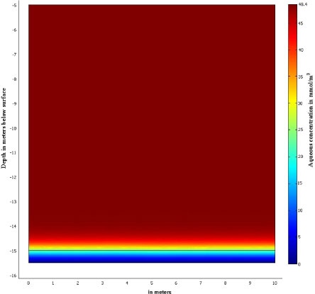
Figure 6.2 – Contaminant distribution in the clay till for a uniform source
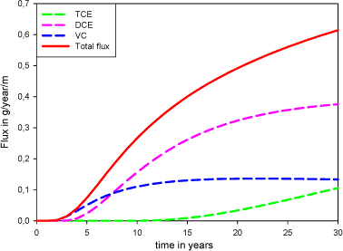
Figure 6.3 – Contaminant flux to the underlying aquifer
The simulated total contaminant flux (0.6 g/year/m) is specified at the source boundary in the underlying aquifer model. The concentration for the two cross-sections shown in Figure 6.5 (corresponding to monitoring wells B301 and RB1 at 13 and 40 meters from the source respectively, see Figure 6.4) is averaged over the whole thickness, as the two wells are fully penetrating the secondary aquifer:
CB301 = 225 µg/L
CRB1 = 225 µg/L
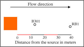
Figure 6.4 – Plan view of the source and monitoring wells
These values should be compared with the total observed concentration of chlorinated ethenes at the two wells (the summation is made on the µg/L values):
CB301 = 151 µg/L
CRB3 = 0.04 µg/L
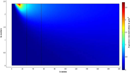
Figure 6.5 – Concentration in the aquifer for steady-state simulation
With these two simple models, it is possible to estimate the order of magnitude of the contaminant flux to the secondary aquifer as well as the concentration in the aquifer. However it has been seen that the concentration is overestimated. Therefore a more realistic model for the contaminant distribution in the source and transient character of the aquifer model is set-up in the next section.
6.3.2 Distributed source concentration and transient model
Improvement of the source model
In order to improve the accuracy, a more realistic model of the source area can be set up, where the source is divided into three zones. Inside each of these zones, the concentrations are assumed to be homogenous (see values in
Table 6.2).
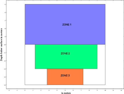
Figure 6.6 – Definition of the source's zones in the clay till
The total contaminant (TCE + DCE + VC) distribution in the matrix obtained with this heterogeneous source is shown in Figure 6.7. The three zones are clearly visible on this figure, with the highest concentrations found in zones 1 and 3.
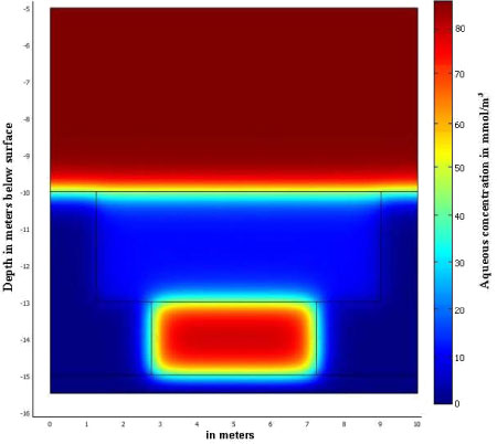
Figure 6.7 – Contaminant distribution in the clay till
The flux of the different components as well as the total flux to the underlying sand aquifer is shown in Figure 6.8. After 30 years, the total flux is around 0.45 g/year/m, which corresponds to 4.5 g/year (assuming a square source 10m*10m).
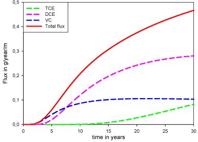
Figure 6.8 – Contaminant flux to the underlying aquifer
Improvement of the aquifer model
The low hydraulic gradient and conductivity implies a relatively low velocity in the aquifer (around 3.5 m/year), therefore the steady-state model may overestimate the concentration in the aquifer. Hence a transient model may be more appropriate for the aquifer model.
Two transient models are set-up, one with a constant flux boundary (0.45 g/year/m) and the other with a transient flux boundary condition: 0.45*t/30 g/year/m, where t is the time in years. This transient condition is a simple linear fit to the red curve in Figure 6.8. The average concentration (over the whole thickness) for the two cross-sections (corresponding to two monitoring wells) is:
CB301 = 169 µg/L
CRB1 = 0.14 µg/L for the constant boundary
CB301 = 75 µg/L
CRB1 = 0.017 µg/L for the transient boundary
The distributed source model combined with a transient aquifer model compare better the total observed concentration of chlorinated ethenes at wells B301 and RB3:
CB301 = 151 µg/L
CRB1 = 0.04 µg/L
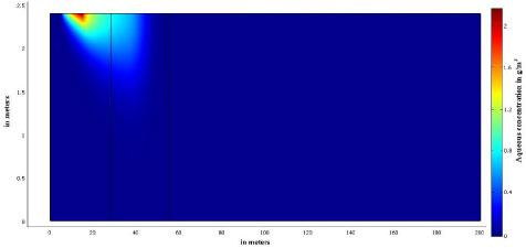
Figure 6.9 – Concentration in the aquifer at t=30 years with a constant boundary condition
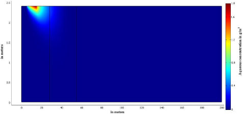
Figure 6.10 – Concentration in the aquifer at t=30 years with a transient boundary condition
The presence of the three zones in the source area does not significantly change the results. However the use of a transient model for the aquifer allows a better simulation of the concentration in the aquifer and the real extent of the plume. The model results obtained in the different configuration are summarized in Table 6.3 at the beginning of this section.
This model is a simple attempt to represent Vadsbyvej field site, and would need some improvements to be more realistic. Mainly the presence of horizontal sand lenses, observed at the field site, should be implemented in the mode, in order to have a better simulation of the contamination distribution in the source zone and hence be able to predict the future developments of this contamination zone and the contaminant flux to the aquifer.
6.4 Application of the modeling tool to other real cases
In the third phase of this project, the modeling tool developed in this report will be applied to other field sites. For the cases, where reductive dechlorination is used as remediation technology, it will be possible to verify the model accuracy. For the cases the model will be used to assess the potential of using reductive dechlorination as a remediation technology with the given field site conditions.
6.5 Application of the modeling tool to real cases
In the third phase of this project, the modeling tool developed in this report will be applied to several Danish field sites. For the cases, where reductive dechlorination is used as remediation technology, it will be possible to verify the model accuracy. For the other cases the model will be used to assess the potential of using reductive dechlorination as a remediation technology with the given field site conditions.
Version 1.0 July 2009, © Danish Environmental Protection Agency