Model assessment of reductive dechlorination as a remediation technology for contaminant sources in fractured clay: Modeling tool
5 Coupling of the “sub-models”
In this section, the two sub-models described in Sections 0 and 1 are coupled in a unique numerical model, in order to simulate transport and degradation of TCE in a single fracture – clay matrix system. The model implementation is first described and the influence of the different parameters and configurations on the results is assessed.
5.1 Theory
5.1.1 Transport equations in matrix and fracture
In the model, we will consider a set of identical vertical fractures whose axes are parallel and equally spaced (Figure 5.1). Hence the fracture network is characterized by only two parameters, the fracture aperture 2b and the fracture spacing 2B. Fracture porosity φf = b/B is generally used to characterize such fractured porous media [Freeze and McWhorter, 1997], φf ranges between 10-4 and 10-2 for typical fractured sedimentary deposits [Parker et al., 1997].
A model is constructed with the following assumptions:
- Fracture width is much smaller than its length
- Transverse diffusion and dispersion within the fracture assures complete mixing across its width at all times
- Transport within the matrix will be mainly by molecular diffusion (see Section 4.1)
- Transport along the fracture is much faster than transport within the matrix
- No adsorption on the fracture wall
Because of the symmetry of the system, we need to consider only one half of a fracture and one half of the intervening porous matrix. The transport processes in the system are described by two coupled equations (one 1D for the fracture and one 2D for the matrix), with the coupling being provided by concentration continuity along the interface.
The differential equation describing transport along the fracture is [Sudicky and Frind, 1982]:
![]()
Where Cf is the aqueous concentration in the fracture (in µmol/L), vf is the groundwater velocity in the fracture (in m/s), Df is the hydrodynamic dispersion coefficient (in m²/s), Qm is the mass transfer flux from the fracture due to diffusion at the fracture-matrix interface (in µmol/s/m²) and b is the half aperture of the fracture (in m).
![Figure 5.1 - Facture-matrix system (from [Sudicky and Frind, 1982])](images/s038a.gif)
Figure 5.1 - Facture-matrix system (from [Sudicky and Frind, 1982])
The hydrodynamic dispersivity coefficient is defined as [Fetter, 1998]:
![]()
Where αL is the longitudinal dispersivity (in m) and D* is the free diffusion coefficient in water (in m²/s).
The mass transfer flux Qm can be expessed by Fick’s first law:
![]()
Where φ is the matrix porosity, Dm is the diffusion coefficient in the matrix (see Section 4.1) and Cm is the aqueous concentration in the matrix (µmol/L).
As seen in see Section 4.1, the diffusive process in the matrix can be written:
![]()
Where Rm is the retardation factor (see Section 4.1). The two equations are coupled.
Assuming that degradation occurs only in the aqueous phase, the two transport equations are modified to include a chemical reaction rate, according to [Fetter, 1998]:
The reaction rates are as described in Section 0.
5.1.2 Determination of flow through fracture
SprækkeJAGG approach
The flow through the fracture is estimated using the conceptual model employed in SprækkeJAGG [SprækkeJAGG, 2008]: the net precipitation that falls on the land surface will flow downwards through the fractures. Hence the water flow through a single fracture can be estimated with:
![]()
Where Qf is the water flow in the fracture per unit meter (m³/year/m), I is the net precipitation rate (m/year) and 2B is the distance between two fracture (m). Based on this approach, the fracture velocity, vf, can be calculated:
![]()
This approach may be reasonable when the distance between two fractures is small, but it is unrealistic when B is large. Furthermore it can be noticed that with this definition, the flow in the fracture does not depend on its aperture.
Figure 5.2 – Definition of flow into fracture
“Cubic law” approach
In another model approach, the flow through the fracture can be estimated using the “cubic law” [McKay et al, 1998], where the volumetric flow is a function of the fracture aperture cubed:
![]()
Where i is the vertical hydraulic gradient along the fracture and Kf is the hydraulic conductivity of the fractures defined as
![]()
Where ρ is the fluid density (kg/m³), g is the gravitational acceleration (m/s²) and µ is the viscosity (Pa.s).
For a system of parallel fractures, the bulk hydraulic conductivity of the system Kb can be expressed as:
![]()
As Km << Kb, Equation can be reduced to
![]()
The bulk hydraulic conductivity can be measured at a field site with slug tests and given an estimation of the fracture spacing, the average hydraulic fracture aperture can be calculated with:
![]()
Inserting and in gives:
![]()
The equation above has a similar form as Equation , where I is replaced by Kbi.
Hence if the net precipitation rate I is equal to the bulk hydraulic conductivity Kb times the hydraulic gradient i (which is the case as long as both matrix and fractures are fully saturated and that the hydraulic conductivity of the matrix is very low), the two approaches will be equivalent. However the fracture aperture in SprækkeJAGG is not constrained by the other parameters of the systems and this can lead to unrealistic water balance in the clay till. Nevertheless it appears that the model is almost insensitive to the fracture aperture (see Section 5.2.5), so the two approaches will lead to similar results when the same water flow is applied as input with a given fracture spacing.
5.2 Single fracture/matrix model
5.2.1 Model set-up
The model domain is a rectangle which corresponds to half the matrix between two fractures. The transport equation is defined in the domain, while the transport equation is defined on the domain boundary, corresponding to the fracture location (Figure 5.3). The top and right boundaries are defined with a zero concentration gradient. The left boundary corresponds to continuity of concentration between fracture and matrix (Cm = Cf). The bottom boundary is also defined with a zero-concentration gradient, as it is assumed that the advective flux through the fracture is much more important than the diffusive flux that can be created at the bottom of the matrix (this assumption is documented in Section 5.2.3 and Appendix F).
Figure 5.3 - Model set-up
The default parameters used for this model are summarized in Table 5.1. The free diffusion coefficients are taken from [US EPA, 2008]. The sorption coefficients are average values of experiments performed at DTU Environment on clay samples (see Section 4.3.3). The matrix porosity is a typical value for clay till and the dry bulk density is calculated based on the dry density of quartz (2.65 kg/L). The fracture longitudinal dispersivity is an assumed value, based on the value used in Sudicky and Frind [1982] and Therrien and Sudicky [1996]. Finally the fracture aperture and spacing are average values from several Danish sites, where 2b varies between 30 and 3000 µm and 2B varies between 0.005 and 1 m [Christiansen and Wood, 2006].
The model verification with an analytical solution can be found in Appendix E.
Table 5.1 - Default transport parameters
| Parameters | Symbol | Expression | Value | Unit |
| Net recharge | I | 0.1 | m/year | |
| Fracture spacing | 2B | 0.3 | m | |
| Fracture aperture | 2b | 7*10-4 | m | |
| Water velocity in fracture | vf | I*2B/(2b) | 43 | m/year |
| Sorption coefficient TCE | Kd_TCE | 1 | L/kg | |
| Sorption coefficient DCE | Kd_DCE | 0.7 | L/kg | |
| Sorption coefficient VC | Kd_VC | 0.3 | L/kg | |
| Dry bulk density | ρb | 2.65*(1- φ) | 1.8 | kg/L |
| Matrix porosity | φ | 0.33 | - | |
| Matrix tortuosity | τ | φ | 0.33 | - |
| Retardation factor TCE | R_TCE | 1+ρb*Kd_TCE/ φ | 6.5 | - |
| Retardation factor DCE | R_DCE | 1+ρb*Kd_DCE/ φ | 4.8 | - |
| Retardation factor VC | R_VC | 1+ρb*Kd_VC/ φ | 2.6 | - |
| Longitudinal dispersivity in fracture | αL | 0.1 | m | |
| Free diffusion coef TCE | D*_TCE | 0.020 | m²/year | |
| Free diffusion coef DCE | D*_DCE | 0.022 | m²/year | |
| Free diffusion coef VC | D*_VC | 0.026 | m²/year | |
| Fracture dispersion coef TCE | Df_TCE | αL*vf+D*_TCE | 4.3 | m²/year |
| Fracture dispersion coef DCE | Df_DCE | αL*vf+D*_DCE | 4.3 | m²/year |
| Fracture dispersion coef VC | Df_VC | αL*vf+D*_VC | 4.3 | m²/year |
| Matrix diffusion coefficient TCE | Dm_TCE | D*_TCE*τ | 0.0065 | m²/year |
| Matrix diffusion coefficient DCE | Dm_DCE | D*_DCE*τ | 0.0074 | m²/year |
| Matrix diffusion coefficient VC | Dm_VC | D*_VC*τ | 0.0087 | m²/year |
5.2.2 Model outputs
An example of the model output for a simple case is explained. The default parameters are used and no degradation is assumed. The model simulates the flushing of the contaminant out of the matrix, by a flow of clean water in the fracture. The initial condition is defined with a uniform contaminant concentration in the whole matrix (for the influence of the initial conditions on the results, see Appendix G). The contaminant distribution changes with time are shown in Figure 5.4. The model is set up as shown in Figure 5.3. Each strip in Figure 5.4 represents a clay block of width 0.15 meter. The fracture is located on the left hand edge of each strip. Results show that the matrix is “cleaned” from the top-left corner to the bottom-right. Clean water enters the fracture (at the top left) and a concentration gradient is formed, resulting in counter diffusion from the matrix into the fracture. The cleaning starts at the top of the matrix where rain water enters. The water then becomes more contaminated as it flows downwards along the fracture. The contaminant concentration in the water flowing from the fracture outlet is shown in Figure 5.5, as well as the change in the total contaminant mass (total mass of contaminant divided by initial mass). It takes around 250 years to flush all contaminant out of the matrix and to reduce significantly the contaminant concentration at the fracture outlet. This long time scale is due to the very slow transport of the contaminant in the matrix, as it is controlled by molecular diffusion. Similar time scale has been reported in Reynolds and Kueper [2002] and Falta [2005].
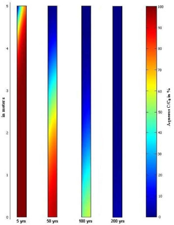
Figure 5.4 - Contaminant distribution in the matrix for different times. Each strip represents a clay block of width 0.15 meter (corresponding to 0.3 meters between fractures). No degradation
Figure 5.5 - Concentration at the fracture outlet (red - left axis) and total mass remaining in the system (blue – right axis). No degradation
5.2.3 Advective/Diffusive transport through fracture and matrix
The diffusive flux which can be created at the bottom of the matrix is assessed and compared with the advective contaminant flux at the fracture outlet, for different fracture aperture/fracture spacing configurations. In scenario 1, all contaminant leaves the system through the fracture outlet (as a zero-concentration gradient boundary is defined at the bottom of the matrix), while for scenario 2, a zero concentration boundary is defined at the bottom of the matrix, allowing contaminant to leave the system by diffusion. The conceptual models resulting from these two scenarios are shown in Figure 5.6.
Figure 5.6 - Conceptual models for the two transport scenarios
In both configurations, the flux through the matrix is minor, but differences increase when the fracture spacing is reduced, from 9% for 2B = 1m and up to 23 % for 2B = 0.005 m. An example of the contaminant fluxes for fracture spacing 2B = 0.05m is shown in Figure 5.7, where the diffusive flux is less than 20 % of the total contaminant flux.
Figure 5.7 – Flux at the output of the system in scenario 2 (for 2b = 10-4 m and 2B = 0.05 m)
Although the diffusive flux can represent up to 25 % of the total flux, it does not seem to change the model results, in term of total contaminant flux from the system and the contaminant distribution in the matrix. These results are obtained by using the transport coefficients of TCE. It is expected that the diffusive flux would be more important in the case of VC, as the diffusion coefficient is higher. Nevertheless it is assumed that the total contaminant flux will also remain the same. Therefore it was decided to use only scenario 1, where the only flux out of the system is the contaminant flux through the fracture outlet. More results and details can be found in Appendix F.
5.2.4 Degradation scenarios
As explained in Section 4.3.4, the results from field samples and literature studies have shown dechlorination may occur in a reaction zone near the high permeability sand zone (fractures), but no biomass transport or growth is expected deep within the clay matrix. Hence different scenarios need to be considered relative to degradation location:
- No degradation occurs in the system
- Degradation occurs only in the high permeable zone, i.e. the fractures
- A reaction zone is formed at the clay – fracture interface, where degradation is also taking place
- Degradation in the whole matrix
The last scenario is not likely to be realistic but is used to assess a “best case” relative to degradation.
In the absence of literature data, the degradation zone is assumed to be extended up to 0.05 m inside the clay matrix, corresponding to observations at Rugårdsvej field site. However the biomass growth in this reaction zone is restricted by pore size limitations [Lima and Sleep, 2007] and cannot be simulated in the same way as the biomass growth in the fracture. For the simplicity of the model, the biomass will be assumed to be constant both in the fracture and matrix, with a concentration of 108 cells/L, this concentration corresponds to values measured in the field after injection [Miljøstyrelsen, 2008].
These four scenarios are applied to the base case configuration with the transport parameters in Table 5.1, while the parameters relative to chlorinated solvents dechlorination are taken from Table 3.2 in Section 3.4.1. Finally a homogenous initial aqueous TCE concentration of 100 mmol/m³ is applied (equal to 13139 µg/L).
Figure 5.8 – Remaining total contaminant (TCE+DCE+VC+ETH) mass in the system for the four degradation scenarios
Figure 5.9 – TCE concentration at the fracture outlet for the three degradation scenarios
The scenario with degradation in the fracture only does not differ much from the scenario without degradation, especially concerning the mass removal rate in the system. This is due to the fact that the contaminant downward transport in the fracture, controlled by the groundwater velocity, is much higher than the degradation rate. Therefore the contaminant has no time to be degraded once it has reached the fracture (from counter diffusion from the matrix) and the production of daughter products (DCE and VC) is very limited (see Figure 5.10 - left). On the contrary in the presence of a reaction zone at the matrix – fracture interface, daughter products are formed (see Figure 5.10 - middle) and the mass removal occurs significantly faster (see Figure 5.8). As expected, under the assumption of degradation in the whole matrix, the mass removal is much faster. Ethene concentration is not displayed on the graphs but is produced by VC reductive dechlorination.
Figure 5.10 – TCE, DCE and VC concentrations at the fracture outlet for the three degradation scenarios (compared with TCE for the case without degradation)
Finally, looking at the total chlorinated solvents concentration (TCE + DCE + VC, as ethene is a non-toxic compound) at the fracture outlet for the four different scenarios (see Figure 5.11), the peak concentration in case of degradation takes place several years after the beginning of remediation. This is because of the fact that the daughter products can move more easily from the matrix than TCE, as they have higher diffusion coefficients and lower retardation factors (see Table 5.1). Once formed in the matrix, the daughter products can therefore reach the fracture faster than TCE. This peak concentration has not been noted in the literature, because the same diffusion and sorption coefficients for different compounds have been applied [Sun and Buscheck, 2003].
Figure 5.11 – Total chlorinated concentration (TCE + DCE + VC) at the fracture outlet for the four scenarios
5.2.5 Sensitivity analysis
A sensitivity analysis is performed on the independent parameters of the model, using the transport and degradation parameters from the base case scenario and applying the third degradation scenario (degradation in the fracture and in the reaction zone in the matrix). Each parameter is varied by +/- 20%. In order to compare the different simulations, the initial concentration is corrected in order to maintain the same initial total mass in the system (158 mmol).
By comparing the time to remove 90 % of the initial contaminant mass, it appears that the most sensitive parameters are the matrix porosity, the net recharge, the fracture spacing and the TCE sorption coefficient, while the least sensitive are the fracture aperture and longitudinal dispersivity in fracture. More detailed results can be found in Appendix I.
Table 5.2 - Sensitivity index for variation of +/- 20% of the parameters (transport parameters in orange and degradation parameters in green)
| Parameter | M<10% Mini |
| Matrix porosity | 55.0 |
| Net recharge | 52.5 |
| Fracture spacing | 42.5 |
| Sorption coefficient TCE | 35.0 |
| Sorption coefficient DCE | 20.0 |
| Specific yield | 20.0 |
| Initial biomass | 20.0 |
| Exponent p | 10.0 |
| Max growth rate DCE | 10.0 |
| Half velocity coefficient DCE | 7.5 |
| Sorption coefficient VC | 5.0 |
| Max growth rate TCE | 5.0 |
| Max growth rate VC | 5.0 |
| Fracture aperture | 0.0 |
| Longitudinal dispersivity in fracture | 0.0 |
5.3 Aquifer model
5.3.1 Presentation of model
The aquifer model aims at simulating the contaminant fate in a high permeability aquifer located under the clay system. In this model the clay system acts as a contamination source for the aquifer. The aquifer is represented by a vertical cross-section, assuming a groundwater flow in one horizontal direction. The model considers two-dimensional steady flow modeled with a two-dimensional advection and dispersion transport equation. Furthermore, considering the long time scale resulting from the clay system model (several hundreds of years) compared with the relatively fast transport time in the groundwater, the transport model is assumed to be at steady state (the flux from the source is assumed to change very slowly compared to the residence time in the aquifer).
For a clay system with vertical fractures down to the bottom, the aquifer can be considered as a leaky aquifer and the conceptual model with the main parameters is shown in Figure 5.12.
Figure 5.12 – Conceptual aquifer model for sand aquifer located under the clay system
W is the source width
K is the aquifer hydraulic conductivity
I is the recharge rate
φaq is the aquifer porosity
The hydraulic model is described by
![]()
which is subject to the boundary conditions:
However in the clay model it was assumed that all water flows down in the fractures, the recharge flow is here distributed with width (see top boundary definition in equation). This is reasonable given the mixing of the water at the top boundary.
The groundwater velocity is obtained using Darcy’s Law:
![]()
The contaminant transport model is given by
![]()
with
![]()
where
![]()
In such system, the model transport is insensitive to the longitudinal dispersivity αL [Prommer et al., 2006], so the dispersion tensor reduced to:
![]()
The transport model is subject to the initial and boundary conditions
Where Cf,out is the contaminant concentration at the fracture outlet (results from the clay system model).
The clay layer source is defined as a specified-flux condition to ensure a proper contaminant mass balance [Van Genuchten and Alves, 1982]. As a result, the concentration at the top boundary is not equal to the concentration at the bottom of the clay system (concentration at the fracture outlet), but all of the contaminant that leaves the clay source enters the aquifer.
For clay system with no vertical fractures, the aquifer can is confined and the recharge rate I = 0 m/year. In this case the flow and transport equations remain the same, but the boundary condition at the source is changed to:
Where Cm is the concentration in the clay matrix.
5.3.2 Model outputs
This model is used to assess the maximal concentration along a cross-section at a certain distance L from the source (Caq,L,max). The main output from this model is the dilution factor df, which is defined as the ratio between the maximum concentration in the aquifer at the distance L and the concentration at the fracture outlet (in case of fracture), or the ratio between the maximum concentration in the aquifer at the distance L and the contaminant diffusive flux through the matrix (when there is no vertical fracture):
The distance from the source to the point of compliance (POC) is defined in Denmark as one year of groundwater transport (and maximum 100 m from the source) as specified in “Oprydning på forurenede lokaliteter” [Miljøstyrelsen, 1998]. In order to have the parameter L (distance between the middle of the source to the measurement point) independent of the other model parameters (K, I, hydraulic gradient, etc…), L is defined to 100 m (and not as one year of transport).
An example of the model output is given for the following parameters:
- Hydraulic conductivity K = 2000 m/year (=6.3*10-5 m/s)
- Recharge rate I = 200 mm/year
- Hydraulic gradient i = 2 %
- Effective porosity φaq = 0.3
- Vertical transverse dispersvity αT = 0.005 m
- Source width W = 30 m
- Cfract, out = 100 mmol/m³
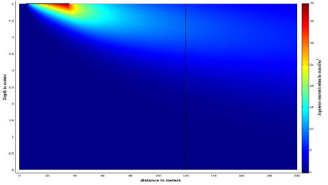
Figure 5.13 - Contaminant concentration in the aquifer at steady-state
The contaminant concentration in the aquifer reaches a maximum value of 39 µmol/L, but decreases fast along the flow line, and is less than 10 % of the fracture concentration at 100 meters from the source (see Figure 5.14).
Figure 5.14 - Dilution factor along the cross-section at 100 m from the source
The concentration distribution in the aquifer is a function of the “flow factor”, defined as the ratio of the recharge rate (I) and the mean specific discharge (=K*i).
The sensitivity analysis performed shows in addition to the flow factor, the model is sensitive to the source width and the vertical transverse dispersivity. The detailed results can be found in Appendix K.
5.4 Improving the modeling tool
This modeling tool was developed to characterize the main processes and the key parameters controlling the transport and degradation in a fractured clay till. With a single fracture – clay matrix model it was possible to assess the clean-up times for different configurations and degradation scenarios. However this model is still relatively simple and could be improved by the addition of other processes, notably in the dechlorination model. The introduction of biomass growth and decay could be interesting, even if it is possible to assume that a steady-state is reached relatively fast. Furthermore the limiting substrate condition and substrate concentration could be implemented, resulting in a more realistic modeling of the real system behavior. As explained in Section 3.1, the fermentation process, production of electron donor (here generally hydrogen) from the fermentation for the injected substrate, is also an important process in the system. The geometry of the model could also be improved by taking into account the presence of horizontal fractures, sand layers and sand lenses and considering heterogeneous fracture networks, which are closer to the real cases. Finally some studies need to be done in case the advective transport in the clay matrix can not be neglected, for example in the present of a high sand content in the clay till.
Version 1.0 July 2009, © Danish Environmental Protection Agency