Model assessment of reductive dechlorination as a remediation technology for contaminant sources in fractured clay: Modeling tool
4 Transport in the clay matrix
In this section, a model for contaminant transport in the clay matrix is developed. The model is applied to experimental data from a field site at Rugårdsvej.
4.1 Theory
Transport of the contaminant in the clay matrix is a very important process relative to risk assessment and remediation. The clay will act as a long-term contaminant source and the transport in this low permeability layer is often the limiting factor for remediation. Transport in low permeability layer, such as clay, is in most of the cases controlled by molecular diffusion, as advection/dispersion mechanisms are negligible because of the low permeability. The relative contribution of advection/dispersion and diffusion to solute transport can be evaluated with the Peclet number [Bear, 1979]:
![]()
Where v is the average flow velocity (m/s), L is the characteristic length of the system (m) and D* is the molecular diffusion coefficient in the considered liquid (here water) (m²/s). In the studied system, the average flow velocity is defined by Darcy’s law:
![]()
Where Km is the clay matrix hydraulic conductivity (m/s), i is the vertical hydraulic gradient through the clay matrix and φ is the matrix porosity.
For such systems, the characteristic length L can be defined as the thickness of the clay layer.
To insure the predominance of the molecular diffusion, the Peclet number should be smaller than 1 [Bear, 1972]. Given a free diffusion coefficient of 6.23*10-10 m²/s (corresponding to diffusion of TCE in water at 10°C, see Table 4.2), a porosity of 0.3, this condition corresponds to:
![]()
The matrix hydraulic conductivity for clay till is in the range 10-9 – 10-11 m/s in Denmark [Jørgensen et al., 1998], and the thickness can vary between 1 and 10 meters. Hence the hydraulic gradient should be smaller than 1 to insure Pe < 1, for Km = 10-9 m/s and L = 10 m (limit case). This high limit value for hydraulic gradient shows that the assumption of solute transport controlled by molecular diffusion will be valid in most of the cases with clay till.
When the clay has a higher hydraulic conductivity (Km > 10-9 m/s), resulting from the presence of sand in the clay till for example, the assumption of negligible advection/dispersion should be reconsidered.
For solute transport controlled by molecular diffusion, the corresponding equation transport is [Fetter, 1998]:
![]()
Where R is the retardation factor, D is the effective diffusion coefficient (m²/s) and C is the contaminant aqueous concentration (mol/L).
Retardation of contaminant is due to sorption to the sediment. Under the assumption of linear sorption, sorption can be represented by the linear sorption coefficient Kd (L/kg). The retardation factor can then be calculated with:
![]()
Where ρb is the bulk density (kg/L) and φ is the porosity of the matrix material. Kd is a parameter which is difficult to measure, so it is usually estimated from the octanol-water partition coefficient KOW and the organic carbon fraction foc [Fetter, 1998], with the following Abduls formula for chlorinated solvents [Abdul et al., 1987]:
![]()
The effective diffusion coefficient can be calculated with:
![]()
Where τ is the tortuosity coefficient and D* is the free diffusion coefficient in water (m²/s). The tortuosity coefficient is often estimated with the porosity, as it is a parameter difficult to measure with laboratory experiments. The tortuosity is related to the matrix porosity with the following equation [Parker et al., 1994]:
![]()
Where values of the exponent p varies between 0.4 and 2 with an average of 1.1 for natural clays and clay tills [Parker et al., 2004]. Hence the tortuosity coefficient is often approximated to be equal to the total matrix porosity [Broholm et al., 1999 and Jørgensen et al., 2004].
4.2 Experimental data
Experimental data showing the transport of chlorinated ethenes in clay are scarce. Here the model is compared with data from experiments conducted on a field site at Rugårdsvej [Jørgensen et al. 2007b]. The data consists of core samples which were collected 5 months after injection of substrate and bacteria at the field site. Detailed profiles of chlorinated solvents, bacteria, electron donor and anion concentrations were collected.
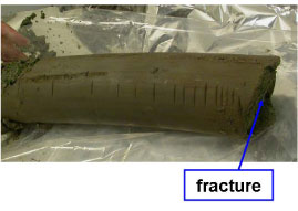
Figure 4.1 - Core sample with fracture location
The detailed concentration profiles as a function of the distance to the fracture are shown for different compounds in Figure 4.2. The distribution of chlorinated solvents is characterized by a diffusion profile with concentration decreasing from the matrix to the fracture (where degradation takes place). In the experiments substrate was injected in the fracture and Figure 4.2 shows a diffusion profile where the concentrations are decreasing with distance from the fracture.
Figure 4.2 - Chlorinated solvents (left) and acids in clay core taken 5 months after injection
These experimental data are used to characterize the diffusive interaction between the fracture and the clay and to determine the key parameters, which control this process.
4.3 Modeling approach
In this section, a simple model is built to simulate the counter diffusion of chlorinated solvents from the matrix into the fracture, where degradation is assumed to take place.
4.3.1 Conceptual model
The aqueous concentration evolution in the matrix after injection of substrate and bacteria is modeled with a 1D-diffusion model.
Figure 4.3 - Conceptual model of counter diffusion out of the matrix into the fracture
Given that each clay matrix block is separated by fractures, then there is a line of symmetry through the middle of each matrix block and the concentration can be modeled between the fracture and the middle of the block. The fracture aperture is assumed to be 2 cm and the clay block is modeled for a distance of 25cm from the fracture. Fast degradation is assumed to take place in the fracture and the concentration is set to zero at this boundary. No degradation is assumed to occur in the matrix, as in this first approach the bacteria (specific degraders) are assumed to be unable to move into the matrix, where pore size may be limited (see Section 4.3.4). The equations in the clay are:
As a result of the symmetry assumption, a zero concentration gradient condition is applied at the boundary of the system (corresponding to the middle of the clay block). Degradation is assumed to occur only in the aqueous phase and not in the sorbed phase, so the model is based on the aqueous concentration. However the measured concentrations are a total concentration, and so it is necessary to convert the aqueous concentration from the model into a total concentration. If sorption isotherms are linear as assumed above, then the total concentration Ctot (dissolved + sorbed amount of compound, µmol.kg-1 bulk) is:
![]()
Where Cw is the aqueous concentration (in µmol/L) and ρb is the bulk density (in kg/L).
A constant initial concentration for DCE and VC is assumed and equal to the measured aqueous concentrations in the fracture before injection of substrate and bacteria. This aqueous concentration should correspond to the total concentration measured in the core sample at approximately 20 cm from the fracture (see Figure 4.2).
4.3.2 Parameters
Field specific data (measured or estimated) are taken from [Jørgensen et al., 2007a] and shown in Table 4.1. To complete the model additional parameters from the literature are needed and these are shown in Table 4.2.
Other parameters can be calculated using the equations shown in the text and are shown in Table 4.3.
Table 4.1 – Measured/assumed parameters for input in model [Jørgensen et al., 2007a]
| Parameters | Symbol | Unit | Value |
| Porosity | φ | - | 0.25 |
| Dry bulk density | ρb | kg/L | 1.99 |
| Wet bulk density | ρtot | kg/L | 2.24 |
| Organic carbon content | foc | - | 0.002 |
| Initial aqueous concentration DCE | Cini,DCE | µmol/L | 32 |
| Initial aqueous concentration VC | Cini,VC | µmol/L | 41 |
Table 4.2 - Parameters from literature for input in model
| Parameters | Symbol | Unit | Value |
| Free diffusion coefficient TCEa | D*TCE | m²/s | 6.23*10-10 |
| Free diffusion coefficient DCEa | D*DCE | m²/s | 7.08*10-10 |
| Free diffusion coefficient VCa | D*VC | m²/s | 8.34*10-10 |
| Octanol-water partition DCEb | log(Kow-DCE) | - | 1.86 |
| Octanol-water partition VCb | log(Kow-VC) | - | 1.38 |
a from [US EPA, 2008]
b from [Abdul et al., 1987]
Table 4.3 – Calculated parameters for input in the model
| Parameters | Symbol | Unit | Value |
| DCE sorption coefficient | KdDCE | L/kg | 0.025 |
| VC sorption coefficient | KdVC | L/kg | 0.008 |
| DCE retardation coefficient | RDCE | - | 1.21 |
| VC retardation coefficient | RVC | - | 1.06 |
| Tortuosity | τ | - | 0.25 |
| Diffusion coefficient DCE | DDCE | m²/s | 1.77*10-10 |
| Diffusion coefficient VC | DVC | m²/s | 2.08*10-10 |
| Initial total concentration DCE | Ctot,ini, DCE | µmol/kg | 4.26 |
| Initial total concentration VC | Ctot,ini, VC | µmol/kg | 4.81 |
From Table 4.3 it can be seen that the initial total concentration in the model is much lower than the concentrations measured on the core sample at a distance > 20cm from the fracture (see Figure 4.2, Ctot,ini,DCE ≈ 35 µmol/kg and Ctot,ini,VC ≈ 18 µmol/kg). As all parameters except for the sorption coefficients have been measured, the difference is due to an underestimation of the sorption coefficients using the empirical Abdul’s equation and the estimated fraction of organic compound (foc). This can be due to the fact that for chlorinated solvents, sorption on clay is not directly proportional to the organic carbon fraction [Allen-King et al., 1996]. In order to match the measured total concentrations, the sorption coefficients must be multiplied by 40, giving KdDCE = 1.04 L/kg and KdVC = 0.32 L/kg.
Experiments conducted at DTU Environment on samples from several field sites (including Rugårdsvej) have given sorption coefficients for cis-DCE and VC around 0.8 and 0.3 L/kg respectively [Zhang, 2008, unpublished]. In these experiments, foc was found to be almost 10 times higher (foc = 0.017) than the estimated value from [Jørgensen et al., 2007a], but this higher value does not explain completely the higher sorption values measured.
These new sorption coefficients are based on core samples analysis and sorption experiments in laboratory. Further research would be needed in this area to determine how the sorption coefficient can be estimated from organic carbon content and if a correction factor should be applied in a general contest.
The retardation factor is a function of the sorption coefficient and a higher retardation factor value results in a slower diffusion of compounds out of the matrix and hence longer remediation times. Based on the newly estimated sorption coefficients, the retardation factor become:
RDCE = 9.4
RVC = 3.6
4.3.3 Model results
The simulated concentration profiles with various Kd-values are shown in Figure 4.4 at a time of 5 months. The new sorption coefficients calculated above allow a better simulation of the profiles. However the simulated profile for DCE does not describe well the measured data from the core samples between 0.05 and 0.10 cm from the fracture. In this simple model it was assumed that no degradation occurs in the clay matrix. DCE reductive dechlorination in the matrix would correspond to VC production, resulting in higher VC concentrations along the diffusion profile, and ethene production through VC dechlorination. But it has been seen in Figure 4.2 that no ethene is present in the matrix.
Figure 4.4 - Simulated diffusion profiles after 5 months for different Kd-values
The difference between the simulated and measured profiles may also be due to an incorrect estimation of one or more parameters. Of all parameters, the tortuosity is the one most probable to have been miss-estimated. Therefore the model was run with different values for t between 0.06 and 0.57 (corresponding to p equal 2 and 0.4 respectively, see Equation ). The slopes of the diffusion profiles decrease with increasing tortuosity factor. A high tortuosity provides a better fit of the DCE concentration profile.
Figure 4.5 - Simulated diffusion profiles for different tortuosity values
The flat part of the measured diffusion profiles for DCE and VC in the first 3 cm next to the fracture could correspond to the presence of a reaction zone. The presence of this reaction zone in the matrix close to the fracture may also be indicated by the detection of specific degraders in this zone [Jørgensen et al., 2007a].
4.3.4 Degradation in the clay matrix
Several scenarios can explain the presence of a reaction zone in the matrix, where reductive dechlorination takes place:
- Presence of micro-fractures perpendicular to the sand fracture, enhancing contact between bacteria, electron donor and chlorinated solvents
- Diffusion and growth of bacteria into the matrix after injection
- Presence of a small population of bacteria in the matrix prior to injection, and growth of this population with the diffusion in the matrix of the substrate injected
The literature relative to this topic is limited and so additional research on the topic is required. Some experimental studies indicate that microorganisms are not expected to migrate or to grow deep within the clay matrix due to the small clay pore sizes, however biomass growth may occur in the clay matrix near the fracture interface [Lima and Sleep, 2007]. Furthermore the presence of this reaction zone at the sand – clay interface does not seem to be directly related to the clay porosity.
4.4 Summary of the matrix sub-model
The transport of the chlorinated solvents in the matrix is characterized by the diffusion coefficient and the retardation factor. Two parameters have been shown to be controlling this process, the sorption coefficient, which may be underestimated with the foc approach, and the tortuosity coefficient. Furthermore the presence of a reaction zone in the matrix close to the fracture is suggested by the results of the model. However the processes responsible for this phenomenon have not been identified.
Version 1.0 July 2009, © Danish Environmental Protection Agency