Model assessment of reductive dechlorination as a remediation technology for contaminant sources in fractured clay: Modeling tool
Appendix G Three different scenarios (advective dominant, diffusive dominant and no fracture)
As explained previously (see Section 2.1 in main report), different conceptual models can describe differences in the geometry of the fracture network. Hence three different numerical models are built to describe each conceptual model, see Figure G.1.
G.1 Scenario presentation
In scenario 1, all contaminant is assumed to flow into the underlying aquifer through the fracture network. Hence the boundary condition at the bottom of the matrix is a zero-flux boundary (outside the fracture). The contaminant flux is then advective and is calculated for one fracture, per unit meter:
![]()
In scenario 2 the contaminant is assumed to flow into the underlying aquifer both by diffusion through the bottom of the matrix and advection through the fracture. Hence the boundary condition at the bottom of the matrix is a specified concentration, corresponding to the underlying aquifer concentration. As it is expected that the aquifer concentration will be very small compared to matrix concentration (dilution), the boundary concentration is set to zero (Cm|z=zbot = 0).
The contaminant flux is then diffusive and advective and is calculated for one matrix block (between two fractures), per unit meter:
In scenario 3, no vertical fractures are present in the clay block and the source zone can be modeled as one homogenous block, where the transport equation for diffusion is applied. All boundaries are defined as zero-flux boundary, except the bottom boundary, where a zero concentration value is assigned. The contaminant flux is then diffusive and is calculated for the entire source zone, per unit meter:
![]()
Where W is the width of the source zone. Note that this is reasonable for large W, otherwise the diffusion is expected to occur in the three dimensions.
Figure G.1 – Illustration of the three transport scenarios
G.2 Assessment of relative importance of advective vs. diffusive flux
The importance of the advective and diffusive fluxes is assessed for different fracture aperture and spacing configurations. Fracture aperture ranges typically between 30 and 30000 µm, while fracture spacing ranges between 0.005 and 1 m [Christiansen and Wood, 2006]. Furthermore fracture porosity ranges between 10-2 and 10—4 [Parker et al., 1997]. Hence, the combinations resulting in porosity out of this range can be disregarded (in yellow in Table G.1) and this results in 16 different configurations of fracture aperture and spacing.
Table G.1 - Fracture porosity for the fracture aperture and spacing configurations
| Fracture porosity | |||||
| 2B in m 2b in µm |
0.005 | 0.05 | 0.1 | 0.5 | 1 |
| 30 | 6*10-3 | 6*10-4 | 6*10-4 | 6*10-5 | 3*10-5 |
| 100 | 2*10-2 | 2*10-3 | 1*10-3 | 2*10-4 | 1*10-4 |
| 300 | 6*10-2 | 6*10-3 | 3*10-3 | 6*10-4 | 3*10-4 |
| 1500 | 3*10-1 | 3*10-2 | 1.5*10-2 | 3*10-3 | 1.5*10-3 |
| 3000 | 6*10-1 | 6*10-2 | 3*10-2 | 6*10-3 | 3*10-3 |
The different simulations are performed with an uniform initial concentration in the matrix and fracture Cm(x,z,t=0) = 100 mmol/m³ and assuming no degradation in the system: the contaminant is removed out of the matrix by the flushing of clean rain water in the fracture.
It can be seen in Figure G.2 that the flux through the bottom of the matrix is not sensitive to variation of fracture aperture. On the contrary, Figure G.3 shows that the diffusive flux increases with reducing fracture spacing, from 9% for 2B = 1 m and up to 23% for 2B = 0.005 m. In these cases the recharge zone of one fracture is reduced (as the fracture spacing is small) and the water flow through the fracture, which is controlling the advective flux, is reduced, resulting in a larger diffusive flux. However the advective flux is the dominant flux in all configurations.
Figure G.2 – Percent of flux through matrix as a function of fracture aperture 2b
Figure G.3 - Percent of flux through matrix as a function of fracture spacing 2B
The influence of applying scenario 1 instead of scenario 2 for the configurations where a diffusive flux of above 10% has been assessed. The main objective of this single fracture model is to evaluate the output contaminant flux from the whole system, whether it comes from diffusion through the matrix or advection along fracture. Hence for a chosen configuration (2b = 10 µm and 2B = 0.05 m), where the diffusive flux represents more than 15% (see Figure G.3) scenario 1 (where there is no diffusion of contaminant through the bottom of the fracture) and scenario 2 are simulated by the numerical model. The outputs of the two models, in term of flux and contaminant distribution in the matrix, are compared. On Figure G.4, the different components (diffusive, advective and total) of the contaminant flux are plotted and it can be seen that the diffusive flux through the matrix represents more than 15% (red line). However comparing the total flux (green line) with the advective flux resulting from scenario 1 (Figure G.5), it can be seen that the two scenarios result in similar contaminant flux at the outlet of the system.
Figure G.4 – Flux at the output of the system in scenario 2 (for 2b = 10-4 m and 2B = 0.05 m)
Figure G.5 – Comparison of total flux out of the system for scenario 1 and 2 (for 2b = 10-4 m and 2B = 0.05 m)
The contaminant distribution in the matrix at different times is shown on Figure G.6. The contaminant distributions are very similar for the two cases, except the presence of a concentration gradient at the bottom of the matrix in scenario 2.
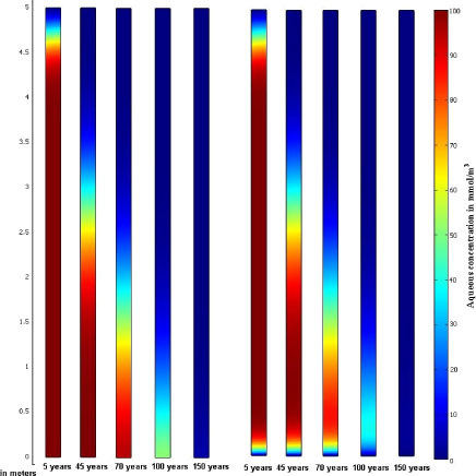
Figure G.6 - Contaminant distribution in the matrix for different times, in case of advection only (left) and (advection and diffusion through bottom of matrix (right)
Disregarding the presence of a diffusive flux through the bottom of the matrix, which can represent between 9 and 25 % of the total flux, does not seem to change the model results, in terms of the total contaminant flux at the outlet and the contaminant distribution in the matrix. Therefore, it was decided to use only scenario 1, for clay systems presenting vertical fractures and scenario 3 for clay system without vertical fractures.
Version 1.0 July 2009, © Danish Environmental Protection Agency