Laboratory Evaluation of Annoyance of Low Frequency Noise
6. Comparison of Subjective Evaluation of Annoyance with Objective Measures
| 6.1 | Danish Method |
| 6.2 | German A-level |
| 6.3 | German Tonal Method |
| 6.4 | Swedish Method |
| 6.5 | Polish Method |
| 6.6 | Dutch Proposal, Sloven |
| 6.7 | C-weighted Level |
| 6.8 | Overview of the Results |
This Chapter describes the assessments made by the reference group and the relation
between these assessments and various objective measures.
In every evaluation the test person was asked to assess the annoyance for two different situations: if the noise was heard in the day and the evening, and if the noise was heard at night. It has been found that there is a very close relation between these two assessments, as is illustrated in Figure 6. Generally the annoyance at night is slightly larger than annoyance in the day / evening.

Figure 6.
Comparison between the assessment made by the reference group of the annoyance in the
day and evening period and the annoyance at night for the same noise examples.
The relation between the pair of evaluations can be described by the correlation coefficient, which is as high as 0.9885. This indicates that it is not necessary to perform a complete analysis on both the assessments, as they are not independent. In the following only the subjective assessment of the annoyance in the night period is considered.
6.1 Danish Method
In this section a thorough description of the analysis process is given. The same analysis method is applied to the other assessment methods, but for the other assessment methods only the results and some comments are given.
In Table 8 below all the noise examples are shown, the names are given in the first column. In the second column the excess of the Danish limit is shown. For the night period the limit value is LpA,LF = 20 dB, but since the drop forge as well as the discotheque are considered as impulsive noises, the limit for these noises is 15 dB. The third column gives the average assessment made by the test persons. Column 2 and 3 are from the presentation with a nominal level of 20 dB, the lowest presentation level. Column 4 and 5 are form the presentations with the middle presentation level, nominally 27.5 dB, and column 6 and 7 are from the loudest presentation with 35 dB nominal level.
Table 8.
Subjective evaluation of the various noise examples shown together with the objective
‘assessment’ by use of the Danish method (LpA,LF).
Nominal level |
20 dB |
27,5 dB |
35 dB |
|||
Noise example |
Excess |
Subjective annoyance |
Excess |
Subjective annoyance |
Excess |
Subjective annoyance |
Traffic noise |
-0,3 |
1,6 |
7,0 |
3,4 |
14,5 |
5,2 |
Drop forge |
6,9 |
4,3 |
14,2 |
5,9 |
21,5 |
6,9 |
Gas motor |
-0,2 |
0,9 |
7,3 |
2,5 |
14,8 |
5,2 |
Fast ferry |
0,1 |
0,9 |
7,5 |
3,2 |
15,0 |
5,4 |
Steel factory |
-1,0 |
1,0 |
5,6 |
2,7 |
13,1 |
4,9 |
Generator |
1,3 |
1,7 |
8,6 |
3,2 |
16,1 |
5,0 |
Cooling compressor |
-0,4 |
2,7 |
6,5 |
4,4 |
14,0 |
6,0 |
Discotheque |
3,7 |
3,0 |
10,7 |
5,4 |
18,1 |
6,7 |
These results are also shown in Figure 7 below. The diamond shaped points are from the
examples with the low level, the square points are from the intermediate level, and the
triangular points are from the highest level.
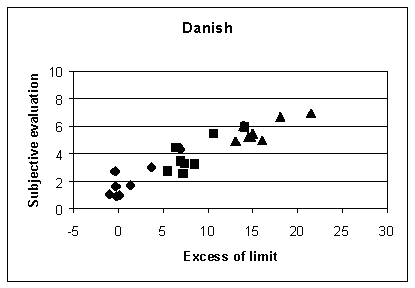
Figure 7.
Illustration of the relation between the Danish assessment method and the subjective
evaluation. Diamonds: low presentation level; squares: intermediate presentation level;
triangles: high presentation level.
The Figure illustrates the subjective evaluation as a function of the excess of the Danish criteria. It is seen that a straight line (not shown in the figure) can represent the group of points. This line is found by linear regression (least squares method, in practise the function LINEST of an Excel spreadsheet is used). The regression line has the formula:
y = 1.61 + 0.26 * x
Where ‘y’ represents the (average) subjective evaluation made by the test subjects and ‘x’ represents the excess of the limit in dB.
The regression line does not explain how well it represents the group of points. Here we can use the residuals, which are the vertical distance between the points and the line. We also use the average of all y-values and the y-values determined by the regression method for each x-value. The determination coefficient or degree of explanation (r2) is defined as:
r2 = SSe / (SSe + SSr)
where SSe is the residual sum of squares, and SSr is the regression sum of squares. In practice r2 is calculated by the Excel function LINEST.
If r2 equals 1.00 there is a perfect linear relationship between the points. If r2 is close to zero, the regression line cannot be used to explain the relation between x and y. In other words, the r2 value indicates how well the points can be described by a straight line. The closer the value is to 1, the better the description.
The relation between x and y can also be described by the correlation coefficient, r . This is calculated as the ratio between the covariance of x- and y-values, and the product of the x-variance and the y-variance:
r = covariance (x,y) / (s x * s y)
The covariance is calculated as the deviation between the x-value and the x-average, multiplied by the deviation between the y-value and the y-average. The x-variance, s x, is the deviation between the x-value and the x-average squared. Similarly the y-variance, s y, is the deviation between the y-value and the y-average squared. The correlation coefficient is calculated by use of the Excel function CORREL. It explains the degree of relation between the x and the y values; it gives a coarse indication of the shape of the swarm of points. If r is close to 1 (or –1) the shape of the group of points has the shape of a ‘cigar’ around the regression line. If r is close to zero, the points lie in a diffuse cloud and there is no obvious relation between x and y.
There is an important difference between the degree of explanation and the correlation coefficient. The degree of explanation, r2, assumes a functional relationship between y and x (e.g. the subjective evaluation is ‘caused by’ the noise). The correlation coefficient does not assume such causality and can be calculated from any two datasets. E.g. in chapter 7 a correlation coefficient is calculated for the annoyance evaluations made by the reference test subject group and the special test subject group. In this situation it is obvious that the ratings made by one of the groups are not caused by the ratings made by the other group.
The values calculated for the Danish method are summarized in the following table.
Slope |
Intersection (x = 0) |
Degree of explanation, r2 |
Correlation coefficient, r |
0.26 |
1.61 |
0.88 |
0.94 |
In the next sessions these statistical calculations are made for each of the different
assessment methods. In every analysis the objective metric is chosen as the x-parameter,
and the subjective annoyance evaluation (which is the same in all cases) is the y-values.
The same scaling is used in all Figures in order to make comparisons easier.
6.2 German A-level
Figure 8 shows the A-weighted level of the noise examples, calculated according to the German standard DIN 45 680. The level is calculated as the sum of the A-weighted levels of those 1/3-octave bands that exceed the hearing threshold. All the noise examples are used in this calculation, including those examples where the noise contains tones.

Figure 8.
Illustration of the relation between the German assessment method using the A-weighted
level and the subjective evaluation
It is seen that the points fall in two groups (two lines); the upper points are the noise examples from drop forge, discotheque, and compressor. The German method (in the present interpretation) obviously cannot give a sufficient assessment of impulsive noise (drop forge and discotheque). The degree of explanation is not too convincing, r2 being 0.54, though r is 0.73.
Slope |
Intersection (x=0) |
Degree of explanation, r2 |
Correlation coefficient, r |
0.19 |
-0.98 |
0.54 |
0.73 |
6.3 German Tonal Method
Figure 9 shows the relation between the subjective evaluation and the tone level above the hearing threshold for those noises that contain tones. The ‘tone/no tone’ decision was made according to the German assessment method. In the figure only one point per noise is shown. This point corresponds to the tone with the greatest excess of the threshold.
The Gas Turbine has two tones above threshold at the highest presentation level (triangle) and one at the intermediate level (square). There is no tone above threshold at the lowest presentation level.
The Generator has one tone above threshold at the highest level (triangle), at the intermediate level (square) and at the lowest level (diamond). The tone is at 80 Hz and thus the level has been reduced by 5 dB according to the German assessment method.
The Cooling Compressor has two tones (50 Hz and 100 Hz) above threshold at the highest presentation level (triangle) and at the intermediate level (squares). As one of the tones is at 100 Hz the level for this tone must be reduced by 10 dB according to the German assessment method. This makes the other tone (at 50 Hz) the greatest. There is only one tone above threshold at the lowest presentation level (diamond).
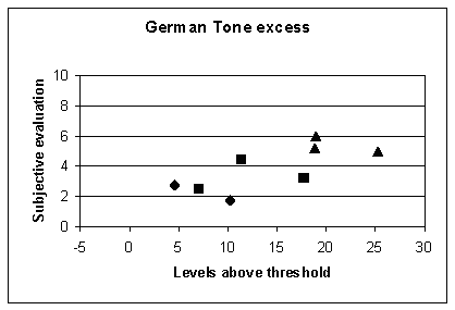
Figure 9.
Illustration of the relation between the German assessment method for tonal noise and
the subjective evaluation
The calculations gave the following results that are very similar to the results obtained from the German A-level method (see section 6.2).
Slope |
Intersection (x=0) |
Degree of explanation, r2 |
Correlation coefficient, r |
0.16 |
1.58 |
0.52 |
0.72 |
6.4 Swedish Method
This method uses a criterion curve that must not be exceeded in any 1/3-octave band. Figure 10 shows the subjective assessment as a function of the greatest excess.
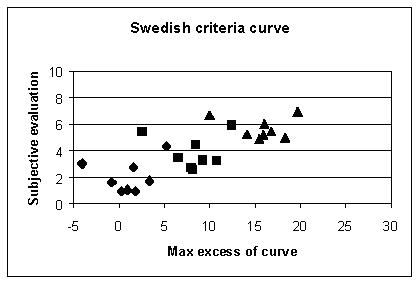
Figure 10.
Illustration of the relation between the Swedish assessment method and the subjective
evaluation
The result of the regression and the correlation analysis is
Slope |
Intersection (x=0) |
Degree of explanation, r2 |
Correlation coefficient, r |
0.22 |
2.10 |
0.57 |
0.76 |
The relation between the subjective assessment and the objective criteria is not too
convincing.
It may be seen from Figure 10 that three points fall ‘to the left’ of the rest of the points. These three points are from the discotheque. Obviously this type of noise should have been assessed about 10 dB ‘higher’ for the points to fit into the rest of the points. The relative low values of r2 and r are mainly caused by these points.
An analysis where the discotheque points have been discarded gave the following result
Slope |
Intersection (x=0) |
Degree of explanation, r2 |
Correlation coefficient, r |
0.25 |
1.34 |
0.81 |
0.90 |
When the discotheque points are removed, the slope of the regression line is almost the
same and consequently the intersection will change. But more importantly it is seen that
the degree of explanation, r2, and the correlation coefficient, r , becomes much greater.
6.5 Polish Method
Figure 11 shows the excess of the Polish criterion curve, which is a curve of 1/3-octave band levels each of which corresponds to an A-weighted level of 10 dB. The other part of the Polish method, which deals with the excess of the background noise level, has not been considered.
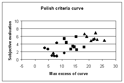
Figure 11.
Illustration of the relation between the Polish assessment method and the subjective
evaluation
It may be seen that the noise examples fall in two rather distinct groups, where (again) the discotheque, the drop forge and the cooling compressor are ‘to the left’ of the remaining points. They should have been assessed at least 5 dB ‘higher’ by the method to align with the remaining points. If one looks at the three groups of points from each nominal level separately (diamonds, squares and triangles), it appears as if the points in each group shows a tendency to a downwards slope to the right; that is, the subjective evaluation decreases as the max excess increases within each group.
The degree of explanation is not convincing, r2 being 0.50.
Slope |
Intersection (x=0) |
Degree of explanation, r2 |
Correlation coefficient, r |
0.20 |
1.00 |
0.50 |
0.71 |
6.6 Dutch Proposal, Sloven
The proposed assessment for use with environmental approval of industries also employs a criterion curve. As is seen in Figure 12 the points spread a lot, and no clear picture can be seen. If one again focuses at the three groups of points from the same nominal level, it appears as if these points slope ‘the wrong way’ as it was seen with the Polish method. As an example (filled squares) it can be seen that when the excess increases from 1 dB to 12 dB, the subjective evaluation decreases from 5.5 to 2.5.
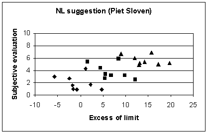
Figure 12.
Illustration of the relation between the Dutch proposed assessment method by Sloven
and the subjective evaluation
Both the degree of explanation and the correlation are rather poor.
Slope |
Intersection (x=0) |
Degree of explanation, r2 |
Correlation coefficient, r |
0.17 |
2.67 |
0.40 |
0.64 |
6.7 C-weighted Level
Figure 13 shows the relation between the C-weighted level of the noise examples and the subjective evaluation. It can be seen that the spread of the points is very large and the correlation is poor. Only the frequency range 10 Hz to 160 Hz is included in the calculation of the C-weighted level.
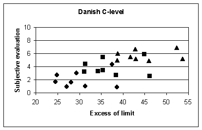
Figure 13.
Illustration of the relation between the C-weighted sound pressure level and the
subjective evaluation
Slope |
Intersection (x=0) |
Degree of explanation, r2 |
Correlation coefficient, r |
0.15 |
-1.82 |
0.44 |
0.66 |
6.8 Overview of the Results
The results of the analysis of the relation between the subjective evaluation and the various objective measures are summarized in table 9 below.
Table 9.
Overview of the results from regression analysis of the relation between the
subjective evaluations made by the reference group and the different assessment methods.
Assess- ment method |
Slope |
Inter- section (x=0) |
Degree of explanation, r2 |
Corre- lation
coefficient, |
Anno- yance |
Anno- yance |
Danish |
0.26 |
1.61 |
0.88 |
0.94 |
-2.3 dB |
1.5 dB |
German A-level |
0.19 |
-0.98 |
0.54 |
0.73 |
10.4 dB |
15.7 dB |
German tonal |
0.16 |
1.58 |
0.52 |
0.72 |
-3.6 dB |
2.6 dB |
Swedish |
0.21 |
2.10 |
0.57 |
0.76 |
-5.2 dB |
-0.5 dB |
Polish |
0.20 |
1.00 |
0.50 |
0.71 |
0.0 dB |
5.0 dB |
Sloven |
0.17 |
2.67 |
0.40 |
0.64 |
-9.8 dB |
-3.9 dB |
C-level |
0.15 |
-1.82 |
0.44 |
0.66 |
18.8 dB |
25.5 dB |
In addition a set of calculations was made on the results of the statistical analysis with
the purpose of comparing the different assessment methods to each other. The rightmost two
columns shows the excess of the criteria from each of the methods that would result from
the same subjective annoyance, respectively annoyance = 1 (on the chosen scale from 0 to
10) and annoyance = 2. These results can be used in a discussion on
‘calibration’ of the assessment methods.
It can be seen from the results that the assessment method with far the best correlation between the subjective and the objective assessment is the Danish method, using the A-weighted level in the frequency range from 10 Hz to 160 Hz. The degree of explanation is high, and there is no obvious indication in the results obtained here of ways to further improve the method. The second best method is either the Swedish method, based on a criterion curve, or the German method using the A-weighted level.
It is seen from the rightmost column that a noise that would exceed the Danish criterion by 1.5 dB will give rise to a subjective annoyance of 2 (on a scale from 0 to 10). The same noise would be 0.5 dB below the Swedish criterion and would give rise to a German A-weighted level as low as 15.7 dB. Thus it can be stated in broad terms, that when the assessment methods are compared in this way with representative noise examples and ‘calibrated’ to the same subjective annoyance
| the Swedish method is a little less restrictive than the Danish method (that is, the Danish limit value - for the evening and night period - corresponds to a lower annoyance than the Swedish method) | |
| the German method for broadband noise - using a limit value of 25 dB for the night period - is considerably less restrictive than the Danish method. On the other hand, the German method for tonal noise is a little more strict than the Danish method. Thus the German method change significantly with the appearance of tones in the noise | |
| the Polish method appears more restrictive than the Danish method, though in this comparison the ‘release’ of the Polish criterion at higher frequencies that results from considering the background noise has not been implemented, and | |
| the Dutch method proposed by Sloven is somewhat less restrictive than the Danish method. |
These results cannot be used to decide which of the methods that are unnecessarily strict or too relaxed, since the results are based on a limited number of noise examples only.