Scenarios and Model Describing Fate and Transport of Pesticides in Surface Water for Danish Conditions
Appendix D
1 Uncertainty Analysis of the Registration Model
1.1 General statements about different sources of uncertainty
When models are applied in decision-making processes an evaluation of the uncertainty of the model predictions is crucial. Some kind of uncertainty estimate is needed before the model system can be said to have any predictive power because it is not possible to evaluate a calculated property if no information about the uncertainty exists. However, it is difficult and in praxis even impossible to perform complete uncertainty estimates that take all sources of model uncertainty into account. However, this does not mean that the model uncertainty cannot be evaluated. The task is to gather as much information as possible about the model uncertainty before the model system is applied.
There exist two principally different sources of uncertainty relating to the predictive model itself:
- Structural uncertainty arising form the assumptions needed for the model equations to describe the phenomenon in question.
- Input parameter uncertainty as a consequence of variability and lack of knowledge
Often there will be a trade off between these two sources of uncertainty. Increased model complexity can take more complex mechanisms into account in the model and thereby reduce the structural uncertainty. This will consequently increase the numbers of needed input parameters and thus the tendency for the input uncertainty to influence the final result. This may not be a problem if there are sufficient resources to establish sufficient quality input parameters. If the latter is not the case, then the input uncertainty can easily increase considerably. So the reduced structural uncertainty gained by increasing the model complexity can easily be overruled by increased input uncertainty ending up with an increased total uncertainty. The optimal complexity level for a model to be used in a specific case will thus depend on the available resources for collecting input parameter values.
Methodologies for performing structural and input parameter uncertainty estimates are different. The structural uncertainty can only be truly estimated in cases where the total uncertainty on input parameters is known and the model predictions can be compared with “reality” at the same time. This introduces the need for high quality data to validate the model. This approach will not be a part of this specific this work. It is however important to emphasise that if sufficient data are available to make a complete determination of the structural uncertainty, then data are needed for all possible model outcomes and in these cases there is no need for predictive models for decision making. Contrary, there exist straightforward methods for quantifying the input uncertainty typical by using a MonteCarlo type analysis. But, they often involve laborious calculations for larger models like this registration model. So the topic for this part of the work is to set up guidelines in order to make it possible to perform uncertainty analysis using the registration model and a Monte Carlo type procedure.
The submodel system has common input parameters, e.g. Kd and kdeg as well as separate parameters, e.g. dispersion coefficients, and some input parameters are even derived in other submodels, e.g. pesticide concentrations found in groundwater act as input to the stream model. In contrast to the quantification of the structural uncertainty, the quantification of the input uncertainty is rather straightforward based on a series of different methods. However, it is important to emphasise that analysis of input uncertainty needs to be done carefully in order not to create false realism. Uncertainty analysis for predictive models is often by itself rather uncertain, where the uncertainty estimates are associated with uncertainty. The uncertainty on input parameters can be estimated by evaluating the following two topics
- Uncertainty due to the assumed functional form of the stochastic relationship for input parameter variability.
- Missing information due to the limited number of single data values to estimate the variability of the input parameters.
The type A uncertainty can e.g. be a result of an assumed log-normal or equal distribution of input data. When the distribution function for the input data is assumed known then the type B uncertainty arises from the fact that the distribution-function parameters (e.g. mean value and variance) needs to be estimated based on a limited number of data values.
The analysis is therefore based on a tiered approach, where more and more complex sub-models are analysed for input uncertainty towards the final complexity level of the model system. In this way it will possible to perform the large amount of calculations needed to map the nature of the uncertainty. The principle of the sub-models is that they shall reproduce the process and transport mechanism in the complete model but under more simple spatial and temporal conditions.
1.2 Principles of the uncertainty analysis
The purpose is to assess the uncertainty of the calculated pesticide concentrations in the stream and pond compartments as a function of the uncertainties on input parameters. For this purpose a Monte Carlo analysis will be performed as illustrated in Figure 1.1. The model will be run a predefined number of times, and each time the input parameters will be changed according to the distribution function. The variability of the modelling result reflects the uncertainty due to input parameters. This is illustrated in Figure 1.1. If all possible input parameters in a large model are going to be investigated using this type of analysis then often an unrealistic large number of model runs are needed. So, a critical aspect is to identify a limited number of input parameters in the uncertainty analysis that account for major part of the uncertainty.
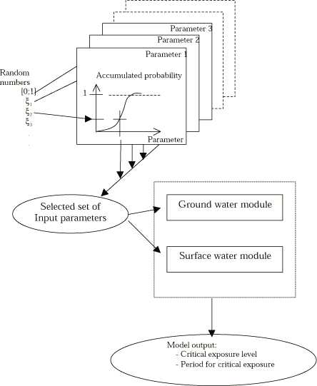
Figure 1.1 Principles for uncertainty analysis based on Monte Carlo simulations. input parameters are assumed being normal or log-normal distributed. Output parameters from the soil model (drain) are linked to the boundary conditions for the ground water, stream and pond submodels. The endpoint is uncertainty estimates on critical stream output parameters.
1.3 Process description and uncertainty on physico-chemical input parameters of special concern
Within this project are included experimental investigations of the sorption-desorption properties as well as degradation of the three pesticides, Dipendimethalin, Bentazon and Ioxynil. However, the Pesticide And The Environment data base, PATE, which is the Danish EPAs database on pesticides is expected to be the input parameter data source used in the registration model. The database, as any database, includes data derived from different laboratories, using different analytical as well as modelling approaches. It is a challenge to identify the true variability of the parameters in relation to the purpose of modelling. The use of a Freundlich type adsorption for equilibrium adsorption in the soil system and the diffusion coefficient used in the pond model are both areas where special attention is needed which will be analysed in the next two paragraphs.
1.3.1 Problems related to the use of Freundlich type adsorption
One important pitfall has been identified for the modelling of adsorption using a Freundlich adsorption description. As this way of modelling adsorption plays a central role in the assessment of pesticides there is a need for discussing the modelling paradigm as well as the structural uncertainty introduced by using this equation at low concentrations. Sorption experiments are usually undertaken using relatively high concentration levels in the magnitude of 1 µg/ml (1 mg/l), which is about 1000 times higher than the actual concentration levels of possible concern in the environment. These experimental results are used to extrapolate to lower concentration levels that are realistic in the environment. This is not a problem if linear or Langmuir type of adsorption is used, but it can be very critical when a Freundlich adsorption is applied. This will be documented in the following ending up in an illustration using experimental data on Bentazon.
Natural media are multi-component systems consisting of several phases and solutes. Such systems could be solutes partitioning between an aqueous bulk phase and soil particle or e.g. suspended organic matter. The molar fraction of the individual pollutants, xi, is small with respect to the molar fraction of the bulk water, xw, in natural environmental aqueous compartments. In such systems any organic pollutant will be the minor component, i.e. xw>>xi. Therefore, with respect to the pollutant contamination, most aqueous compartments are properly described as dilute solutions. Experimental measurements performed in the laboratory can be described as a system consisting of a single solute partitioning between two immiscible (organic matter and water) phases, which constitutes a closed system, i.e. heat and work are exchanged with the surrounding, but the solute never leaves the two-phase system. The two phases, within the closed system, are open systems and the solute can be transferred from a polar phase, I, to a non-polar phase, II.
If we assume that the conditions for the partitioning solute in every phase is a dilute solution state, then the chemical potential of the solute is given by
![]() (1.1)
(1.1)
where Ci is the molar concentration of the solute in a given phase, the standard chemical potential being defined at the infinite dilute solution state (Thomsen, 2001). At equilibrium the chemical potential of the solute are equal in each phase and the equilibrium partitioning an be derived as follows
![]() (1.2)
(1.2)
where µio,I and µio,II are the standard potential for respectively phase I and II. By assuming ideal dilute solution state in both phases, the activity coefficient γi is unity and the equilibrium partitioning of the solute from the polar phase the non-polar phase. Ideal solution is in general a good approximation for very dilute solutions.
![]() (1.3)
(1.3)
In the case of the polar phase, I, being water, and the non-polar phase, II, organic matter Equation App5.3 can be expressed as
![]() (1.4)
(1.4)
This is how the equilibrium partitioning coefficient is defined for ideal dilute two-phase systems for which Kd can be quantified as the molar concentration ratio of component i in two slightly miscible or immiscible phases. The quantity Δµi0 is a constant for γi constant (very dilute conditions) so the equilibrium adsorption coefficient Kd will approach a constant when the water concentration approaches zero.
Freundlich isotherm
The Freundlich sorption isotherm tries to describe the non-ideal situation, i.e. where the equilibrium-partitioning constant depends on the concentration of solute in the experimental system, through the empirical equation
![]() (1.5)
(1.5)
where Cis is the concentration of the compound i in the suspended or solid non-aqueous phase, Ciaq is the concentration of pollutant dissolved in the aqueous bulk phase, KF is the Freundlich constant and n a factor defining the shape of Cis a function of Ciaq. Using the Freundlich description it is possible to calculated the resulting Kd value as a function of the water concentration as
![]() (1.6)
(1.6)
For n<1 this equation predicts the Kd value to approach when the water concentration approach zero, while for n>1 the Kd value will approach zero for low water concentration values. Both cases of either n<1 and n>1 are in conflicts with the thermodynamic lined out above having constant Kd for small concentration levels. Only in case of n=1, where the Freundlich approach reproduces the linear adsorption description ia there a coincidence with the thermodynamic theory. This is a very critical issue for the uncertainty analysis when the concentration level used in an adsorption test is higher than the concentration level simulated by a model which have used the results from the adsorption test. The Freundlich description becomes more and more in conflict with the theory of adsorption for decreasing concentration levels ending up in infinite high uncertainty for infinite low water concentration. So the structural uncertainty is a seriously problem when experimental data fitting of higher concentration levels using Freundlich are used for lower concentration modelling. Another problem in relation to the use of Freundlich for lower concentration values is that the importance of the input uncertainty increases dramatically as the concentration decreases. This is easy illustrated using Equation 1.6 and assuming a “error” of Δn on exponent n. It is then possible to express two alternative Kd values as
![]() (1.7)
(1.7)
The ratio between these two alternative Kd values is
![]() (1.8)
(1.8)
As the cw value approach zero this ratio will approach infinite telling that all Kd values are possible! This will be illustrated later using Bentazon and data from the PATE database.
Despite the nonsense lower limit condition of the Freundlich equation, non-linear partitioning between an aqueous and a non-aqueous phase with n<1 is observed for many hydrophobic and specific interacting chemicals, e.g. like the pesticides. In this respect, the Freundlich isotherm is nice as is fits all experimental data. However there are several additional aspects that makes it questionable / unreliable to use the Freundlich isotherm, which are e.g.:
- most often the concentration in the solid or non-aqueous phase is calculated from the measured concentration of solute in the aqueous phase.
- the equilibrium partitioning coefficient depend on the activity in each phase and can not be quantified through the concentration of solute in each phase (Equation 1.4)
- Hydrophobic and specific interacting chemicals have tendencies to sorb to interfaces, and they form dispersions or emulsions within the aqueous phase upon reaching saturation of the aqueous bulk phase. The latter may occur locally due to inappropriate sample preparation methodologies and slow kinetics in three-phase systems, which may explain why desorption experiments often result in significantly larger equilibrium partitioning coefficients than sorption experiments.
- Most analytical techniques do not have the capability to discriminate between true solutions and solutions including a dispersed phase, which may be the explanation why partitioning values are often underestimated, and furthermore increasingly underestimated by increasing hydrophobicity of the test chemical.
- Sorption to the inner walls of the test tubes have shown to increase by mechanical shaking, while desorption phenomena occur upon silence.
- Equilibrium partitioning experiments are often based on the shake-flask method
- The concentrations of chemicals within the natural environmental are most often much lower that experimental concentration levels.
- The Freundlich isotherm is fitted based on very few measurements at the high concentration region by extrapolating into the low concentration area. A worst case scenario is that the size of n depend on the developing stage of a third dispersed phase, and thereby the degree of underestimation of KD as a function of the concentration of test chemical in the measured system.
So, there are many experimental pitfalls, which may very well explain the observed non-linearity in equilibrium partitioning values.
It is not unrealistic that experimental aqueous concentrations of the test chemical are 1000 times larger that the actual concentration occurring the aqueous phases of the natural environment. This means that we would have to estimate the equilibrium partitioning concentration in the low concentration based on extrapolating from higher concentrations. Such a data set is shown for Bentazon in the Figure 1.2 below.
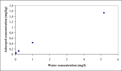
Figure 1.2 Experimental data on measured concentration of Bentazon in the solid phase versus the bulk water phase.
In Figure 1.2 the concentration levels are high (the unit on the x-axis is in the mg range). At first it seems that this is not a problem due to the large difference between the smallest and largest test concentration. Four different adsorption tests are undertaken for Bentazon and the following Freundlich coefficients are determined:
Table 1.1 Freundlich coefficients based on data from four individual adsorption experiments
| Experiment no. | KF | n |
| 1 | 0,45 | 0,688 |
| 2 | 0,38 | 0,696 |
| 3 | 0,42 | 0,664 |
| 4 | 0,18 | 0,561 |
The variability of the coefficients is limited for these tests, so the uncertainty related to the adsorption coefficients seems relatively small. This uncertainty can be quantified for fixed water concentration by calculating Kd using the KF values and Equation 1.5 in a Monte Carlo simulation, where the variability of the coefficients in Table 1.1 are included. Monte Carlo simulation, based on data given in Table 1.1, for different levels of fixed water concentrations, cw, have been used for estimating the probability density function for Kd which is shown in Figure 1.3 below.
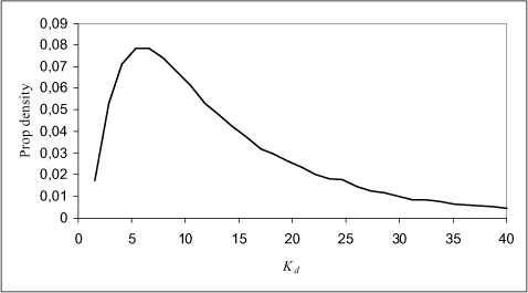
Figure 1.3 The probability density function is calculated at Cw=0.01 µg/L and varying Freundlich constant, KF, and n according to experimental data from four studies extracted from the PATE database (PATE, 2001).
The uncertainty in Kd is increasing drastically at small concentrations in the aqueous phase, which is illustrated in Figure 1.3 as predicted by Equation 1.5. In Figure 1.4 below the logaritmic transformed Freundlich isotherm is compared to a simple linear regression fitting the dilute solution description (Equation 1.4).
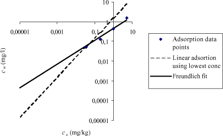
Figure 1.4 The figure illustrates logcw as function of logcs, the blue dots representing experimental data. The solid line represents cw as function of cs calculated based on the Freundlich parameters KF and n, the dotted line represents cs calculated based on Kd value calculated using the lowest concentration values in the test.
As seen from Figure 1.4 the Freundlich equation fits the experimental data quite well. However, Kd is increasingly overestimated at decreasing concentration of solute in the aqueous phase. At environmental realistic concentration, the equilibrium partitioning value may be up to 700 times larger than the Kd value based on n=1. The most reliable method of extrapolation is to use the data originating from the lowest aqueous measured concentrations letting the intercept equal zero and this value is shown as a dotted line in Figure 1.4.
1.3.2 The effective diffusion coefficient
The importance of the sediment uptake both in relation to degradation and accumulation of substance is very much controlled by the diffusion coefficient. In conventional risk assessment the diffusion coefficient is estimated based on molecular diffusion experiments or based on calculations of molecular diffusion for other substances. When this is performed it is very important to evaluate the assumption of one-dimensional diffusion in the model for risk assessment. The one-dimensional model for diffusion will in principle become invalid at a sufficiently small length scale. Detritus and growth of algae yielding a high surface area for diffusion will cover the bottom of the pond. Thus, if the diffusion takes place only in the surface the area for diffusion may be very much larger than the simple gross section area. If the effective area for diffusion is larger than the cross section area in the model then the diffusion may be heavily under estimated and a “hidden” uncertainty will be a reality (Mogensen et al., 2004). Below a length scale is derived and guidelines are set up to deal with the problem.
For constant dissolved water column concentration and no degradation in the sediment the concentration profile is given as (Mogensen et al., 2004)
![]() (1.9)
(1.9)
where erfc is the complementary error function. The depth for diffusion can be defined in different ways. In this investigation it is important to find a depth where most of the substance will be in the sediment above. The depth where sw is only 10%of cw,o is defined to be the diffusion depth (x0,1) in this investigation yielding the following relationship
![]() (1.10)
(1.10)
where Equation 1.9 is used in the derivation. D will be approximately constant for non-polar organic substances and a value around 5·10-10 m²/s is a realistic estimate (Mogensen et al., 2004). However, the retardation factor R can be highly variable between different substances.
Below the length scale of the diffusion depth will be calculated for pendimethalin using a R value of 1300 as presented above. The depth seems very small even after several days of diffusion. The diffusion can clearly not be assumed one-dimensional when the major part of the substance mass in the sediment is in a depth lesser than a mm.
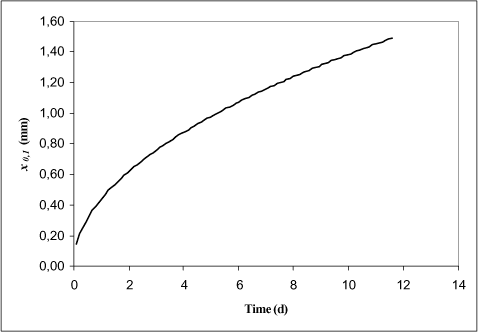
Figure 1.5 The Diffusion depth in mm for pendimethalin as a function of time (days).
One way of handling this problem is to use an “effective” diffusion coefficient, which is much larger in value compared to the molecular diffusion coefficient. It is not possible to compensate completely for the effect of the large surface area, but as a pragmatic solution the diffusion coefficient should be increased for highly adsorption substances like pendimethalin.
1.3.3 Uncertainty in relation to the Henrys Law Constant
The Flux due to evaporation will be assumed to follow the equation as
 (1.11)
The coefficient Kw is given by
![]() (1.12)
(1.12)
where kg is given as
![]() (1.13)
(1.13)
The aerodynamic resistance (ra) is assumed negligible in the following derivations and the resistance term rb is described as
![]() (1.14)
(1.14)
where κ=0.4, µ*=0.3 m/s, ![]() (zom=0.01 m) and the Smith number (Sc) is related to the diffusion coefficient in the air as
(zom=0.01 m) and the Smith number (Sc) is related to the diffusion coefficient in the air as
![]() (1.15)
(1.15)
where ν is the kinematic viscosity and can be estimated to be 1.55+10-5 m²/s.
The Dg value can be calculated from:
![]() (1.16)
(1.16)
Equations 1.13 to 1.16 yield
![]() (1.17)
(1.17)
Equation 1.17 shows that kg is nearly independent on the properties of the substances because of the relatively low power of the exponent for MB. The variability of kgdue to different substances can be estimated using a typical molar weight interval from 200 g/mol to 400 g/mol as kg = 0.021 down to 0.017 or a change of 18%, which is a rather limited deviation taken all other uncertainties into account.
The transfer coefficient (kw) is described as
![]() (1.18)
(1.18)
In the following the influence from derivation in temperature will be neglected (Θ≈1). The K2d is given as
![]() (1.19)
(1.19)
The water velocity can be calculated for “friction dominant flow”, which is a good approximation for smaller streams, using the Manning formula:
![]() (1.20)
(1.20)
where Q (m³/s ) is the flow and w (m) is the width of the stream. The diffusion coefficient in water (Dw) is given as
![]() (1.21)
(1.21)
Combining Equations App5.18 to App5.21 yields
![]() (1.22)
(1.22)
Equation 1.22 shows that the value of the mass transfer coefficient, kw, is mostly influenced by the actual value of I. Secondary, kw is influenced by the ratio between the water flow, Q, and the width of the stream, w. The Friction coefficient in the stream, M, will hardly have any influence in the gas exchange due to the low power value of 0.054. In the same manner it is possible to exclude the molecular mass as important, where a change in molecular mass from 100 g/mol to 500 g/mol will introduce a change in the MB0.295 value from 3.9 to 6.3. In case of a smaller stream, then following hydraulic parameters values can be used: I=0.005, M=30, Q=0,01 m³/s, w=1 m, which ends up in a value as kw=2.4·10-5 m/s.
The influence of H can be quantified using Equation 1.12. If H is “large” then Equation 1.12 predicts Kw as equivalent to kw and in this case the uncertainty on H will not be important for the release of substance to the air as this will only be covered by water phase transport processes nearly independent on substance specific conditions. On the other hand if the H values is small then the evaporation from the surface will become limited and thus the uncertainty on the actual H value unimportant. The following relationship is defined in order to identify the critical interval of H in which the uncertainty will be most important.
A change in the Kw value due to a change in the H value can be estimated for “small” changes using a first order uncertainty analysis. This is not very useful for predictions when the variation on physico-chemical parameter values are large as often seen in exposure models. However, in the following the first order analysis is used to map the sensitivity and thus identify where in the parameter space the uncertainty will tend to be most important. Subsequently a Monte Carlo analysis can identify the actual related uncertainty level.
The following first order uncertainty equation is used:
![]() (1.23)
(1.23)
where the Δ denotes the interval, so ΔKw is the interval of Kw formed as a result of the interval of H as ΔH. The relative uncertainty on H is more relevant to investigate compared to the absolute uncertainty so the relative interval of H is defined as ![]() and using this defined combined with Equations 1.12 and 1.23 yields
and using this defined combined with Equations 1.12 and 1.23 yields
![]() (1.24)
(1.24)
The special case where the only removal is evaporation can be described using a simple first order removal equation as
![]() (1.25)
(1.25)
The most significant change in concentration level will be in the down stream outlet from the stream having the length L and the time period for the removal to take place will then be ![]() . It is now possible to estimate the interval of
. It is now possible to estimate the interval of ![]() as a function of the actual relative interval of H for a given H value using
as a function of the actual relative interval of H for a given H value using ![]() as
as
![]() (1.26)
(1.26)
This relationship is used to analysis the sensitivity for different H values in the following figure, where the length L is equal 3000 m and the hydraulically properties equal to the values lined out above.
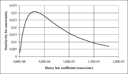
Figure 1.6 The sensitivity of the model output to the variation of the input data for Henrys Constant as a function of the size of Henrys Constant
1.4 Stream model
1.4.1 Hydraulic model
The simplified stream model is based on a series of assumptions
- Steady state hydraulics.
- Geometry is uniform in the direction of flow.
- Cross section is rectangular.
- Flow into the stream consists of an initial inflow upstream (from large drain systems) and a linear inflow (drain and/or ground water) in the direction of flow toward the outlet to the shore.
- The flow is friction dominant using the so-called Manning equation.
- The water depth in the stream is calculated based on steady state hydraulics.
Figure 1.7 Longitudinal section showing the hydraulic relationships of the stream.
A rectangular cross-section is assumed as shown in Figure 1.8.
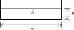
Figure 1.8 Cross section of stream model.
Strong turbulence is assumed and thus the Manning equation is
![]() (1.27)
(1.27)
where A is the cross section area, M is the friction (Manning) number, I is the water surface slope and as illustrated in the equation the bottom slope (Io) will be used as approximation for I. R is the hydraulic radius and for the rectangular cross section it is given as:
![]() (1.28)
(1.28)
The depth is assumed “small” compared to the width (w). In hydraulic steady state conditions the Equation 1.27 can be used to calculate h using Equation 1.53 as
![]() (1.29)
(1.29)
1.4.2 Quasi steady-state stream model
In this paragraph steady state equations will be derived which can determinate the steady state concentration values in the different compartment of the stream. In steady state the adsorbed concentration levels in relation to fixed compartments such as sediment solids and macrophytes (sw and cm) are in simple equilibrium with respectively the dissolved concentration values in sediment and water column. On the other hand the dissolved concentration levels (cd and sw) and the adsorption to moving solids in the water column (cs) will most likely be in dynamic equilibrium and thus determined by the transfer and process mechanisms. In the following equations are derived to calculate the cw, sw and cs values.
The following fluxes of matter take place in the stream model:
Figure 1.9 Steady state box-model of the stream.
Transport and process related fluxes taken as positive in relation to Box n:
Convective transport in:
![]() (1.30)
(1.30)
Convective transport out:
![]() (1.31)
(1.31)
Dispersive transport:
 (1.32)
 (1.33)
Lateral transport:
![]() (1.34)
(1.34)
Exchange with the atmosphere:
![]() (1.35)
(1.35)
Exchange with the sediment:
![]() (1.36)
(1.36)
Exchange between dissolved and suspended fraction in water column, where increasing cw is taken as positive:
![]() (1.37)
(1.37)
Degradation in water column:
![]() (1.38)
(1.38)
Degradation in sediment:
![]() (1.39)
(1.39)
Exchange with macrophytes:
![]() (1.40)
(1.40)
Degradation on macrophyte surface
![]() (1.41)
(1.41)
Eliminating sw,n
At steady state the degradation in the sediment will be equal to the flux from water column to sediment as:
![]() (1.42)
(1.42)
Eliminating cm,n
At steady state the degradation on the macrophyte surfaces will be equal to the net adsorption rate to the macrophyts thus
![]() (1.43)
(1.43)
Isolating cw,n
Mass balance at steady state, yielding equal sum of fluxes:
![]() (1.44)
(1.44)
Using the equation for the flux values and Equation 1.44, the following relationship is derived:
Click here to see Equation 1.45
The nominator of Equation 1.45 is independent on the concentration values, but depends on the position (n). It is therefore convenient to define a coefficient (z1n) as
Click here to see Equation 1.46
Equation 1.71 can be rewritten as
![]() (1.47)
(1.47)
where
 (1.48A)
![]() (1.48B)
(1.48B)
![]() (1.48C)
(1.48C)
![]() (1.48D)
(1.48D)
Isolating cs,n
The following fluxes are relevant for the steady state mass balance of the suspended concentration cs,n:
![]() (1.49)
(1.49)
The resulting equation can now be derived:
 (1.50)
which can be rewritten as
![]() (1.51)
(1.51)
where
![]() (1.52A)
(1.52A)
![]() (1.52B)
(1.52B)
![]() (1.52C)
(1.52C)
![]() (1.52D)
(1.52D)
It is important to notice that the derived equation for the concentration level at a given position is linear related to the concentration level in the neighbour positions. Thus the concentration levels in the stream will respond linear in relation to the concentration level in the in flowing water from drain and ground water. So, the relative uncertainty in the in flowing concentration level from the soil model will tend to induce the same magnitude in the stream modelling results.
1.4.3 Non steady-state stream model
Dissolved substance:
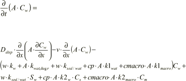 (1.53)
where the mean cross-section water velocity (v) is given as
![]() (1.54)
(1.54)
Adsorbed to suspended particles:
![]() (1.55)
(1.55)
Adsorbed to the macrophytes:
![]() (1.56)
(1.56)
Pore water concentration in the sediment:
![]() (1.57)
(1.57)
The concentration adsorbed to sediment solids:
![]() (1.58)
(1.58)
The mass adsorption/desorption parameters (k1 and k2) is related to the solids concentration as
![]() (1.59)
(1.59)
where Cp is the solids concentration and k1'and k2' are rate constants per amount solids
The differential equations are solved using a finite difference technique.
1.4.4 Uncertainty analysis of parameter influence in stream model
Model sensitivity towards variations in process parameters is investigated through the following scenarios
1) Non steady-state (dynamic) model.
2) Quasi steady-state model.
Parameter variability can be attributed to
- Variation between pesticides. All pesticides included in the PATE database are considered, and mean parameter values are used for each pesticide.
- Stochastic variability of parameter values for individual pesticides. MonteCarlo analysis is performed for the hydrophilic pesticide bentazon, and the hydrophobic pendimethalin. The values in Table 1.2 are used.
Table 1.2 Parameters for bentazon (hydrophilic), pendimethalin (hydrophobic) and aggregated values for all included pesticides. The values are assumed log-normal distributed and are obtained from the PATE database (PATE, 2001) and from DHI?.
| Parameter | Bentazon | Pendimethalin |
| logKd | -0.4288 ± 0.2550 | 1.7593 ± 0.0194 |
| logkdeg | -6.4976 ± 0.3121 | -6.5751 ± 0.2048 |
| logKdmacro | 1.09 ± 0.78 | 0.65 ± 0.0001 (= 0) |
Values for the sorption equilibrium coefficient and aerobic degradation rates are available for 37 pesticides, whereas the macrophyte sorption equilibrium coefficient is only available for 11, including bentazon and pendimethalin. Henrys Law constant is given for pendimethalin only.
logKdmacro = 1.15 ± 6.56 (11 pesticides)
logKH = -0.372347 ± 0,135242143 (1 pesticide)
In case a) the mean values for Kdmacro and KH are used for all pesticides. In case b) the Kdmacro and KH values in Table 1.2 are used, except for bentazon where the mean logKH is used.
The 1st order adsorption constant is logksorp = -3,262031231 (2 pesticides). It has been empirically determined based on measurements on sorption kinetics in ref. Christian?. The 1st order desorption constant is kdesorp = kdesorp/Kd.
On the basis of measurements on suspended organic matter and macrophytes for the Odder Bæk and Lillebæk systems, estimated mean concentrations and standard deviations for assumed log-normal distributed data are
| Organic matter: | logCP = 1.114737 ± 0.416499 |
| Macrophytes: | logCmacro = -0.67474 ± 1.043952 |
1.4.4.1 Non steady-state
A simple way to investigate the influence of parameter variations is by considering a steady-state situation. However, it is necessary to find the time interval for steady-state to occur and to investigate whether
extreme situations occur prior to steady–state conditions.
In the figure below the development in concentration in bulk water, sediment and on macrophytes is shown for bentazon. The inlet bulk water concentration, Cw, and concentration of pesticide sorbed to suspended particulate matter, Cs, are set to one. This corresponds to a situation where substance is introduced continuously to the stream through drain at x = 0.
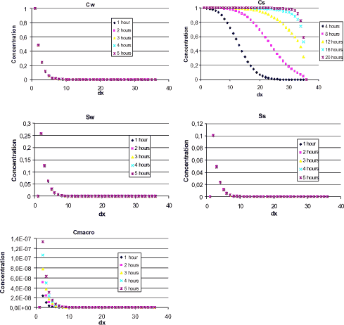
Figure 1.10 Output from Non steady state stream model. concentration in bulk water,CW, suspended particles,CS, sediment pore water, SW, sediment particles, SS and macrophytes, Cmacro, respectively are shown. Mean values of logKd, logksorp, logkdesorp, logkdega, logkdegan, logKH, logKdmacro and logKsedwat = -3.0 has been used. Calculations are made for up to five hours, except for Cs, which is calculated up to 20 hours.
Concentrations are calculated with one-hour intervals and stops at five hours, except for Cs, which continues up to 20 hours. Steady-state is achieved for all concentrations, except Cs, within five hours. Bentazon is relatively hydrophilic and the sorption rate is therefore low, in other words the time for reaching the maximum sorption capacity (in steady-state) is long.
The bulk water concentration, Cw, decreases as a consequence of sorption, degradation and exchange with sediment pore water and “clean” water at 3500 m. For most substances kdeg and kdesorp are considerably lower than ksorp, which implies that the particles that are transported in the bulk water down the stream with the initial concentration Cs of 1, maintain this concentration throughout the longitudinal axis. For bentazon with Kd below 1, it takes some time before sorption equilibrium occurs between the mobile particulate matter and the bulk water. No deposition takes place (ksedwat reflects only bulk transport between stream water and sediment pore water), therefore no loss in sorbed concentration is seen in the bulk water down stream at steady-state, and no increase is seen in the sediment particles Ss. In fact Cs increases slightly down the stream due to sorption of substance from the bulk water. At a certain point the desorption from suspended particles levels out sorption from the bulk water, due to low Cw. This is most clearly seen for hydrophilic substances.
The sediment particles are stationary contrary to bulk water particles, which move down the stream. The sediment particle concentration, Ss, follows the sediment bulk concentration levels, Sw, through sorption, which again follows stream bulk water, Cw, through water exchange, ksedwat. Again, sorption is often much faster than desorption and degradation and the sediment particle concentration is accordingly high due to sorption from the bulk (sediment and stream). The qualitative macrophyte concentration profile, Cmacro, resembles the sediment concentration, as the macrophytes are also stationary. They are however more closely linked to the stream bulk water concentration, Cw. The concentration in particulate matter is pr. total volume; i.e. Ss is larger than Cmacro, due to higher density of particles in sediment than of macrophytes in bulk water.
The dynamic behaviour of substances depends on the physico-chemical process rates and on the hydraulic conditions of the stream. The hydraulic retention time in the bulk water, cf. Equation 1.60, is tret = 0.37 hours. The half-life for bentazon is approximately 800 hours and the sorption time to suspended matter in the bulk water is approximately 40000 hours, calculated as (ksorp ρparticulate matter)-1. The sorption time to macrophytes is even longer due to the lower mass per total volume ration of macrophytes.
For hydrophilic substances such as bentazon, the time for reaching steady-state is within a few hours, with the exception of Cs, where it occurs after about 20 hours. When the pesticide fate in the environment is considered, tidal intervals must be considered in relation to the slowest processes. With respect to pesticide application on crop and soil the time periods for drain flow through soil is in the scale of hundred days, even for hydrophilic pesticides. Concentrations in stream bulk water, sediment and macrophytes can therefore be considered to be in steady-state.
1.4.4.2 Quasi steady-state
It has been shown that an analysis of the dynamic behaviour of the stream model is redundant when the stream receives substance from leaching through soil. The uncertainty analysis can therefore be
performed with the quasi (because it changes with drain inlet) steady-state stream model.
The calculations are made after a time period of 10 hours, which is an adequate time interval for a steady-state situation to be established in the stream, when the border conditions are kept constant. The inlet bulk water concentration, Cw, and concentration of pesticide sorbed to suspended particulate matter, Cs, are set to one.
As an example, the model sensitivity towards variations in the parameters logksorp, logkdesorp, logkdega and logkdegan are shown in Figure 1.11.
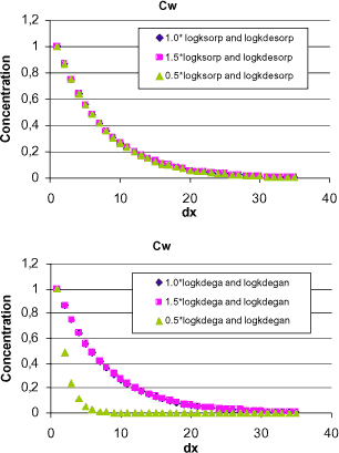
Figure 1.11 Sensitivity of concentration in bulk stream water, CW. the input parameters logksorp (and logkdesorp) and logkdega (and logkdegan) have been varied separately with 50 % of mean values to illustrate the model sensitivity.
The figure clearly shows a dependency on the degradation rates, whereas the influence from variations in sorption rates is not visible. It must be noted that all logk-values are negative and dividing a negative logk-value with a factor will increase the corresponding k-value. This is seen from the 0.5·logkdega (and 0.5·logkdegan) curves where a decrease in bulk water concentration is seen due to increased degradation rates.
When all input parameters are varied simultaneously it becomes rather complex to estimate variation patterns in the calculated output. A powerful tool to solve this task is multivariable partial least squares regression, PLS-R, where correlation patterns and significance of the individual input parameters can be found.
All pesticides
One way of investigating variability is by considering the individual variations of a set of physico-chemical properties in combination with the natural correlation patterns that exist between them. This is in fact
a crucial point, which will be mentioned in more detail later. The only two parameters that are available for a larger number of pesticides, namely 37, are the sorption equilibrium coefficient, logKd, and the
aerobic degradation rate, logkdega. For each of the 37 pesticides the stream model is run with the respective mean logKd and logkdega values, and since they are linked to the same pesticide they will be
inter-correlated.
To evaluate the variability in model output, output parameters are selected, which present large variations. From Figure 1.11 it is seen that the concentration at dx = 5 (500 m from the drain outlet) will be an appropriate choice. This concentration in the bulk water is denoted Cwdx5.
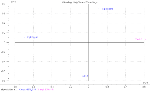
Figure 1.12 partial least squares regression, PLS-R, showing the influence of the normalised inter-correlated parameters logKd, logkdesorp, logkdega and logkdegan on the concentration in bulk stream water at a distance of 500 m from the drain outlet, Cwdx5. mean parameter values have been used for each pesticide.
In Figure 1.12 the result from the 37 model calculations are shown. Logksorp is constant and therefore is left out of the PLS, as it does not give any information. The inclusion of both logKd as well as logkdesorp will yield a more robust regression model.
The plot shows the loading weights, or significance, of the original input parameters in the first principal component, PC1 (abscissa), against the second principal component, PC2 (ordinate), with respect to the y-variable, Cwdx5. The variation in bulk water concentration is best described by original variables with large loadings weights in PC1, i.e. logkdega and logkdegan. logKd as well as logkdesorp have smaller loading weights in PC1 and accordingly only describe a smaller part of the variation in Cwdx5. This complements the findings of the simple analysis in Figure 1.11.
In Figure 1.13 a PLS-R plot of the influence of the pesticide concentration in sediment particles 500 m from the drain outlet, Ssdx5, is shown. 67 % of the variability in Ssdx5 is explained by the model. Contrary to the plot for Cwdx5 the variability is predominantly determined by the sorption process and to a lesser degree by degradation.
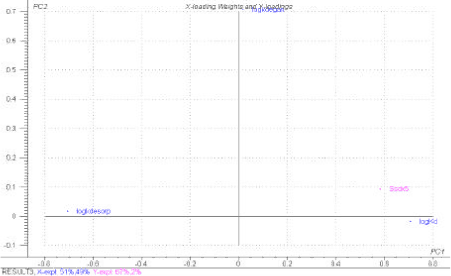
Figure 1.13 PLS-R, showing the influence of the normalised inter-correlated parameters logKd, logkdesorp, logkdega and logkdegan on the concentration in sediment particles at a distance of 500 m from the drain outlet, Ssdx5. mean parameter values have been used for each pesticide.
A further division of pesticides into two subgroups yields enhanced PLS models with a better explanation of the variability in e.g. Cwdx5. This is however beyond the scope of this work.
Bentazon and pendimethalin
In Figure 1.12 the variability in Cwdx5 has been investigated for correlated mean logksorp, logkdesorp, logkdega and logkdegan values. Further information is available on the variability of the individual parameters for
each pesticide, and by performing a MonteCarlo analysis this information can be utilised to investigate the influence on Cwdx5.
A PLS-R plot analogous to Figure 1.12 for bentazon and pendimethalin, which represent a hydrophilic and hydrophobic pesticide, respectively, is shown in Figure 1.14.
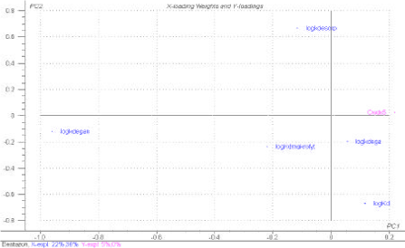
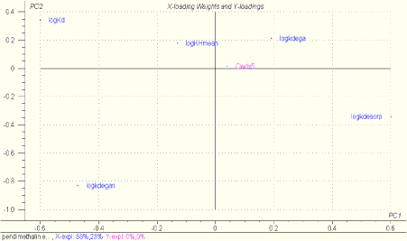
Figure 1.14 PLS-R plot showing the influence of the normalised parameters logKd, logkdesorp, logkdega and logkdegan on the concentration in bulk stream water at a distance of 500 m from the drain outlet, Cwdx5. The upper plot is for bentazon and the lower plot for pendimethalin. The parameter values assume normal distribution and have been selected randomly. Degradation and sorption parameters are therefore non-correlated. In the pendimethalin plot varying logKH values are included, and for bentazon a constant logKH is used. In the bentazon plot varying logKdmacro values are included, and for pendimethalin a constant logKdmacro is used. The plot is based on 100 MonteCarlo simulations of the stream model.
At a first glance the plots resemble Figure 1.12, but the calculations show that only 5 % of the variation in Cwdx5 is explained for bentazon and 0 % is explained for pendimethalin. The reason is that the results of the Monte Carlo simulated bulk water concentrations are based on random selection of individual input parameters, why the natural correlation patterns between physico-chemical properties are not accounted for. As such existing inter-correlation patterns between physico-chemical data, e.g. explained through high sorption affinity to suspended particulate matter implying low solubility and thereby low degradation rates in bulk water are not present in the above sensitivity analysis.
In this study uncertainty analysis is only performed for substance specific parameters. As in the natural environment, several conditions and additional unknown parameters add noise into the model, which decreases the correlation patterns of physico-chemical properties and exposure concentration. Site specific parameters such as the hydraulic water sediment exchange coefficient Ksedwat will have an influence on the substance concentration. This parameter is highly varying with varying hydraulic condition and important with respect to transport to the sediment.
When introducing the variability of a non-substance parameter, such as Ksedwat, in the stream model, the influence on the model output can become essentially different for the correlated substance parameters.
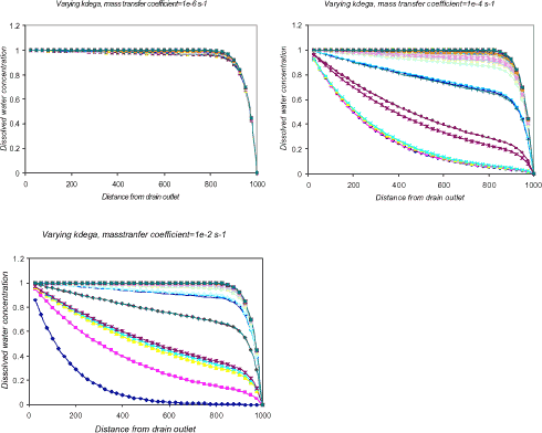
Figure 1.15 Bulk water concentration, Cw, at different distances from drain outlet. The influence of the aerobic degradation rate, kdega, is shown for three different values of the water sediment exchange coefficient, Ksedwat, namely, 1·10-6, 1·10-4 and 1·10-2 s-1.
From Figure 1.15 it is seen that there exists a parameter interval for Ksedwat where the influence from kdega becomes negligible. It is therefore important to identify such intervals and perform an uncertainty analysis for the appropriate parameters in each interval.
An important conclusion is that an uncertainty analysis of input parameters can not be performed by randomly selecting correlated parameters. They have to be selected by utilising the inherent relationships between them. Furthermore, using mean values reduce the influence from analytical and experimental errors, and gives more accurate inputs to the model. It is obvious that parameters that are determined with minimal standard deviation exhibit a more exact inter-correlation pattern with other parameters.
Based on the above introductory calculations an input uncertainty analysis can comprise the following
- Define the model system that is to be analysed.
- State input parameters, collect measured and/or literature data. Investigate if data display distribution function profiles, typically normal- or log normal distributions.
- Perform model calculations with selected input parameter mean values or ranges. Investigate if input parameter values describe model output variations, e.g. through PLS-R.
- Identify correlated input parameters, and predominant parameters, i.e. parameters that describe the variability of model outputs.
- Perform model calculations, which respect correlation patterns between parameters.
- Establish intervals for input parameter values that yield output values that exceed critical values. Estimate the probability for exceeding critical output values.
1.5 Guidelines for uncertainty estimates of stream and pond models
In the previous sections the influence of parameter uncertainty on the stream model with respect to the water phase and sediment has been investigated. This has been done by varying the parameter values and running the quasi-stationary and non-steady-state model systems, respectively. Such calculations form the optimal basis for establishing qualitative relationships between model output and input parameter values.
It is, however, difficult to derive simple quantitative or functional relationships based on the calculations, in order to establish guidelines, which are directly applicable as support in uncertainty estimation.
For this purpose simple equations will be derived below to describe the system sensitivity for different input parameter values. The equations are validated with the above analytical calculation. The stream and the pond will be treated separately having focus on both the water and sediment concentration.
The uncertainty of the modelling result due to the uncertainty of a single input parameter is obviously strongly related to the actual influence on the modelling result from that specific parameter value. In other words if a parameter value is not important for the final modelling result then the uncertainty of the actual parameter value will never be important for the model validity. The influence of one parameter often depends on other parameter values. In this way parameter 1 may only be important if parameter 2 is “high” also, so if parameter 2 is “low” then the uncertainty of parameter 1 will not be important. These interacting relationships are disclosed in this paragraph ending up in a guideline for the uncertainty analysis of the stream and pond systems.
Special relationships exist however, for the Henrys Law Constant (Hg) in the stream model, where neither the air phase nor the water phase represent the dominating resistance for evaporation as shown in section 1.3.3. Another parameter of special concern is the diffusion coefficient for the transfer from the water column in the pond model where the conventional parameterisation is to use the molecular diffusion coefficient.
1.5.1 The stream model
The water and sediment depth (hw and hsed) and the width of the stream (w) will be assumed constant in the following equations.
The hydraulic retention time in the stream water is defined as:
![]() (1.60)
(1.60)
where L is the length (m) of the stream and Q is the flow rate (m³/s). The concentration drop for a 1st order removal mechanism in the stream is given by an exponential functional relationship. As long the change in concentration is relatively small a Taylor series expression can be used as:
![]() (1.61)
(1.61)
The 1st order removal constant K for different mechanisms in relation to the dissolved water concentration in the water column is shown in Figure 1.16 and Figure 1.17.
The hydrodynamic mass transfer is characterised as the mass of substance transferred to the system during the retention time
![]() (1.62)
(1.62)
where cw,o is the dissolved water concentration at the inlet to the stream and Vtot is the total water volume in the stream. This mass value can be referred to as a reference mass.
The mass removed by adsorption to suspended solids is characterised as the maximum mass removal from the stream during a period equal the retention time as
![]() (1.63)
(1.63)
where k1w is the adsorption coefficient to the suspended solids (m³/(kg·s)) in the water column and CP is the concentration of suspended solids in the water column (kg/m³).
The mass removed by degradation is characterised as the maximum mass removal from the stream during a period equal the retention time as
![]() (1.64)
(1.64)
where kw,deg (1/s) is the first order degradation coefficient in the water column. The mass removed by adsorption to macrophytes is characterised as the maximum mass removal from the stream during a period equal the retention time as
![]() (1.65)
(1.65)
where k1m is the adsorption coefficient to the macrophytes solids in the water column (m³/(kg·s)) and CM is the macrophytes concentration (kg/m³). The mass removed by transfer to the sediment is characterised as the maximum mass removal from the stream (where the pore water concentration (sw) is zero) during a period equal the retention time as
![]() (1.66)
(1.66)
where ksed/wat is the mass transfer coefficient (m/s) for the sediment/water column exchange.
The mass removed by evaporation is characterised as the maximum mass removal from the stream during a period equal the retention time as
![]() (1.67)
(1.67)
where Kw (m/s) is the mass transfer coefficient for the air/water exchange.
The total mass transfer potential is characterised simply by adding all the mass transfer characteristics together as
![]() (1.68)
(1.68)
There is a hierarchy of parameter influence on the dissolved water concentration and the following decision tree will sum up the relationships related to the test equations above.
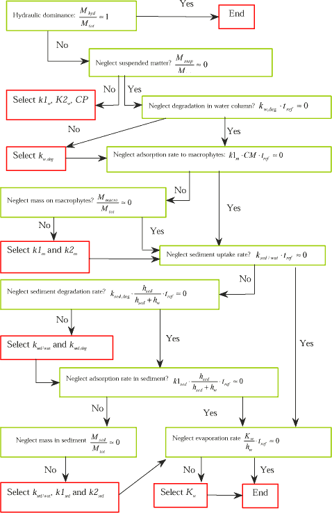
Figure 1.16 Decision tree for identification of parameters, which may have influence on the calculated dissolved water column concentration.
The concentration value in the sediment (sw) is also one of the modelling result, which needs to be considered. Processes, which have an influence on the cw, value will also have influence on the sw value because the transfer rate from the water column to the sediment will be affected. The partitioning between dissolved and adsorbed fraction in the sediment will always be an important factor because of the high content of adsorption sites in the sediment.
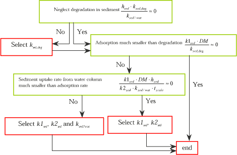
Figure 1.17 Decision tree for identification of parameters, which may have influence on the calculated sediment layer concentration (both dissolved and adsorbed).
1.5.2 The pond model
In the pond the reference volume of water is selected to be the volume per unit area, thus the water depth hw. The mass of substance in this volume is
![]() (1.69)
(1.69)
The retention time is defined of the half-life time in the water column only due to removal by degradation in the water column in case of no other transfer mechanism from the water column. This removal is described in the following equation
![]() (1.70)
(1.70)
Combining Equations 1.36 and 1.37 the following equation for the retention time is derived:
 (1.71)
If a transfer mechanism is unable to remove a considerable amount of mass from the water column during the time period tref then it is true that this mechanism is not important for the calculated water column concentration level.
The maximal possible amount of substance mass adsorbed to the macrophytes is given as
![]() (1.72)
(1.72)
The mass of substance taken up by the sediment from the water column can only be calculated using the full numerical solution in the model, however, some limit values can be identified in a simple way and they can form a guide for the possible sources of uncertainty. In the context the first characteristic parameter is the upper limit for the sediment accumulation which will be derived in the following. In case of constant water concentration and no degradation in the sediment the it is possible to derived a equation for the mass of substance in the sediment based on the analytical solution of the sediment transport equation (Sørensen et al. 2001) as
![]() (1.73)
(1.73)
where R is the retardation factor and defined as: ![]() , where Θ is the porosity and σ is the bulk density. The porosity and the bulk density will clearly depend on the specific sediment. But, for highly organic content realistic values are: Θ = 0.8 and σ = 1.5 kg/l. So, e.g. for pendimethalin as given in Ref. (eksperiment-rapport), where a realistic Kd for the pond sediment is around 700 the corresponding R value will be around 1300. This equation represent the upper limit of the sediment uptake because it is assumed that cw is constant during time and no degradation. In reality the cw value will decrease due to the removal and in the sediment the amount of substance will be reduced by degradation.
, where Θ is the porosity and σ is the bulk density. The porosity and the bulk density will clearly depend on the specific sediment. But, for highly organic content realistic values are: Θ = 0.8 and σ = 1.5 kg/l. So, e.g. for pendimethalin as given in Ref. (eksperiment-rapport), where a realistic Kd for the pond sediment is around 700 the corresponding R value will be around 1300. This equation represent the upper limit of the sediment uptake because it is assumed that cw is constant during time and no degradation. In reality the cw value will decrease due to the removal and in the sediment the amount of substance will be reduced by degradation.
The upper limit for removal in the sediment by degradation can be calculated by assuming steady state conditions. If the water concentration is assumed constant then after a sufficient long time period the will exist a steady state flux into the sediment equal to the degradation in the sediment. At these conditions the degradation in the sediment will be at a maximal level. Thus, the upper limit for the rate of substance removal by degradation in the sediment can be derived by using the equation for steady state conditions. The removal rate under steady state conditions during the time period tref is
![]() (1.74)
(1.74)
We can now set up a decision tree to identify the most important parameters for the calculation of the dissolved water column concentration as seen in Figure 1.18.
Figure 1.18 Decision tree for uncertainty analysis of the pond model.
1.6 Soil model in relation to drain flow transport
The catchment area for the stream model is soil cultivated for agricultural purposes. The soil compartment thus defines the pesticide input concentrations and flows to the stream.
The registration model comprises a model, MIKE SHE, designed for natural hydrologic systems. In this study MIKE SHE has been adapted for two typical Danish catchments:
- Lillebæk in Fyn
- Odder Bæk in Northern Jylland
MIKE SHE comprises descriptions and solutions to hydraulic dynamics and substance transport and fate in unsaturated and saturated zones in soil as well in groundwater. The basic governing equations for simulating fluxes of water in the unsaturated zone are Richards' equations and the three dimensional fluxes of water in the saturated zone is the Darcy equation. An in depth description of the water movement can be found in DHI MIKE SHE user manuals (DHI,?).
Once the hydraulic balance of the system is known the substance transport and fate in the soil can be calculated, based on the convection-dispersion transport model for a sorbing and degradable species, according to the substance balance equation
![]() (1.75)
(1.75)
where Cw is the concentration of dissolved pesticide in the soil pore water, t is the time, r = (Θw + KF Xsoil) is the retention coefficient, based on the Freundlich equilibrium partitioning coefficient, KF, soil density Xsoil and soil porosity, w. Dsoil disp. is the dispersion coefficient, z is the (vertical or diagonal) transport length, q is the bulk flow and ksoil degr. is the 1st order degradation rate.
Equation 1.75 applies for both the unsaturated and saturated zone (vertical flow). Furthermore in the unsaturated zone preferential flow or macropore flow, can be important in many soil types and can be incorporated in addition to the Richards' type flow. Macropore flow is dominated by advection and assumes a secondary pore domain through which water is routed separately. Dissolved substances will be transported in the macropores and an exchange between the macropores and the surrounding bulk porosity (or matrix porosity) is possible.
The macropore flow is accounted for by dividing the infiltration water, e.g. from precipitation, into two parts; one part that flows through the soil matrix and another part which is routed directly to the groundwater Table (bypass flow). The bypass flow is thus calculated as a fraction of the infiltration water.
Typical values for macroporosity are around 2% at the soil surface, for clay and loamy soil, and decreasing exponentially with depth. The influence on substance behaviour is an earlier substance breakthrough compared to flow through the soil matrix. The less permeable soil structure, e.g. for clay, the higher water flow through macropores, which implies lower concentrations in the soil water but higher substance flux through the soil.
Sorption processes cover a number of geochemical and chemical reactions. If these reactions occur sufficiently fast compared with the water flow velocity they can be described by an equilibrium sorption isotherm, otherwise they have to be described by a kinetic sorption isotherm. Sorption in soil can usually be considered to have reached equilibrium, special attention may however be taken when macroporous transport is dominant.
If sorption equilibrium prevails the sorbed pesticides concentration can be found according to the Freundlich sorption isotherm. It describes a non-linear relationship between the amount of substance sorbed onto the soil material and the aqueous concentration of the substance. Issues concerning the concentration dependency of KF are treated in section 1.3.1. Essential for the substance concentrations calculations in the soil is that the pesticide concentration is very low and often (if not always) below the experimental concentrations where the equilibrium coefficient, KF, has been found. The optimum approach to calculate sorbed pesticide in order to avoid serious overestimation of sorption, is therefore to extrapolate linearly in the low concentration interval
![]() (1.76)
(1.76)
where Cs is the concentration of sorbed substance in mg pr. kg. dry matter.
When sorption and degradation are included in MIKE SHE they are applied as Koc and aerobic degradation rate, respectively. The KF and DT50 values representative for the different depths in the soil profile are then calculated from measured and estimated organic content, and assumptions on oxygen and water content according to the guidelines stated in FOCUS (2000).
MIKE SHE allows for flow through drains in the soil. Drainage flow occurs only in the top layer of the groundwater model when the water table is above the position of the drains. When a real climate profile is employed in MIKE SHE the precipitation, temperature and other processes will vary and accordingly the groundwater table will vary. This will result in periods with flow and no flow through drains.
1.6.1 Sensitivity analysis of worst-case scenario
When the soil surface layer has been contaminated MIKE SHE can be used to simulate time series of output pesticide concentrations from the soil, which will act as input (boundary conditions) to the stream model. Two cases can be considered
- Transport through the unsaturated zone into the drain.
- Transport through the unsaturated and saturated zone (leaching/infiltration).
Both cases describe a concentration peak moving in the soil system towards and into the stream. Situation 1) can be detected faster in the stream compared to situation 2) and the maximum concentration will be higher.
When risk assessment of pesticides in surface waters is performed a conservative approach is to consider a worst case scenario with respect to pesticide input to the recipient. Such a scenario can be described with a flow of maximum pesticide concentration from the soil and/or a maximum concentration gradient in time entering the recipient. For the catchment system this will imply the presence of macropore flow and drains, corresponding to situation 1) above.
This worst case situation can be studied by performing a focused uncertainty analysis of the MIKE SHE catchment systems. It is however not feasible to include the entire Lillebæk or Odder Bæk system, as one single simulation lasts hours.
A part of the MIKE SHE Lillebæk catchment model system, comprising 11 grids each 50 times 50 m, has been isolated. The sub-catchment is dominated by drainage, which therefore can be considered to be the only substance source to the stream on this location.
A sensitivity analysis is performed with a climate profile for the period from 1997 to 2000. A spraying scenario is defined as an application once, with 0.56 mg/(m²s) for 1 minute, in May 1997 on each of the 11 grids.
In Figure 1.19 the dissolved bentazon concentration in the drain, based on the mean values stated in Table 1.2, is shown. The concentration in the drain has been weighted according to the individual flow rates and concentrations in the grids. When no drain flow is present in a grid, either due to groundwater below drain or negligible soil flow, the drain concentration is zero.
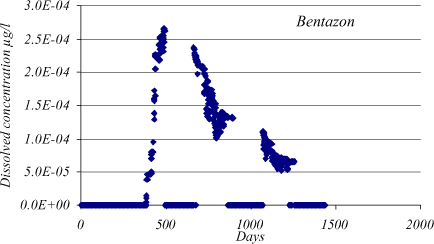
Figure 1.19 Bentazon drain concentration for a Lillebæk sub-catchment consisting of 11 grids. Bentazon is applied in May 1997 on all grids. Mean kdeg and Kd values stated in Table App5.2 have been used. The time periods with concentration zero occur when the drain flow is zero.
When the time intervals with zero flow are omitted the concentration trend in Figure 1.20 is found.
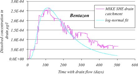
Figure 1.20 Bentazon drain concentration for a Lillebæk sub-catchment consisting of 11 grids. Mean kdeg and Kd values stated in Table App5.2 have been used. The time periods with concentration zero have been omitted. A fitted log-normal curve is shown.
The bentazon breakthrough at the drain from the unsaturated zone is almost immediate and the maximum concentration, Cmax, is about 2.610-4 µg/l after approximately tmax = 110 days. Calculations from a simple numerical solution of Equation 1.42 show that the concentration from transport through the unsaturated and saturated zone is negligible after 110 days. It peaks around 2000 days and the maximum concentration as well as the concentration gradient is very much smaller than for the drain.
The time for maximum concentration in the drain is tmax. Sorbing substances spend 1/r as much time in the dissolved phase as a identical non-sorbing substances, which implies a delay in the soil matrix with a factor of r. For hydrophilic substances r is close to unity, and no delay is observed in the soil matrix.
For bentazon r = 1.07, and the peak is around 110 days. For more hydrophobic substances there will be a linear dependency between tmax and r according to
![]() (1.77)
(1.77)
For the more hydrophobic pendimethalin the time for maximum concentration is a factor of 80 (retention factor, r = 80) longer than for bentazon, and the peak in the drain will therefore occur after approximately 9000 days or 24 years.
tmax is, however, also dependent on kdeg and Equation 1.77 is therefore only valid for the mean bentazon kdeg value.
To investigate the influence of kdeg and Kd on tmax and Cmax a sensitivity analysis is made for the MIKE SHE drain catchment, where Kd and kdeg values are selected to cover a “grid” of 10 x 10 values. Due to a limited simulation time period of approximately 500 days Kd is cut of at approximately 3, depending on kdeg, corresponding to approximately r = 5 and tmax = 500 days.
It is important to note that such an analysis does not conflict with the guidelines that are previously stated. This is a sensitivity analysis and does not reflect on correlation patterns between parameters, but rather considers the model output for an “entire” input parameter space.
In Figure 1.20 the tmax dependency on kdeg and Kd is shown and in Figure 1.21 the Cmax dependency on kdeg and Kd is shown as a result of 100 simulation runs of the Lillebæk sub-catchment system.
Figure 1.21 Time for reaching maximum dissolved pesticide concentrations in the drain for varying kdeg and Kd values.
tmax is linearly related to Kd and curve fittings show a polynomial relationship to kdeg.
![]() (1.78)
(1.78)
where a to e are constants found from the curve fittings.
Figure 1.22 Maximum dissolved pesticide concentrations in the drain for varying kdeg and Kd values.
In order to estimate Cmax and tmax in the drain, three different substance classes can be distinguished.
Class A:
kdeg > 3.58·10-7 s-1 (t½ < 22 days for r ≈ 1):
Cmax is negligible (below 10-6 µg/l) for all Kd values, and no peak concentration is discernible. Class A points are not shown in Figure 1.20 and Figure 1.21.
Class B:
1·10-7 < kdeg < 3.58·10-7 (22 days < t½ < 80 days):
Kd > 1: Cmax ≈ 0.
Kd < 1: Cmax can be fitted to a polynomial relationship with respect to Kd, and a linear relationship with respect to kdeg (only two data points), according to
![]() (1.79)
(1.79)
Class C:
kdeg < 1·10-7 s-1:
Cmax can be fitted to an exponential expression with respect to Kd and kdeg, according to
![]() (1.80)
(1.80)
When Kd is larger than approximately 3, tmax is larger than 500 days, which is the time limit for this specific drain study. f to o are constants found from the curve fittings.
37 different pesticides have defined Kd and kdeg values according to PATE (2001). 23 of these can be categorised in class A, 13 in class B and 1 in class C. With the given application rate for the Lillæbæk catchment only 3 pesticides have Cmax values different from zero, i.e. bentazon, clopyralid and haloxyfopethoxyethylester. All are in class B with Kd below 1.
When known mean values and standard deviations for kdeg and Kd are available for a pesticide, the probability for a given Cmax value can be found. In the model calculations it is required that the parameter values are correlated.
In Figure 1.20 is also shown that the dissolved concentration in the drain as a function of time, can be approximated with the log-normal function
 (1.81)
where Mappl is a constant expressing the application rate of the pesticide. 0.56 mg/(m²·s) is the calibration application rate. t is the time in days and K is a fitted value for defining the standard deviation of the population of log(t). K is a function of kdeg and Kd and assumes values in the range from 0.5 to 1.2 for the considered parameter intervals.
In Figure 1.23 a log-normal distribution is shown. When applying a limit value (LV) the time interval (Δtcrit) for exceeding the limit value can be found from Equation 1.81 to be
![]() (1.82)
(1.82)
where
![]() (App5.83)
(App5.83)
is the upper time limit, and
![]() (1.84)
(1.84)
is the lower time limit.
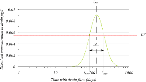
Figure 1.23 log-normal concentration distribution with indicated time interval (tcrit) for exceeding a given limit value (LV).
The equations for defining a worst case scenario with respect to emissions from the soil to the stream have now been set up. Equations 1.82, 1.83 and 1.84 yield the maximum concentration in the drain and the time for reaching this concentration, respectively. The approximated log-normal fit of the concentration time trend permits an estimation of if and how long a given limit value is exceeded in the drain water.
Figure 1.24 Decision tree for calculating the maximum dissolved pesticide concentration in drain water (Cmax), the time for obtaining this concentration (tmax) and the time interval (tcrit) for exceeding a given limit value (LV) in drain water. The drain scenario is considered to be worst case with respect to peak concentrations in the outlet from agricultural soils to surface waters.
The stream receives the drain water and the steady-state concentration level is proportional to the concentration in the influent drain water. From the curve shown in Figure 1.23 and by dividing with the conversion factor to the stream, which is a function of various process parameters, the time for exceeding a given limit value in the stream water can be found.
Version 1.0 Maj 2004, © Danish Environmental Protection Agency