Scenarios and Model Describing Fate and Transport of Pesticides in Surface Water for Danish Conditions
3 Changes from Calibrated Catchments to Scenarios
3.1 Lillebæk stream
3.2 Odder bæk
3.3 The pond scenarios
3.3.1 Geomorphology
3.3.2 Pond Type around Odder Bæk
3.3.3 Pond Type around Lillebæk
3.3.4 Conclusions regarding types of ponds
3.3.5 Dimensions of the Ponds
3.3.6 Biological structure of the pond
3.3.7 Implementation of the pond in the Lillebæk model setup
3.3.8 Implementation of the pond in the Odder Bæk model setup
The basic parameterisation of the models implemented are described in the calibration report, Styczen et al. (2004a). The model systems are described in the User Manuals for MIKE SHE, MIKE 11 and in the technical documentation, Styczen et al. (2004c).
However, with the change of the models from “real” conditions to scenarios, a number of changes are made in the way, the models are parameterized.
For all scenarios, the agricultural area of the scenarios is cropped with one crop only, and the total agricultural area is sprayed on the same day(s) with the pesticide. Non-agricultural areas or areas with permanent grass remain as they are, and are not sprayed in the scenarios.
As mentioned in Section 2.2, although the permanent grass area appears large in the sandy catchment, similar permanent grass areas are found in other sandy areas of Jutland. For the counties of Sønderjylland, Ribe, Ringkøbing, Viborg and Nordjylland (dominated by sandy soils), the percentages of permanent grass are between 14,5 and 18,2. The 12,9% are therefore not unrealistic, in fact it is slightly less than average.
A decision to include the permanent grassland as arable agricultural land would affect the simulations considerably, as these grassed areas usually are found near streams, in areas with high groundwater, and thus highly susceptible to leaching. Additionally, they will be close to the stream, and therefore limit the area from where drift can occur. Usually, these soils are not suitable for cropping.
3.1 Lillebæk stream
For Lillebæk catchment, the main change is that the piped length of the stream is turned into an open stream. Pesticide can thus enter the stream through drift and dry deposition to a much larger extent than in reality. No trees are included in existing buffer zones (although they exist in reality), but the width of the natural buffer zones are kept.
3.2 Odder bæk
Odder Bæk is implemented as it exists in the calibrated version.
3.3 The pond scenarios
No ponds were monitored and it was therefore not possible to calibrate directly on existing conditions. However, a pond was placed within each scenario, inheriting as many of the properties of the scenario as possible. In the following sections, the intentions of the pond scenarios are outlined.
The objective of the pond scenarios is to evaluate the situation of a typical sensitive stagnant water body, which is very abundant in the Danish agricultural landscape. There is a high awareness in Denmark of the importance of the small water bodies in relation to bio-diversity and protection of endangered species. The stagnant nature of the water body and the size means that the concentration of pesticides may become relatively high and accumulation may occur dependent on the properties of the pesticide in question. The present scenario used for registration is a pond.
3.3.1 Geomorphology
Geomorphologically, Lillebæk represents moraine clay from the second last and, in the northern part, also the last ice age. Odder Bæk represents a melt water stream terrace and peripheral moraine. It is a moraine landscape from the last ice age. Geomorphologic formations such as moorland plain and hill islands (Western Jutland), uplifted sea bottom (Northern Jutland) and the more clayey soils found on parts of Sealand and further south are thus not represented.
3.3.2 Pond Type around Odder Bæk
The pond type found in the surroundings of Odder Bæk is peat bog. In this area, the soil is very sandy, or in some parts organic, and the infiltration is expected to be great. Below the soil is a 5-7 m thick layer of melt water deposits, on top of drift deposits (15 m thick). The drift deposit is expected to constitute the bottom of the sediments in the peat bog. Below the drift deposit, another melt water sand deposit and another drift deposit, but these are saturated by primary groundwater and are expected to be of less importance for the dynamics of the pond.
The groundwater potential is relatively close to the surface of the pond, and it is expected to be the governing factor for water movement to (and from) the pond. This is consistent with the fact that peat is formed in places with a relatively constant water level. Due to the fact that the surface soil is very sandy and the infiltration high, the amount of surface runoff is expected to be small. The percolated water will either collect on top of the drift deposits and run to the bog or possibly infiltrate to the groundwater level, which then controls the water level in the bog. The dynamics of this pond type is shown in Figure 3.1.
A representative size of small bogs appears to be 300-500 m² (Agger and Brandt, 1986).
Some information was received from the county of Ringkøbing concerning new (artificial) ponds recently constructed. While these are not bogs as such, the general pattern may not be very different. Farmers tend to choose low areas, which are moist and not well suited for cropping, and the general size are about 300-500 m².
Figure 3.1 Diagram of a bog and the geology surrounding it. Note the high groundwater level.
Figur 3.1 Diagram af et vandhul og geologien omkring den. Bemærk det høje vandspejl.
3.3.3 Pond Type around Lillebæk
The ponds around Lillebæk are kettle holes. They are all found on moraine clay. The surface soil is generally coarse or fine sand-mixed clay (types 4 or 5). Below this, a moraine clay layer of approximately 5 m depth is found, in which the kettle hole probably is formed. Below the moraine clay, about 30 m of melt water deposits are found.
The groundwater potential (primary groundwater) is somewhat below the water level in the ponds and the ponds are not expected to be particularly influenced by groundwater. The clayey surface and the upper drift deposits have a low permeability, which makes it difficult for the water to infiltrate. It is therefore probable that surface runoff (or perched groundwater present in the upper layers due to local impermeable layers) will dominate the water flow to the pond. There may be some infiltration from the pond to lower layers.
This pond type appears to dominate east Denmark, except on the more clayey soils, where marl-pits are frequent. 200-400 m² appear to be a representative size for these small lakes (Agger and Brandt, 1986). The dynamics of this pond type is shown in Figure 3.2.

Figure 3.2 Diagram of kettle hole and the geology of the surroundings. Note that the water table is below the bottom of the lake.
Figur 3.2 Diagram af et dødishul og geologien omkring det. Bemærk at vandspejlet er under søens bund.
3.3.4 Conclusions regarding types of ponds
There is little doubt that the two types of ponds, which relate to the geomorphology of the test areas, are rather typical pond types for Denmark. They also have a distinctly different hydrology. It is, however, not documented that they are the only typical pond types in the country. The advantages of choosing these two pond types for simulation are that:
- the necessary parameters have been generated through the general simulation of the test areas
- the ponds are representative of common Danish ponds, and do represent distinctly different types of hydrology (strong groundwater domination and strong surface-domination)
3.3.5 Dimensions of the Ponds
A number of criteria for design of the ponds have been suggested by EPA and the steering group:
The ponds must be small. On sandy soils, the available material shows a typical size of 300-500 m², on sandy loam, the size is about 200-400 m². The depth of the pond is determined by the requirements that:
- it should not dry out, and
- a typical variation of the water level in small ponds is about 1 m.
A depth at 0.5 m at minimum would then mean a typical depth of 1.5 m during the wet parts of the year. The variation in depth is then from 0.5-1.5 m.
The topography follows the landscape in the catchment.
3.3.6 Biological structure of the pond
For Danish lakes it is well documented that the input of nutrients is important for the biological structure of the ponds (Figure 4.10) and the same is assumed for the ponds in agricultural catchments. To take this structural differences into account it was decided to implement both macrophyte and phytoplankton dominated pond as scenarios. In addition to the biomass of macrophytes these scenarios also have implication for the concentration of suspended matter in the water column and consequently for the sorption of the pesticides. In addition, the concentration of suspended matter might affect the light penetration in the water and thereby the rate of the photolytic decay of pesticides. Finally it is assumed that the sediment in the phytoplankton dominated ponds is anoxic and the biodegradation consequently anarobic. For a further discussion of parameterization of the different ponds scenarios see Sections 4.5, 4.6 and 4.7.
3.3.7 Implementation of the pond in the Lillebæk model setup
The pond model for Lillebæk was set up for the subcatchment area in Figure 3.3. Due to the small size of the pond (app. 200-300 m²), a smaller grid size of 25 X 25 m² was used for the pond model compared to the original model (50 X 50 m²).
The pond was set up in MIKE 11 as a single 25 m long stream branch with a 10 m wide cross-section, see Figure 3.4. Ground elevation is 48 m at the location of the pond and the pond was assumed to be 1.5 m deep. Water is assumed to leave the pond through an outlet but may also infiltrate through the lake bottom to lower layers. The outlet for Lillebæk pond was modelled by adding a weir to the branch with a crest elevation of 47.75 m allowing water to leave the pond before the water level reaches ground elevation.
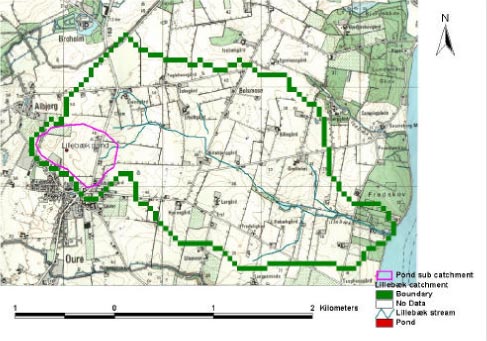
Figure 3.3 Pond location in Lillebæk catchment.
Figur 3.3 Placering af vandhul i Lillebæk-oplandet.
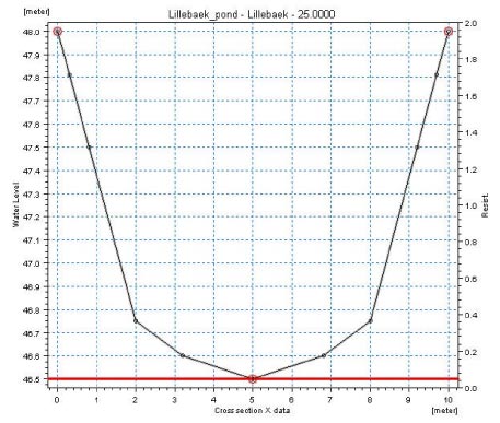
Figure 3.4 Pond cross-section in MIKE 11 for the Lillebæk pond scenario.
Figur 3.4 Tværsnit af Lillebæk-scenarie-vandhullet i MIKE 11-modellen.
Flow into the pond in this catchment consists of drain flow alone. Moreover no recharge from the aquifer will occur as groundwater levels are between 2-3 m below ground surface throughout the year. An area around the pond of app. 0.12 km² was assumed to contribute to the pond with drain flow when groundwater levels are higher than 1.5 m below ground elevation. The drain areas contributing with flow into the pond are delineated in Figure 3.5. The groundwater levels at the subcatchment boundary were extracted from the regional Lillebæk model in order to capture the dynamics and groundwater levels correctly. This also ensures that drain flow into the pond will be limited to the wet season from October to May.
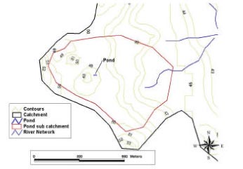
Figure 3.5 Catchment area for Lillebæk scenario pond. Note that only part of the area drains towards the pond.
Figur 3.5 Oplandsareal til Lillebæk scenarie-vandhul. Bemærk at kun en del af arealet dræner mod vandhullet.
In order to maintain a minimum water level in the lake of 0.5 m, the leakage coefficient of the pond bottom lining was adjusted to a value of 5 . 10-7 sec-1.
The water level variation in the pond and inflow to the pond in 1990 is illustrated in Figure 3.6. The pond is surface water controlled as illustrated by the very dynamic inflows to the pond.
Figure 3.6 Simulated pond water level (m) and inflow to pond (m³/s)i Lillebæk scenario.
Figur 3.6 Simuleret vandniveau (m) i og tilstrømning (m³/s) til Lillebæk-scenarie-vandhul.
3.3.8 Implementation of the pond in the Odder Bæk model setup
The pond model for Odder Bæk was set up for the subcatchment area in Figure 3.7. The same grid size of 25 X 25 m² used for the pond in Lillebæk was used for the Odder Bæk pond model.
The pond was set up in MIKE 11 the same way the Lillebæk pond was modelled. The pond size is somewhat larger app. 400 m², which was set up by defining a 40 meter branch and cross-sections similar to the ones used for Lillebæk. Ground elevation is 24.25 m at the location of the pond and the pond was assumed to be 1.5 m deep. Water is assumed to leave the pond through an outlet but may also infiltrate through the lake bottom to the lower layers. The outlet for Odder Bæk pond was modeled by adding a weir to the branch with a crest elevation of 24 m allowing for water to leave the pond before the water level reaches ground elevation.
Figure 3.7 Pond location in Odder bæk catchment.
Figur 3.7 Placering af vandhul i Odder bæk-oplandet.
Flow into the pond in this catchment consists of groundwater flow alone. The topsoil is coarse so water will infiltrate rather than run off on the surface and the groundwater table is close to the surface during the wet season. The groundwater levels at the sub-catchment boundary were extracted from the regional Odder Bæk model in order to capture the dynamics and groundwater levels correctly. A similar water level variation is expected to occur in the pond assuming the pond and underlying aquifer is in contact.
In order to maintain a minimum water level in the lake of 0.5 m and model the groundwater controlled water level variation in the pond, the leakage coefficient of the pond bottom lining was adjusted to a value of 5 . 10-6 sec-1.
The water level variation in the pond and inflow to the pond in 1995 is illustrated in Figure 3.8. The pond is groundwater controlled as illustrated by the simulated in- and outflows for the pond.
Figure 3.8 Simulated pond water level (m) and groundwater exchange (m³/s) in the Odder Bæk scenario pond.
Figur 3.8 Simuleret vandniveau og grundvandsudveksling i Odder Bæk scenarie-vandhullet.
Version 1.0 Maj 2004, © Danish Environmental Protection Agency