Scenarios and Model Describing Fate and Transport of Pesticides in Surface Water for Danish Conditions
4 Parameterisation of Sub-components
4.1 Growth curves and deposition on soils
4.2 Wind drift
4.3 Dry deposition
4.4 Calculation of effective pesticide dose on the soil
4.5 Adsorption to macrophytes
4.6 Adsorption to suspended matter
4.7 Sediment in streams and ponds
4.1 Growth curves and deposition on soils
Plant growth information appears in the model in two ways. Information on root depth and leaf area index over time determines the calculation of transpiration. Furthermore, the growth stage and percentage cover at a given time determines the amount of deposition on the soil surface. For the calibration of the water model, values from (Plauborg and Olesen, 1991) for the agricultural crops were used for Leaf Area Index and Rooting Depth. For deposition of pesticide on soil, the results from Jensen and Spliid (2003) are used for vinter wheat, spring barley, potatoes and sugar beets. For other crops, the recommendations by FOCUS (2000) are used. Tables illustrating these relationships are given in Appendix B.
Figure 4.1-Figure 4.4 compares the values of Jensen and Spliid (2003) and FOCUS(2000) for the four crops where both data sets are available.
Figure 4.1 Deposition of pesticide on soil under winter wheat, as estimated by Jensen & Spliid (2003) and FOCUS (2000).
Figur 4.1 Deposition af pesticid på jorden under vinterhvede, bestemt af Jensen & Spliid (2003) og FOCUS (2000).
Figure 4.2 Deposition of pesticide on soil under spring barley, as estimated by Jensen & Spliid (2003) and FOCUS (2000).
Figur 4.2 Deposition af pesticid på jorden under vårbyg, bestemt af Jensen & Spliid (2003) og FOCUS (2000).
Figure 4.3 Deposition on soil under sugar beet, as estimated by Jensen & Spliid (2003) and FOCUS (2000).
Figur 4.3 Deposition af pesticid på jorden under sukkerroer, bestemt af Jensen & Spliid (2003) og FOCUS (2000).
Figure 4.4 Deposition under potatoes, as estimated by Jensen & Spliid (2003) and FOCUS (2000).
Figur 4.4 Deposition af pesticid på jorden under kartofler, bestemt af Jensen & Spliid (2003) og FOCUS (2000).
4.2 Wind drift
At present, the Ganzelmeier values for drift are used in Denmark when determining the size of buffer zones required in pesticide registration (BBA, 2000). The values are based on drift experiments carried out in Germany under wind speeds that are common for the continental climate. These wind speeds are relatively low (ca 2 m/s in average for field crops). The Ganzelmeier values are 95% percentile values of individual observations. This means that 95% of the individual measurements have resultet in drift values less than the Ganzelmeier values, which are 2-3 times higher than the average values. The Ganzelmeier values are thus kind of worst case values for the specified wind conditions.
In order to investigate the 2 m/s-assumption, average wind speeds data from the Danish research station “Flakkebjerg” were investigated. Figure 4.5 shows the wind profile over the day, based on average values from May and June, 1991 to 2000.
Figure 4.5 Wind profile at Flakkebjerg research station, average values for the months may and June (1991-2000). The values at 10 m's height are measured, while the speed at 2 m's height is calculated. The low velocities during the night are typical of a coastal climate.
Figur 4.5 Vindprofil på Flakkebjerg forsøgsstation, gennemsnitlige værdiger for månderne maj og june (1991-2000). Værdierne i 10 m's højde er målte mens hastigheden i 2 m's højde er beregnet. De lave værdier målt om natten er typiske for et kystklima.
It is quite common that farmers spray very early in the morning, but even here, the average wind speed is higher than 2 m/s. Assuming that the drift increases linearly with the wind velocity at velocities above 1 m/s. Spraying at wind velocities of 3-4 m/s will result in drift values which, in average, are at the level og the Ganzelmeier values. The figure shows that wind velocities of 3-4 m/s are close to the actual average values found in Denmark during the spraying period in spring.
A careful farmer will be able to carry out his sprayings under more favourable wind conditions, particularly sprayings where the timing is less critical and may take place within an interval of perhaps a week. For many sprayings, however, the timing is critical and only allows spraying within an interval of few days, or alternatively a higher dosage is required.
It was therefore agreed to interpret the Ganzelmeier 95 percentile values as average values for Danish conditions. In the FOCUS surface water scenarios, a special procedure is used for wind drift if more than one application of pesticide is carried out because the drift calculation is interpreted as a 90 % percentile. Such a procedure is not implemented here, as the percentile is interpreted as the average condition.
In the scenarios, the wind is always blowing perpendicular to the stream. This issue was discussed at length. This assumption is an overestimation compared to the general situation, but not necessarily to the conditions during a single spraying event.
Relationships were established between drift and distance from the stream for agricultural crops, apple trees and pine trees. These are based on the Ganzelmeier values, but interpreted as average conditions. An example of this is shown in Figure 4.6. All relations used are described in Appendix C. Winddrift is added over a period of 30 minutes for the whole catchment.
Figure 4.6 Fitted and measured relationship between distance from sprayer and drift applied for agricultural crops.
Figur 4.6 Beregnet og målt sammenhæng mellem afstand og drift anvendt for landbrugsafgrøder.
The input to the stream attributable to spray drift and dry deposition is dependent on the width of the buffer zones. In addition a considerable part of the catchment has natural boundaries against wind drift, which mainly consists of areas that are too wet to be used for cropping. In the part of the catchment where such natural buffer zones exist, they are included in the model. For the Lillebæk catchment, the “piped” part of the stream which appears open in the registration model, has cropping all the way to the edge. Table 4.1 and Table 4.2 show the width of the natural buffer strips at a number of measured points along the stream in the two catchments.
To estimate the input of pesticides to the stream from dry deposition and spray drift it was, as mentioned, assumed that the wind blows perpendicular to the stream. However, it is not reasonable to assume that the wind blows perpendicular along the entire stretch of the streams due to the twists and turns of the streams. To overcome this the effective stream stretch exposed to spray drift and dry deposition was calculated on the basis of a straight line between the start and the end of the modeled open part of the streams in each catchment. Then, stretches of the streams characterized by a uniform width of the buffer zones (Table 4.1 and Table 4.2) were projected onto the straight line whereby the effective length exposed to spray drift and dry deposition was calculated. The positions of the stretches along Odder Bæk and Lillebæk and how the effective exposed length of each stretch is estimated is illustrated on Figure 4.7 and Figure 4.8 respectively. The length of the stream in the model and the exposed length of each stretch in Odder Bæk and Lillebæk appear from Table 4.1 and Table 4.2 respectively.
Table 4.1 Measured width of natural buffer strips along Odder Bæk at different points, divided in to stretches of uniform width, the length of the stretches in the model (chainage) and the exposed (projected) length of the stretches. The measuring points were given with coordinates only.
Tabel 4.1 Målt bredde af de naturlige bufferzoner langs med Odder Bæk , inddelt i strækninger med ensartet bredde, tilhørende længde i modellen og projiceret længde. Målepunkterne var kun opgivet med koordinater.
| Measuring Point | Measured width [m] | Stretch | ||||
| Left | Right | Number | Interpreted width [m] |
Length in model [m] |
Exposed length [m] |
|
| 1 | >20 | >20 | 5 | 20 | 608 | 400 |
| 2 | >20 | >20 | ||||
| 3 | >20 | >20 | ||||
| 4 | >20 | >20 | ||||
| 5 | 0 | >20 | 4 | 0 | 494 | 410 |
| 6 | 0 | >20 | ||||
| 7 | 2 | >20 | ||||
| 8 | >20 | >20 | 3 | 20 | 1267 | 1170 |
| 9 | >20 | >20 | ||||
| 10 | >20 | >20 | ||||
| 11 | >20 | >20 | ||||
| 12 | >20 | >20 | ||||
| 13 | >20 | >20 | ||||
| 14 | >20 | >20 | ||||
| 15 | >20 | 4 | 2 | 0 | 1805 | 1610 |
| 16 | 0 | 4 | ||||
| 17 | 0 | 5 | ||||
| 18 | 0 | 5 | ||||
| 19 | 0 | 5 | ||||
| 20 | >20 | >20 | 1 | 20 | 320 | 320 |
| 21 | >20 | >20 | ||||
Table 4.2 Measured width of natural buffer strips along Lillebæk divided in to stretches of uniform width, the length of the stretch in the model (chainage) and the exposed length of the stretches.
Tabel 4.2 Målt bredde af naturlige bufferzoner langs Lillebæk, inddelt i strækninger med ensartet bredde, tilhørende længde i modellen og projiceret længde.
| Length of stretch from outlet, m |
Measured width [m] | Stretch | ||||
| Left | Right | Number | Interpreted width [m] |
Length in model [m] |
Exposed length [m] |
|
| 70 | 0 | >20 | 5 | 0 | 451 | 440 |
| 130 | 12 | 9.8 | ||||
| 190 | >20 | 1.25 | ||||
| 250 | 11.6 | 0.7 | ||||
| 310 | 9.7 | 3 | ||||
| 370 | 1 | 1.7 | ||||
| 430 | 3 | 1.05 | ||||
| 490 | 13 | 0.75 | 4 | 3 | 183 | 180 |
| 550 | 10.5 | 1.9 | ||||
| 610 | >20 | >20 | ||||
| 670 | >20 | 3 | ||||
| 730 | >20 | 10 | 3 | 10 | 211 | 230 |
| 790 | 10.75 | >20 | ||||
| 850 | 13 | >20 | ||||
| 910 | >20 | >20 | ||||
| 970 | 2.1 | >20 | 2 | 20 | 390 | 230 |
| 1030 | >20 | >20 | ||||
| 1090 | 3 | >20 | ||||
| 1150 | >20 | >20 | ||||
| 1210 | >20 | 18 | ||||
| Not relevant – opened piped stretch | 1 | 0 | 1700 | 1540 | ||
To calculate the input from spray drift and dry deposition according to Asman, Jørgensen and Jensen (2003) one also need to know the width and the length of the fields to which the pesticide is applied. To obtain an estimate of the width of the fields it was assumed that the fields are of equal width at each side of the stream. Furthermore it was assumed that the total area of the fields should be equal to the area of the catchments minus the area found upstream to the upper ends of the open part of the streams. The later is a consequence of the fact that it is impossible that pesticide applied upstream to the open part of the stream enters the stream when the wind blows perpendicular to the stream. The areas of each catchment from which spray drift and dry deposition to the stream can occur, was then calculated from the length of the exposed open part of the stream and the entire length of the catchment. The length of the catchments was determined from an extension of the straight lines between the start and the end of the modeled open part of the stream (Figure 4.7 and Figure 4.8). Hence 77% and 85% of the total area of Odder Bæk and Lillebæk catchment respectively can give rise to input of pesticides attributable to spray drift and or wind drift. The area of the catchments is 11.4 km² and 4.4 km² for Odder Bæk and Lillebæk respectively (Styczen et al 2004a). Hence the width of the fields, of each side of the streams was thus estimated as 1125 m and 715 m for Odder Bæk and Lillebæk respectively. The exposed length of the fields is equal to the length of each water stretch, exposed to wind drift and dry deposition.
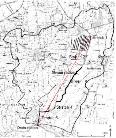
Figure 4.7 The Odder Bæk catchment with indications of stretches and lengths used for drift calculations.
Figur 4.7 Odder Bæk-oplandet med angivelse af strækninger og længder anvendt til drift-beregninger.
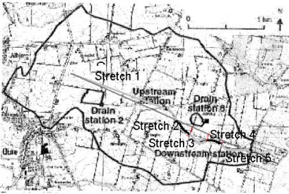
Figure 4.8 The Lillebæk catchment with indications of stretches and lengths used for drift calculations.
Figur 4.8 Lillebæk-oplandet med angivelse af strækninger og længder anvendt til drift-beregninger.
It is possible to specify width of buffer zones in the interface to the model. These values only overrule the existing buffer zones if the value is larger than the existing buffer zone.
For the pond scenarios, the logic applied for the calculations is different. Winddrift is calculated as if the ponds were square, that is 20 * 20 m² for Odder Bæk and approximately 15.8 * 15.8 m² for Lillebæk. The exposed length is therefore 20 and 15.8 m respectively. The calculation of drift is integrated over the width of the pond.
4.3 Dry deposition
The simulation of dry deposition takes place with a model “outside” the MIKE SHE/MIKE 11 model system. The model used is described in Asman et al. (2003) and in the technical documentation (Styczen et al., 2004c). An example of an input file for calculation is shown in Table 4.3. In the table is described how the parameters used are generated. The values either stem from the user interface, are pre-calculated such as information about water body cross sections and width of upland and organic matter content of the soil, or are generated from the MIKE 11 or MIKE SHE water simulations.
With respect to dry deposition, the outstanding question was the size of the agricultural area upwind of the pond. It was decided that it was not reasonable to determine the length of the upwind area based on the hydrological catchment to the pond. Also, it was unreasonable to let the upwind area depend on where in the catchment the site for the pond was selected. It was finally chosen to use the same upwind length for the ponds as has been used for the stream in the respective area.
Due to the fact that the module requires certain values from the water simulations of MIKE 11 and MIKE SHE, the model is executed after the water simulations are carried out and before the solute transport is calculated. In this way, the necessary stream flow parameters can be extracted from the result files and used for the simulation of dry deposition.
Table 4.3 Overview of input to the dry deposition model and the sources of information used for parameterisation.
Tabel 4.3 Oversigt over input til tørdepositionsmodellen, og kilderne til den anvendte parameterisering.
4.4 Calculation of effective pesticide dose on the soil
The input to the soil surface depends on the sprayed dosage and the processes described in 4.1 – 4.3. The pesticide dosage specified in the input file is modified in the following manner:
- If no plants are present on the field, the amount of drift is calculated, and the amounts of dry deposition on the stream and buffer zones are calculated. The total amount is deducted from the total sprayed amount, and the result is divided by the sprayed area. This figure is the input to the unsaturated zone. Emission from and re-deposition to the soil surface is not taken into account.
- If plants are present, the emission of pesticide of relevance for dry deposition is expected to stem from the leaf surfaces. The dosage reaching the soil is therefore only regulated according to the deposition figures by Jensen and Spliid (2003) and for wind drift.
All parameters from the calibrated model relating to transport in the root zone are used directly in the scenario-models. These parameters are described in Styczen et al. (2004a).
4.5 Adsorption to macrophytes
The parameterisation of the sorption to macrophytes included two step. First a Kd value for the sorption to macrophytes was calculated on the basis of an empirical relationship between water solubility and Kd values for different macrophytes and pesticides (1) derived by Crum et al. (1999).
log(Kd) = 3.2 – 0.65 log(S), (1)
where
S denotes the water solubility (mg/l).
Furthermore, it was assumed that the ratio between the sorption and desorption rates is given by the Kd value and that sorption rate is compound and sorbant independent and therefore similar to the sorption rate estimated for the sorption experiments with stream and pond sediments.
The biomass of macrophytes in the stream scenario was estimated on the basis of information from the literature of the yearly succession in the biomass of macrophytes in Danish streams not covered by forest (Sand-Jensen and Lindegaard, 1996). To take the effect of forest cover into account the fraction of the streams covered by forest was therefore estimated by visual inspections along the streams as 0% for Odder Bæk and 50% for Lillebæk. It was then assumed that no macrophytes was present where the stream is covered by forest and the biomass shown on Figure 4.9 was thus multiplied with 0.5 for Lillebæk and 1 for Odder Bæk. The conversion from the unit of g m-2 shown on Figure 4.9 to the unit of g*m-3 used in the model thus assumed an average depth of 0.10 m for Lillebæk and 0.5 m for Odder Bæk respectively.
Figure 4.9 Macrophyte biomass in light open streams
Figur 4.9 Makrofyt-biomasse i lyseksponerede åbne vandløb.
According to the scenario definitions the ponds can be either phytoplankton or macrophyte dominated. These choices are based on a fundamental ecological classification of small Danish lakes, which is illustrated on Figure 4.10. It is the intention that the suite of scenarios together should reflect these classification. Hence the scenarios of macrophyte dominated ponds are supposed to mimic ponds with high density of submerged macrophytes classified as oligortrophic to mesotrophic on Figure 4.10, whereas the phytoplankton dominated scenario is supposed to mimic hypereutrophic conditions. The most oligotrophic conditions are generally found in lakes in sandy catchments and it was therefore decided to let the pond of Odder Bæk be an image of this. Hence the concentration of macrophytes in the pond of Odder Bæk was set to 50 g/m³ corresponding to the biomass of macrophytes to the very left at Figure 4.10.
Figure 4.10 General changes in the balance between phytoplankton, submerged vegetation and floating vegetation and reed swamp along eutrophication gradient.
Figur 4.10 Generelle ændringer i balancen mellem fytoplankton, vanddækket vegetation og flydende vegetation og rørsump som funktion af eutrofiering.
The lakes of the eastern part of Denmark is naturally more eutrophicated than the lakes of the western part. To take this into account the concentration of macrophytes in the macrophyte dominated pond of Lillebæk was set to 700 g/m² corresponding to a biomass of up to 200 to 700 g/m² reported for dense populations of submerged macrophytes in Danish lakes (Jensen og Lindegaard, 1996). Hence, the dense macrophyte populations of the ponds of Lillebæk might reflect both natural and anthropogenic eutrophication.
4.6 Adsorption to suspended matter
Even for active substances with a high Kd for adsorption to suspended matter most of the active substance is found as dissolved substance in the water column. For instance, for the active substance pendimetahlin, with a Kd value as high as 640 l kg-1 only 6 % of the mass will be sorbed at equilibrium at a particle concentration as high as 100 mg l-1. Sorption to suspended matter in the water column was therefore not considered as important in the model. The particle concentration in streams and ponds was therefore given by the amount of particles transported from the catchment into the streams and ponds through macropore flow. Hence, no attempts to adjust for the production of particles in the ponds and streams were made.
4.7 Sediment in streams and ponds
In the streams an upper sediment layer of a thickness of about 2 cm is built up during the summer season and subsequently removed during flood events in the winter season (Iversen et al., 2003). Compared to the lower more crude sediment the content of organic matter in this upper sediment layer is high. Since the extent of sorption of pesticide to sediment particles mainly is related to the content of organic matter only the upper few cm of newly settled sediment is supposed to be of significance for the fate and transport of pesticides in the streams. The thickness of the sediment was therefore set to 2 cm. The porosity of the sediments and the content of organic matter, which is needed for description of the biodegradation, the diffusion and the sorption were reported by Helweg et al. (2003) and appear from Table 4.4.
Table 4.4 Porosity and organic content of the sediment of the different scenaria
| Scenario | Loss of ignition (g/kg d.w.) |
Porosity |
| Lillebæk pond – macrophyt dom. | 82 | 0.75 |
| Lillebæk pond – phytoplan. dom. | 600 | 0.95 |
| Lillebæk stream | 25 | 0.75 |
| Odder Bæk pond – macrophyt dom. | 82 | 0.75 |
| Odder Bæk pond – phytoplan. dom. | 600 | 0.95 |
| Odder Bæk stream | 197 | 0.75 |
For the macrophyte dominated pond the porosity of the sediments and the content of organic matter was set equal to the measurements from the artificial ponds at NERI in Roskilde. The sediment of the phytoplankton dominated ponds is supposed to be very high in organic content, since the scenario is supposed to mimic hypereutrophic ponds with a high production of phytoplankton, which is sedimentating in the pond. The content of organic matter was therefore set to 60% corresponding to the highest loss of ignitions measured for 15 Danish lakes with a high content of organic matter in the sediments. Furthermore the porosity was set to 0.95 reflecting the high water content of sediments rich in organic matter (Miljøstyrelsen 1991).
As a consequence of the high content of organic matter long periods with anoxic conditions in the sediment might frequently be found in such ponds. When the biodegradation was parameterized for the phytoplankton dominated ponds it was therefore assumed that the biodegradation is anaerobic.
We are aware of that the attempt to summarize the ecological conditions in streams and ponds in terms of the selected scenario is a crude generalisation of the complex ecological condition of such systems. This consquences of this is discussed further in Section 7.1.
Version 1.0 Maj 2004, © Danish Environmental Protection Agency