Evaluation of Pesticide Scenarios for the Registration Procedure
Appendix C Calibration of PLAP Models
1.1 Calibration of PLAP Scenarios
The 1-dimensional MACRO model vs. 5.1 (Larsbo and Jarvis, 2003) is applied to the five PLAP sites Tylstrup, Jyndevad, Silstrup, Estrup, and Faardrup covering the soil profile to a depth of 5 m b.g.s., always including the groundwater table. The model is calibrated against water saturation measured in suction cells, depth to groundwater table measured in piezometers, drainage runoff and bromide concentration in water sampled from either suction cups or drainage system during the full monitoring period May 1999 – June 2004. A typical horizontal and vertical lay-out of monitoring devices at a tile-drained site is shown in Figures C1 and C2.
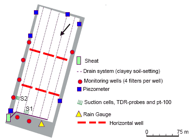
Figure C1. A typical horizontal lay-out of monitoring devices at a tile-drained PLAP site.
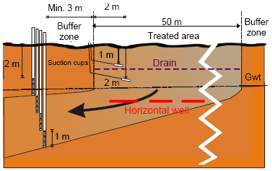
Figure C2. A typical vertical lay-out of monitoring devices at a tile-drained PLAP site.
At each site there is spatial heterogeneity. Therefore, the fact that some measurements can be regarded as point measurements and others as integrating over an area has caused the data used in the calibration to be weighted differently. Most emphasis in the calibration has been given to the integrated measurements. They are the groundwater table, measured yearly drainage, and the accumulated bromide leaching in drains.
At the two sand locations there are no integrated measurements of bromide. Instead the bromide transport is calibrated with even emphasis on breakthrough curves at 1 and 2 m b.g.s. from both tracer experiments.
An overview of calibration results is given in Table C1. More detailed information on collected data and the calibration results at each site can be found in the following sections.
Table C1. Overview of calibration results for PLAP scenarios.
| Calibration results | Location | ||||
| Data-type | Tylstrup | Jyndevad | Silstrup | Estrup | Faardrup |
| Flow related: | |||||
| - Depth to groundwater table (GWT) | Level of GWT: Fluctuations: Amplitude less well described |
Level of GWT: Fluctuations: SIM ~ OBS |
Level of GWT: Fluctuations: Initial rise in autumn too late |
Level of GWT: Fluctuations: |
Level of GWT: Fluctuations: |
| - Soil Water Content | |||||
| 0.25 m b.g.s. (SW25) | Level of SW25: SIM often a bit higher than OBS Fluctuations: |
Level of SW25: SIM often a bit higher than OBS Fluctuations: |
Level of SW25: Fluctuations: |
Level of SW25: SIM ~ OBS Fluctuations: Min. OBS not well described |
Level of SW25: SIM ~ OBS Fluctuations: |
| 0.60 m b.g.s. (SW60) | Level of SW60: SIM often a bit higher than OBS Fluctuations: |
Level of SW60: SIM often a bit higher than OBS Fluctuations: |
Level of SW60: Fluctuations: SIM a bit earlier than OBS |
- | Level of SW60: Fluctuations: SIM shape OBS shape |
| 1.10 m b.g.s. (SW110) | Level of SW110: Fluctuations: Min. OBS less well described |
Level of SW110: SIM much lower than OBS Fluctuations: |
Level of SW110: SIM ~ OBS excluding TDR-OBS-errors Fluctuations: Min. OBS less well described excluding TDR-OBS-errors |
- TDR-OBS-errors |
Level of SW110: Fluctuations: |
| - Drainage | - | - | SIM ~ OBS | SIM ~ OBS | SIM ~ OBS |
| Transport related: | |||||
| - Bromide - suction cells | |||||
| 1 m b.g.s. | 1. Peak 2. Peak Breakthrough time: SIM 2 month earlier than OBS Shape/Size: SIM narrower than OBS |
1. Peak 2. Peak Breakthrough time: SIM 4 month too late compared to OBS Shape/Size: SIM narrower than OBS |
Peak Breakthrough time: Shape/Size: SIM amount < OBS amount in June and July 2000 |
Peak Breakthrough time: Shape/Size: SIM ~ OBS |
Peak Breakthrough time: Shape/Size: SIM ~ OBS Maybe SIM amount > OBS amount |
| 2 m b.g.s. | 1. Peak 2. Peak Breakthrough time: Shape/Size: |
1. Peak 2. Peak Breakthrough time: Shape/Size: |
- (SIM ~ OBS Temporarily below GWT- Not used in the calibration procedure) |
- ( SIM ~ OBS Temporarily below GWT- Not used in the calibration procedure) |
- (SIM ~ OBS Temporarily below GWT- Not used in the calibration procedure) |
| - Bromide – monitoring wells at app. 3 m b.g.s. | SIM ~ OBS (GWT 3-4m b.g.s.) |
SIM ~ OBS (GWT 1-3m b.g.s.) |
SIM ~ OBS (GWT 1-3m b.g.s.) |
SIM ~ OBS (GWT 0-4m b.g.s.) |
SIM ~ OBS (GWT 1-3m b.g.s.) |
| - Acc. bromide leaching in drains | - | - | Breakthrough time: () Shape/Size: SIM ~ OBS excluding Jan- May 2004 |
Breakthrough time: Shape/Size: SIM ~ OBS excluding Jan- May 2004 |
Breakthrough time: Shape/Size: SIM ~ OBS since climate series is obtained from station at bit away |
1.1.1 Data
The extensive amount of data collected within the PLAP programme form the basis of the calibration of the scenarios. The following provides an overview of selected data, while detailed information on data acquisition and model set-up are provided by Kjær et al. (2005). For further information on site characterization and monitoring design see Lindhardt et al. (2001).
1.1.1.1 Climate
An automated monitoring system has been installed at each site for measurement of precipitation and barometric pressure. The annual precipitation measured by DIAS and corrected to the soil surface according to the method of Allerup and Madsen (1979) is shown for each site in Table C2.
Table C2. Annual precipitation (mm/year) and potential evapotranspiration (mm/year) at the five sites for the monitoring period.
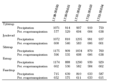
The potential evapotranspiration has been calculated at DIAS using a modified Makkink equation (Aslyng and Hansen, 1982). The potential evapotranspiration is defined as the evapotranspiration from well-growing short grass adequately supplied with water. The annual potential evapotranspiration at each site is shown in Table 1, and more detailed information on climate data is given in Kjær et al. (2005).
1.1.1.2 Soil
Geological and pedological investigations have been carried out at all sites. Two to three soil profiles have been excavated and described and soil samples have been collected and analyzed. An overview of the soil type at the five sites is given in Table C3.
Table C3. Soil types for the five sites.
| Site | Tylstrup | Jyndevad | Silstrup | Estrup | Faardrup |
| Soil type | Fine sand | Coarse sand | Clayey till | Clayey till | Clayey till |
| Deposited by | Saltwater | Melt water | Glacier | Glacier | Glacier |
For more results on geological and pedological investigations see Lindhardt et al. (2001).
1.1.1.3 Soil Hydrology and Organic Matter
Soil cores (100 cm³ and 6,280 cm³) for the measurement of hydrological properties (soil water characteristics and hydraulic conductivity) have been sampled at three levels corresponding to the A, B and C horizons in the two to three excavated soil profiles at the sites.
The soil water characteristics of the nine small cores (100 cm³) from each horizon are shown together with bulk density, porosity and organic matter in Tables C4 – C8. Measurements of saturated hydraulic conductivity and air permeability using small (100 cm³) or large (6,280 cm³) soil samples at the sites are shown in Figures C3 – C7 corresponding to the three horizons. Additional information on monitoring design and hydraulic data can be found in Lindhardt et al. (2001).
Table C4. Soil water characteristics at Tylstrup determined on the small soil cores, pF = log10(-h). 1) Assuming a particle density of 2.65 g cm-3, 2) Not measured, and 3) Mid-point of the soil core. 4) OM: Organic matter in horizon, OM = 1.72 x TOC. Analysed by DIAS. (Lindhardt et al., 2001)
| Profile no. | Horizon | Depth³ [cm b.g.s.] |
Water content at pF values [cm³ cm-3] |
Bulk density [g cm-3] |
Porosity1 [cm³cm-3] |
OM 4 [%] |
||||||
| 1.0 | 1.2 | 1.7 | 2.0 | 2.2 | 3.0 | 4.2 | ||||||
| 1 (3087) | Ap | 15 | 0.44 | 0.43 | 0.41 | 0.33 | 0.28 | 0.15 | 0.04 | 1.33 | 0.50 | 2.7 |
| Bv | 55 | 0.48 | 0.47 | 0.40 | 0.23 | 0.18 | 0.10 | 0.05 | 1.31 | 0.50 | 2.0 | |
| BC | 80 | 0.45 | 0.44 | 0.41 | 0.24 | 0.16 | 0.07 | 0.01 | 1.40 | 0.47 | 0.3 | |
| 2 (West) | Ap | 15 | 0.42 | 0.41 | 0.41 | 0.36 | 0.28 | 0.16 | 2) | 1.45 | 0.45 | 2) |
| Bh | 60 | 0.44 | 0.42 | 0.33 | 0.19 | 0.15 | 0.10 | 2) | 1.39 | 0.48 | 2) | |
| C | 100 | 0.40 | 0.38 | 0.31 | 0.16 | 0.11 | 0.06 | 2) | 1.51 | 0.43 | 2) | |
| 3 (3088) | Ap1 | 15 | 0.41 | 0.41 | 0.38 | 0.33 | 0.27 | 0.15 | 0.05 | 1.45 | 0.45 | 2.7 |
| Ap2 | 50 | 0.39 | 0.38 | 0.31 | 0.18 | 0.14 | 0.08 | 0.03 | 1.50 | 0.44 | 1.4 | |
| C | 100 | 0.40 | 0.39 | 0.37 | 0.21 | 0.12 | 0.05 | 0.01 | 1.51 | 0.43 | 0.2 | |
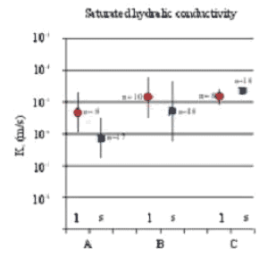
Figure C3. Measured at Tylstrup: Saturated hydraulic conductivity (Ks) measured on large (6,280 cm³) samples (![]() ) and small (100 cm³) samples (
) and small (100 cm³) samples (![]() ). (Lindhardt et al., 2001)
). (Lindhardt et al., 2001)
Table C5. Soil water characteristics at Jyndevad determined on the small soil cores, pF = log10(-h). 1) Assuming a particle density of 2.65 g cm-3, 2) Not measured, and 3) mid-point of the soil core. 4) OM: Organic matter in horizon, OM = 1.72 x TOC. Analysed by DIAS. (Lindhardt et al., 2001)
| Profile no. | Horizon | Depth³ [cm b.g.s.] |
Water content at pF values [cm³ cm-3] |
Bulk density [g cm-3] |
Porosity1 [cm³ cm-3] | OM 4 [%] |
||||||
| 1.0 | 1.2 | 1.7 | 2.0 | 2.2 | 3.0 | 4.2 | ||||||
| 1 (3092) | Ap | 15 | 0.41 | 0.40 | 0.23 | 0.19 | 0.17 | 0.12 | 0.04 | 1.37 | 0.48 | 2.3 |
| Bhs/Bs | 40 | 0.35 | 0.33 | 0.15 | 0.11 | 0.10 | 0.07 | 0.01 | 1.49 | 0.44 | 1.3/0.3 | |
| BC | 115 | 0.34 | 0.32 | 0.10 | 0.06 | 0.06 | 0.04 | 0.01 | 1.52 | 0.43 | 0.1 el. 0.3 | |
| 2 (3091) | Ap | 15 | 0.40 | 0.39 | 0.28 | 0.22 | 0.20 | 0.13 | 0.05 | 1.42 | 0.47 | 3.4 |
| Bhs/Bs | 40 | 0.39 | 0.36 | 0.20 | 0.15 | 0.14 | 0.10 | 0.03 | 1.38 | 0.48 | 1.9/0.5 | |
| C | 130 | 0.34 | 0.28 | 0.09 | 0.07 | 0.06 | 0.05 | 0.01 | 1.48 | 0.44 | 0.1 | |
| 3(North) | Ap | 15 | 0.39 | 0.38 | 0.22 | 0.17 | 0.16 | 0.11 | 0.03 | 1.43 | 0.46 | 2) |
| Bhs | 40 | 0.37 | 0.35 | 0.10 | 0.07 | 0.07 | 0.05 | 0.03 | 1.47 | 0.44 | 2) | |
| C | 110 | 0.34 | 0.32 | 0.09 | 0.06 | 0.05 | 0.04 | 0.01 | 1.50 | 0.43 | 2) | |
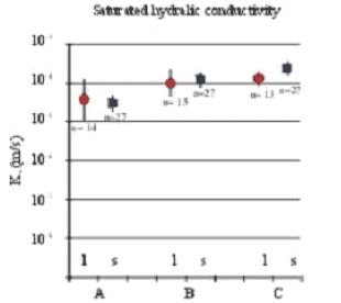
Figure C4. Measured at Jyndevad: Saturated hydraulic conductivity (Ks) measured on large (6,280 cm³) samples (![]() ) and small (100 cm³) samples (
) and small (100 cm³) samples (![]() ). (Lindhardt et al., 2001)
). (Lindhardt et al., 2001)
Table C6. Soil water characteristics at Silstrup determined on the small soil cores, pF = log10(-h). 1) Assuming a particle density of 2.65 g cm-3, 2) Not measured, and 3) mid-point of the soil core. 4) OM: Organic matter in horizon, OM = 1.72 x TOC. Analysed by DIAS. (Lindhardt et al., 2001)
| Profile no. |
Horizon | Depth³ [cm b.g.s.] |
Water content at pF values [cm³ cm-3] |
Bulk density [g cm-3] |
Porosity1 [cm³ cm-3] |
OM 4 [%] |
||||||
| 1.0 | 1.2 | 1.7 | 2.0 | 2.2 | 3.0 | 4.2 | ||||||
| 1 (3093) | Ap | 15 | 0.39 | 0.38 | 0.36 | 0.35 | 0.34 | 0.28 | 0.13 | 1.42 | 0.46 | 3.4 |
| Bv | 40 | 0.35 | 0.35 | 0.32 | 0.31 | 0.30 | 0.25 | 0.16 | 1.62 | 0.39 | 0.5 | |
| BC(g) | 150 | 0.30 | 0.30 | 0.29 | 0.28 | 0.28 | 0.26 | 0.16 | 1.77 | 0.33 | 0.2 | |
| 2 (3094) | Ap | 15 | 0.37 | 0.36 | 0.35 | 0.34 | 0.34 | 0.29 | 0.14 | 1.54 | 0.42 | 2.8 |
| Bv | 40 | 0.36 | 0.36 | 0.35 | 0.34 | 0.33 | 0.29 | 0.15 | 1.59 | 0.40 | 0.5 | |
| Cc | 90 | 0.31 | 0.30 | 0.29 | 0.29 | 0.28 | 0.26 | 0.12 | 1.73 | 0.35 | 2) | |
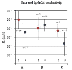
Figure C5. Measured at Silstrup: Saturated hydraulic conductivity (Ks) measured on large (6,280 cm³) samples (![]() ) and small (100 cm³) samples (
) and small (100 cm³) samples (![]() ). (Lindhardt et al., 2001)
). (Lindhardt et al., 2001)
Table C7. Soil water characteristics at Estrup determined on the small soil cores, pF = log10(-h). 1) Assuming a particle density of 2.65 g cm-3, 2) Not measured, and 3) mid-point of the soil core. 4) OM: Organic matter in horizon, OM = 1.72 x TOC. Analysed by DIAS. (Lindhardt et al., 2001)
| Profile no. | Horizon | Depth³ [cm b.g.s.] |
Water content at pF values [cm³ cm-3] |
Bulk density [g cm-3] |
Porosity1 [cm³ cm-3] |
OM 4 [%] |
||||||
| 1.0 | 1.2 | 1.7 | 2.0 | 2.2 | 3.0 | 4.2 | ||||||
| 1 (3099) | Ap | 15 | 0.35 | 0.34 | 0.33 | 0.31 | 0.30 | 0.24 | 0.09 | 1.56 | 0.41 | 2.7 |
| Bt(g) 2 | 36 | 0.33 | 0.32 | 0.31 | 0.30 | 0.29 | 0.26 | 0.20 | 1.73 | 0.35 | 0.2 | |
| Cc 2 | 122 | 0.37 | 0.37 | 0.36 | 0.36 | 0.35 | 0.33 | 0.22 | 1.78 | 0.33 | 0.5 | |
| 2 (3098) | Ap | 15 | 0.37 | 0.36 | 0.34 | 0.33 | 0.33 | 0.27 | 0.13 | 1.56 | 0.41 | 4.2 |
| BE(g) 2 | 50 | 0.38 | 0.38 | 0.37 | 0.37 | 0.37 | 0.33 | 0.06 | 1.67 | 0.37 | 0.5 | |
| 3Cg 2 | 122 | 0.45 | 0.45 | 0.45 | 0.44 | 0.44 | 0.41 | 0.02 | 1.59 | 0.40 | 0.1 | |
| 3 (3100) | Ap | 15 | 0.42 | 0.41 | 0.39 | 0.38 | 0.38 | 0.31 | 0.10 | 1.42 | 0.46 | 5.5 |
| Bhs 2 | 38 | 0.33 | 0.32 | 0.29 | 0.27 | 0.27 | 0.23 | 0.04 | 1.69 | 0.36 | 0.8 | |
| 2C 2 | 120 | 0.42 | 0.42 | 0.42 | 0.41 | 0.40 | 0.37 | 0.31 | 1.55 | 0.42 | 2) | |
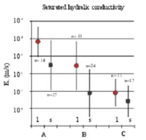
Figure C6. Measured at Estrup: saturated hydraulic conductivity (Ks) measured on large (6,280 cm3) samples (![]() ) and small (100 cm3) samples (
) and small (100 cm3) samples (![]() ). (Lindhardt et al., 2001)
). (Lindhardt et al., 2001)
Table C8. Soil water characteristics at Faardrup determined on the small soil cores, pF = log10(-h). 1) Assuming a particle density of 2.65 g cm-3, 2) Not measured, and 3) mid-point of the soil core. 4) OM: Organic matter in horizon, OM = 1.72 x TOC. Analysed by DIAS. (Lindhardt et al., 2001)
Profile no. |
Horizon | Depth³ [cm b.g.s.] |
Water content at pF values [cm³ cm-3] |
Bulk density [g cm-3] |
Porosity1 [cm3 cm-3] |
OM 4 [%] |
||||||
| 1.0 | 1.2 | 1.7 | 2.0 | 2.2 | 3.0 | 4.2 | ||||||
| 1 (West) | Ap | 15 | 0.37 | 0.36 | 0.32 | 0.30 | 0.28 | 0.21 | 0.08 | 1.42 | 0.46 | 2) |
| Bvt | 75 | 0.32 | 0.31 | 0.28 | 0.26 | 0.25 | 0.20 | 0.13 | 1.60 | 0.40 | 2) | |
| Cc(g) | 120 | 0.27 | 0.27 | 0.25 | 0.23 | 0.23 | 0.21 | 0.10 | 1.84 | 0.31 | 2) | |
| 2(3090) | Ap | 15 | 0.32 | 0.31 | 0.29 | 0.28 | 0.27 | 0.22 | 0.09 | 1.73 | 0.35 | 2.6 |
| Bv | 80 | 0.32 | 0.31 | 0.29 | 0.27 | 0.26 | 0.22 | 0.10 | 1.70 | 0.36 | 0.4 | |
| Cc(g) | 130 | 0.29 | 0.28 | 0.27 | 0.26 | 0.25 | 0.23 | 0.09 | 1.78 | 0.33 | 0.2 - 0.4 | |
| 3(3089) | Ap | 15 | 0.38 | 0.37 | 0.33 | 0.32 | 0.30 | 0.24 | 0.08 | 1.52 | 0.43 | 2.4 |
| Bvt(g) | 80 | 0.32 | 0.30 | 0.27 | 0.25 | 0.24 | 0.20 | 0.15 | 1.70 | 0.36 | 0.2 | |
| Cc(g) | 130 | 0.29 | 0.28 | 0.26 | 0.25 | 0.24 | 0.22 | 0.10 | 1.83 | 0.31 | 0.1 | |
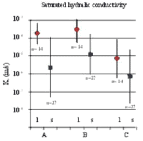
Figure C7. Measured at Faardrup: Saturated hydraulic conductivity (Ks) measured on large (6,280 cm³) samples (![]() ) and small (100 cm³) samples (
) and small (100 cm³) samples (![]() ). (Lindhardt et al., 2001)
). (Lindhardt et al., 2001)
1.1.1.4 Crop
The crops grown at the five sites during the full monitoring period are shown in Table C9.
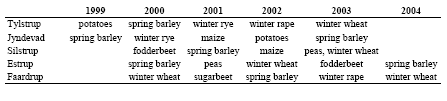
Table C9. Crops grown at the five sites during the monitoring period.
1.1.1.5 Bromide Application
Bromide in a dose of 30 kg/ha has been applied to the five sites at the dates shown in Table C10.
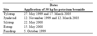
Table C10. Dates of bromide application.
1.1.2 Calibration of Tylstrup Model
The model for the Tylstrup site has been calibrated for the whole period to the observed groundwater table measured in the piezometers located in the buffer zone, to time series of soil water content measured at three different depths (25, 60 and 110 cm b.g.s.) from the two profiles S1 and S2 (see Figure C8) and to the bromide concentration measured in the suction cups located 1 and 2 m b.g.s. The model is evaluated with respect to monitoring measurements of bromide below 3 m b.g.s. Data acquisition and model set-up are described in Kjær et al. (2005) appendix 4. The main calibration parameters were the empirical parameter, BGRAD, which regulates the boundary flow, the “boundary” pressure head (CTEN), its corresponding water content (XMPOR), the hydraulic conductivity (KSM), the dispersivity (DV), the mixing depth (ZMIX) and the effective diffusion path length (ASCALE), which controls the exchange of water and solute between the two flow domains (see Kjær et al. (2005) appendix 4 for details). In addition the solute concentration factor (FSTAR) is calibrated. It accounts for crop uptake of solute in the transpiration stream.
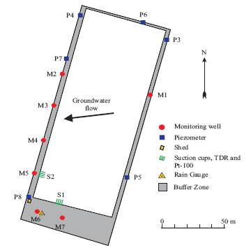
Figure C8. Overview of the Tylstrup test site. The innermost white area indicates the cultivated land, while the grey area indicates the surrounding buffer zone. The positions of the various installations are indicated, as is the direction of groundwater flow (by an arrow). (Kjær et al., 2005)
1.1.3 Soil Water Dynamics and Water Balances
The model simulations are generally consistent with the observed data, thus indicating a good model description of the overall soil water dynamics in the unsaturated zone. The model provides a good simulation of the measured dynamics in the groundwater table (Figure C9-B) but the amplitude of the fluctuations is less well described. The overall trends in soil water content are modelled successfully, with the model capturing soil water dynamics at all depths (Figure C9-C to E). The simulated soil water content in 0.25 and 0.6 m b.g.s. is a little above observed values.
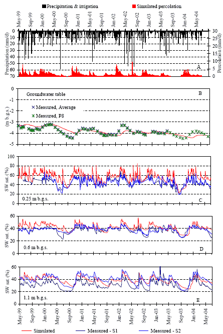
Figure C9. Soil water dynamics at Tylstrup: Measured precipitation, irrigation and simulated percolation 1 m b.g.s. (A), simulated and measured groundwater level (B), and simulated and measured soil water saturation (SW sat.) at three different soil depths (C, D and E). The measured data in B derive from piezometers located in the buffer zone. The measured data in C, D and E derive from TDR probes installed at S1 and S2 (Figure C8).
The resulting annual water balance for Tylstrup is shown for each monitoring period (July–June) in Table C11. For additional information about the water balance in the monitoring period see Kjær et al. (2005).
Table C11. Annual water balance for Tylstrup (mm yr-1). Precipitation is corrected to the soil surface according to the method of Allerup and Madsen (1979). 1) Accumulated for a two-month period, 2) Normal values based on time series for 1961–1990, and 3) Groundwater recharge is calculated as precipitation + irrigation - actual evapotranspiration.
| Period | Normal precipitation 2) |
Precipitation | Irrigation | Actual Evapo-transpiration |
Groundwater recharge 3) |
| 1.5.99–30.6.991) | 120 | 269 | 0 | 112 | 156 |
| 1.7.99–30.6.00 | 773 | 1073 | 33 | 498 | 608 |
| 1.7.00–30.6.01 | 773 | 914 | 75 | 487 | 502 |
| 1.7.01–30.6.02 | 773 | 906 | 80 | 570 | 416 |
| 1.7.02–30.6.03 | 773 | 918 | 23 | 502 | 439 |
| 1.7.03–30.6.04 | 773 | 759 | 0 | 472 | 286 |
1.1.4 Bromide Leaching
Bromide has been applied twice at Tylstrup. In the unsaturated zone the first breakthrough of bromide (deriving from the first application in 1999) is well described by MACRO 5.1 (Figure C10). The dynamics of the second breakthrough of bromide (deriving from the bromide applied in 2003) is less well described by the model (Figure C10). The breakthrough 1 m b.g.s. is simulated two months too early, the concentration increases too rapidly, and the peak is too high compared to the measured profile. At 2 m b.g.s. the simulated concentration decreases too slowly, resulting in a concentration profile that is much wider than the measured profile. Reducing the discrepancies between measured and simulated breakthrough curves in the suction cups was tried by the use of the inverse programme SUFI (Abbaspour et al., 1997) but this was not successful.
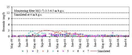
Bromide has been measured below the groundwater table in monitoring wells. Because MACRO is a 1-dimensional model it is not correct to calibrate the model to concentrations below the groundwater table. Instead simulated bromide leaching below the groundwater table is evaluated against occurrence of measured bromide at same depths. Measured bromide concentration in the groundwater at 3.5 – 4.5 m b.g.s. in seven wells and simulated bromide concentration at 4 m b.g.s. are shown in Figure C11. The simulated leaching is in agreement with the measured occurrence of bromide.
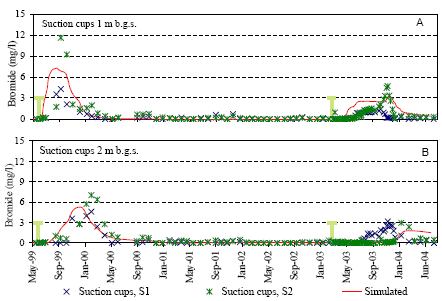
Figure C10. Simulated and measured bromide concentration in the unsaturated zone at Tylstrup: Simulated and measured bromide concentrations at 1 m b.g.s. (A) and 2 m b.g.s. (B). The measured data in A and B derive from suction cups installed 1 m b.g.s. and 2 m b.g.s. at locations S1 and S2 indicated in Figure C8. The green vertical lines indicate the dates of bromide application.
Figure C11. Measured bromide concentration in the groundwater at 3.5 – 4.5 m b.g.s, and simulated bromide concentration at 4 m b.g.s. at Tylstrup. The measured data derive from monitoring wells M1–M7 indicated in Figure C8.
1.1.5 Calibration of Jyndevad Model
The model for the Jyndevad site has been calibrated for the whole monitoring period to the observed groundwater table measured in the piezometers located in the buffer zone, to time series of soil water content measured at three different depths (25, 60 and 110 cm b.g.s.) from the two profiles S1 and S2 (see Figure C12), and to the bromide concentration measured in the suction cups located 1 and 2 m b.g.s. The model is evaluated with respect to monitoring measurements of bromide below 3 m b.g.s. Data acquisition and model set-up are described in Kjær et al. (2005) appendix 4. The main calibration parameters were the empirical parameter BGRAD, which regulates the boundary flow, the “boundary” pressure head (CTEN), its corresponding water content (XMPOR), the hydraulic conductivity (KSM), the dispersivity (DV), the mixing depth (ZMIX) and the effective diffusion path length (ASCALE), which controls the exchange of water and solute between the two flow domains (see Kjær et al. (2005) appendix 4 for details). In addition the solute concentration factor (FSTAR) is calibrated. It accounts for crop uptake of solute in the transpiration stream.
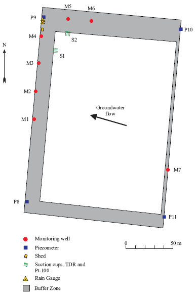
Figure C12. Overview of the Jyndevad test site. The innermost white area indicates the cultivated land, while the grey area indicates the surrounding buffer zone. The positions of the various installations are indicated, as is the direction of groundwater flow (by an arrow). (Kjær et al., 2005).
1.1.6 Soil Water Dynamics and Water Balances
The model simulations are generally consistent with the observed data, thus indicating a good model description of the overall soil water dynamics in the unsaturated zone (Figure C13). The dynamics of the simulated groundwater table is well described. However, as noted in Kjær et al. (2004), the model has some difficulty in capturing the degree of soil water saturation 1.1 m b.g.s. (Figure C13-E).
The resulting annual water balance for Jyndevad for the five monitoring periods (July–June) is shown in Table C12. For additional information about the water balance in the monitoring period see Kjær et al. (2005).
Table C12. Annual water balance for Jyndevad (mm yr-1). Precipitation is corrected to the soil surface according to the method of Allerup and Madsen (1979). 1) Normal values based on time series for 1961–1990, and 2) Groundwater recharge is calculated as precipitation + irrigation - actual evapotranspiration
| Period | Normal precipitation 1) |
Precipitation | Irrigation | Actual Evapo-transpiration |
Groundwater recharge 2) |
| 1.7.99–30.6.00 | 995 | 1073 | 29 | 500 | 602 |
| 1.7.00–30.6.01 | 995 | 810 | 0 | 461 | 349 |
| 1.7.01–30.6.02 | 995 | 1204 | 81 | 545 | 740 |
| 1.7.02–30.6.03 | 995 | 991 | 51 | 415 | 627 |
| 1.7.03–30.6.04 | 995 | 936 | 27 | 429 | 534 |
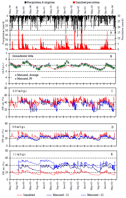
Figure C13. Soil water dynamics at Jyndevad: Measured precipitation, irrigation and simulated percolation 1 m b.g.s. (A), simulated and measured groundwater level (B), and simulated and measured soil water saturation (SW sat.) at three different soil depths (C, D and E). The measured data in B derive from piezometers located in the buffer zone. The measured data in C, D and E derive from TDR probes installed at S1 and S2 (see Figure C12).
1.1.7 Bromide Leaching
Bromide has been applied twice at Jyndevad. In the unsaturated zone the first breakthrough of bromide (deriving from the first application in 1999) is well described by MACRO 5.1 (Figure C14). The dynamics of the second breakthrough of bromide (deriving from the bromide applied in 2003) is well described by the model in 2 m b.g.s. but less well described in 1 m b.g.s. (Figure C14). At 1 m b.g.s. the second breakthrough is simulated four months too late, and the concentration profile is much narrower than the measured profile. Reducing the discrepancies between measured and simulated breakthrough curves in the suction cups was tried by the use of the inverse programme SUFI (Abbaspour et al., 1997) but this was not successful.
Bromide has been measured below the groundwater table in monitoring wells. Because MACRO is a 1-dimensional model it is not correct to calibrate the model to concentrations below the groundwater table. Instead simulated bromide leaching below the groundwater table is evaluated against occurrence of measured bromide at same depths. Measured bromide concentration in the groundwater at 2.5 – 3.5 m b.g.s. in seven wells and simulated bromide concentration at 3 m b.g.s. are shown in Figure C15. The simulated leaching is in agreement with the measured occurrence of bromide.
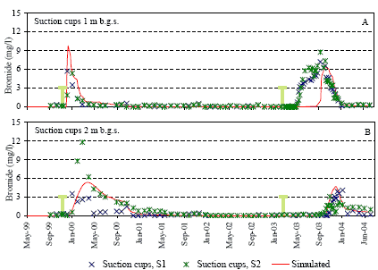
Figure C14. Simulated and measured bromide concentration in the unsaturated zone at Jyndevad: Simulated and measured bromide concentrations at 1 m b.g.s. (A) and 2 m b.g.s. (B). The measured data in A and B derive from suction cups installed 1 m b.g.s. and 2 m b.g.s. at locations S1 and S2 indicated in Figure C12. The green vertical lines indicate the dates of bromide application.
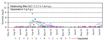
Figure C15. Measured bromide concentration in the groundwater at 2.5 – 3.5 m b.g.s, and simulated bromide concentration at 3 m b.g.s. at Jyndevad. The measured data derive from monitoring wells M1–M7 indicated in Figure C12.
1.1.8 Calibration of Silstrup Model
The model for the Silstrup site is calibrated for the whole monitoring period to the observed groundwater table measured in the piezometers located in the buffer zone, to time series of soil water content measured at three depths (25, 60 and 110 cm b.g.s.) from the two profiles S1 and S2 (see Figure C16), to the measured drainage flow, to the bromide concentration measured in the suction cups located 1 and 2 m b.g.s, and to measured bromide leaching in drains. The model is evaluated with respect to monitoring measurements of bromide below 3 m b.g.s. Data acquisition and model set-up are described in Kjær et al. (2005) appendix 4. The main calibration parameters were the empirical parameter BGRAD, which regulates the boundary flow, the “boundary” pressure head (CTEN), its corresponding water content (XMPOR), the hydraulic conductivity (KSM) and the effective diffusion path length (ASCALE), which controls the exchange of water and solute between the two flow domains (see Kjær et al. (2005) appendix 4 for details). In addition the solute concentration factor (FSTAR) is calibrated. It accounts for crop uptake of solute in the transpiration stream.
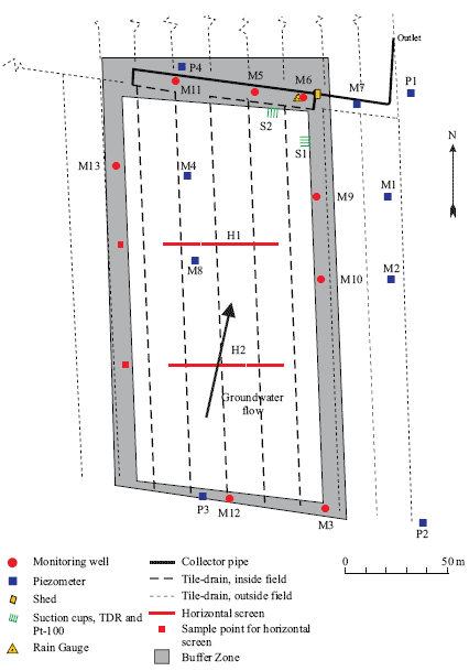
Figure C16. Overview of the Silstrup site. The innermost white area indicates the cultivated land, while the grey area indicates the surrounding buffer zone. The positions of the various installations are indicated, as is the direction of groundwater flow (by an arrow). (Kjær et al., 2005).
1.1.9 Soil Water Dynamics and Water Balances
The model simulations are generally consistent with the observed data, thus indicating a good model description of the overall soil water dynamics in the unsaturated zone (Figure C17). A closer study of measured groundwater table in the different piezometers show that it varies significantly, especially between the upstream (P2 and P3, see Figure C16) and downstream (P1 and P4) piezometers, as shown in Figure C17-B. Calibration to the groundwater table measured in P1 and P4 led to erroneous simulation of drainage flow, which was approximately 200 mm too high for each monitoring year. Calibration to the much more fluctuating groundwater table measured in piezometer P3 yielded a significantly better description of measured drainage. However, the initial rise in the autumn when percolation and drainage flow are initiated is poorly captured. The overall trends in soil water content were described well (Figure C17-D to F).
The resulting annual water balance for Silstrup for the five monitoring periods (July–June) is shown in Table C13. For additional information about the water balance in the monitoring period see Kjær et al. (2005).
Table C13. Annual water balance for Silstrup (mm/year). Precipitation is corrected to the soil surface according to the method of Allerup and Madsen (1979).1)The monitoring was started in April 2000, 2)Normal values based on time series for 1961–1990 corrected to soil surface, 3)Groundwater recharge is calculated as precipitation - actual evapotranspiration - measured drainage, and 4)Where drainage flow measurements are lacking, simulated drainage flow was used to calculate groundwater recharge.
| Period | Normal Precipi- tation 2) |
Precipi-tation | Actual Evapotrans-piration |
Measured drainage | Simulated drainage | Groundwater recharge 3) |
| 1.7.99–30.6.00 1) | 976 | 1175 | 457 | – | 440 | 2774) |
| 1.7.00–30.6.01 | 976 | 909 | 414 | 217 | 230 | 279 |
| 1.7.01–30.6.02 | 976 | 1034 | 470 | 227 | 277 | 337 |
| 1.7.02–30.6.03 | 976 | 879 | 537 | 81 | 72 | 261 |
| 1.7.03–30.6.04 | 976 | 758 | 513 | 148 | 95 | 96 |
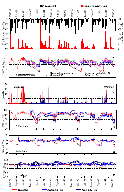
Figure C17. Soil water dynamics at Silstrup: Measured precipitation and simulated percolation 1 m b.g.s. (A), simulated and measured groundwater level (B), simulated and measured drainage flow (C), and simulated and measured soil water saturation (SW sat.) at three different soil depths (D, E and F). The measured data in B derive from piezometers located in the buffer zone. The measured data in D, E and F derive from TDR probes installed at S1 and S2 (see Figure C16).
1.1.10 Bromide Leaching
Bromide has been applied on 22 May 2000 at Silstrup. Two large storm events occurred a few days prior to and after the application of the bromide tracer. The first event caused the onset of a minor flow of drainage water, while the second resulted in rapid percolation and breakthrough of bromide to the drainage system, with the concentration reaching 5.1 mg/l on 29 May (Figure C18-B). When the bromide was applied, the groundwater table was located around 1 m b.g.s. (Figure C17-B). The presence of macropores and the location of the groundwater at the time of bromide application were reflected in the almost instantaneous occurrence of bromide in the drainage water, and suction cups S1 and S2 (Figure C18 and C19). Model simulations of the breakthrough at 1 m b.g.s. are shown in Figure C18-A and at 2 m b.g.s. in Figure C19-A. The dynamics of the breakthrough curves are well described by the model but the breakthrough occurs at the same time as the onset of continuous drainage flow (November 2000). This is about six months later than measured. Reducing the discrepancies between measured and simulated breakthrough curves in the suction cups was tried by the use of the inverse programme SUFI (Abbaspour et al., 1997) but this was not successful.
Bromide leaching to drains is well described (C18-B). Accumulated bromide leaching in the drains is shown in Figure C18-C. The simulated leaching very well corresponds to measured leaching.
Bromide has been measured below the groundwater table in monitoring wells. Because MACRO is a 1-dimensional model it is not correct to calibrate the model to concentrations below the groundwater table. Instead simulated bromide leaching below the groundwater table is evaluated against occurrence of measured bromide at same depths. Measured bromide concentration in the groundwater at 3.5 – 4.5 m b.g.s. in seven wells and simulated bromide concentration at 4 m b.g.s. are shown in Figure C19-B. The simulated leaching is in agreement with the measured occurrence of bromide.
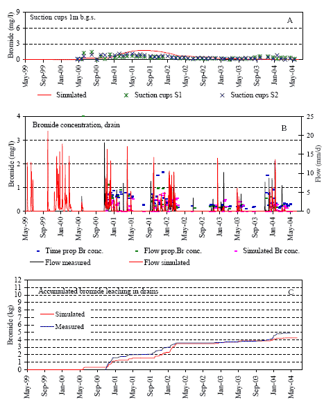
Figure C18. Simulated and measured bromide concentrations above and in the drains at Silstrup. Simulated and measured bromide concentrations at 1 m b.g.s. (A) and in drainage runoff (B). Accumulated simulated and measured bromide leaching in drains (C). The measured data in A derive from suction cups installed 1 m b.g.s. at locations S1 and S2 indicated in Figure C16.
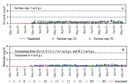
Figure C19. Simulated and measured bromide concentrations below the drains at Silstrup. Simulated and measured bromide concentrations at 2 m b.g.s. (A), measured bromide concentration in the groundwater at 3.5 – 4.5 m b.g.s, and simulated bromide concentration at 4 m b.g.s (B). The measured data in A derive from suction cups installed 2 m b.g.s. at locations S1 and S2 (Figure C16). The measured data in B derive from monitoring wells M5–M13 indicated in Figure C16.
1.1.11 Calibration of Estrup Model
The model for the Estrup site has been calibrated for the whole monitoring period to the observed groundwater table measured in the piezometers located in the buffer zone, to measured drainage flow, to time series of soil water content measured at one depth (25 cm b.g.s.) from a single soil profile S1 (Figure C20), to the bromide concentration measured in the suction cups located 1 and 2 m b.g.s, and to measured bromide leaching in drains. The model is evaluated with respect to monitoring measurements of bromide below 3 m b.g.s. The TDR probes installed at 60 cm and 110 cm b.g.s. yielded unreliable data with saturations far exceeding 100% and dynamics with increasing soil water content during the drier summer periods. No explanation can presently be given for the unreliable data, and they have been excluded from the analysis. The data from the soil profile S2 have also been excluded due to a problem of water ponding above the TDR probes installed at S2, as mentioned in Kjær et al. (2003). Because of the erratic TDR data, calibration data are more limited at this site. Data acquisition and model set-up are described in Kjær et al. (2005) appendix 4. The main calibration parameters were the empirical parameter BGRAD, which regulates the boundary flow, the “boundary” pressure head (CTEN), its corresponding water content (XMPOR), the hydraulic conductivity (KSM) and the effective diffusion path length (ASCALE), which controls the exchange of water and solute between the two flow domains (see Kjær et al. (2005) appendix 4 for details). In addition the solute concentration factor (FSTAR) is calibrated. It accounts for crop uptake of solute in the transpiration stream.
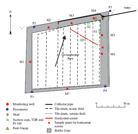
Figure C20. Overview of the Estrup site. The innermost white area indicates the cultivated land, while the grey area indicates the surrounding buffer zone. The positions of the various installations are indicated, as is the direction of groundwater flow (by an arrow). (Kjær et al., 2005)
1.1.12 Soil Water Dynamics and Water Balances
The model simulations are generally consistent with the observed data (which are more limited compared to other PLAP sites, as noted above), indicating a good model description of the overall soil water dynamics in the unsaturated zone (Figure C21). The dynamics of the simulated groundwater table is well described (Figure C21-B) and the model can capture the degree of soil water saturation 0.25 m b.g.s. (Figure C21-D). The simulated drainage (Figure C21-C) matches the measured drainage flow well.
Percolation at Estrup is shown for 0.6 m b.g.s. rather than for 1 m b.g.s. because the soil at 1 m b.g.s. is saturated for longer periods (Figure C21).
The resultant annual water balance for Estrup is shown for the five monitoring periods (July–June) in Table C14. For additional information about the water balance in the monitoring period see Kjær et al. (2005).
Table C14. Annual water balance for Estrup (mm yr-1). Precipitation is corrected to the soil surface according to the method of Allerup and Madsen (1979). 1)Monitoring started in April 2000, 2)Normal values based on time series for 1961–1990 corrected to the soil surface, 3)Groundwater recharge is calculated as precipitation - actual evapotranspiration - measured drainage, and 4) Where drainage flow measurements are lacking, simulated drainage flow was used to calculate groundwater recharge.
| Period | Normal Precipi- tation 2) |
Precipi-tation | Actual evapotrans-piration | Measured drainage | Simulated drainage | Groundwater recharge 3) |
| 1.7.99–30.6.00 1) | 968 | 1173 | 466 | – | 533 | 154 4) |
| 1.7.00–30.6.01 | 968 | 887 | 420 | 356 | 340 | 111 |
| 1.7.01–30.6.02 | 968 | 1290 | 516 | 505 | 555 | 270 |
| 1.7.02–30.6.03 | 968 | 939 | 466 | 329 | 346 | 144 |
| 1.7.03–30.6.04 | 968 | 928 | 496 | 298 | 312 | 134 |
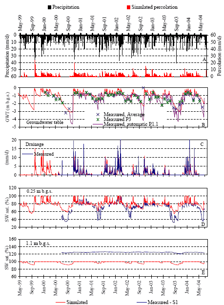
Figure C21. Soil water dynamics at Estrup: Measured precipitation and simulated percolation 0.6 m b.g.s. (A), simulated and measured groundwater level (B), simulated and measured drainage flow (C), and simulated and measured soil saturation (SW sat.) at two different soil depths (D and E). The measured data in B derive from piezometers located in the buffer zone. The measured data in D and E derive from TDR probes installed at S1 (see Figure C20).
1.1.13 Bromide Leaching
Bromide tracer was applied to Estrup in May 2000. Model simulations of the breakthrough at 1 m b.g.s. are shown in Figure C22-A and at 2 m b.g.s. in Figure C23-A. They show that the dynamics of the breakthrough are well described by the model. Simulated concentrations in drainage runoff captures well the measured concentrations (Figure C22-B) and the accumulated simulated bromide leaching in drains is consistent with measured leaching (Figure C22-C).
Bromide has been measured below the groundwater table in monitoring wells. Because MACRO is a 1-dimensional model it is not correct to calibrate the model to concentrations below the groundwater table. Instead simulated bromide leaching below the groundwater table is evaluated against occurrence of measured bromide at same depths. Measured bromide concentration in the groundwater at 3.5 – 4.5 m b.g.s. in seven wells and simulated bromide concentration at 4 m b.g.s. are shown in Figure C23. The simulated leaching is in agreement with the measured occurrence of bromide.
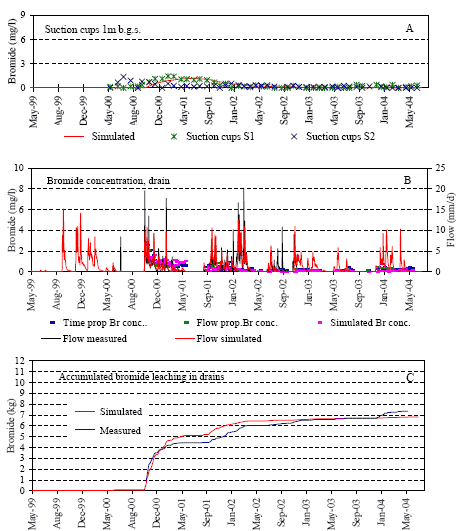
Figure C22. Simulated and measured bromide concentrations above and in the drains at Estrup. Simulated and measured bromide concentrations at 1 m b.g.s. (A) and in drainage runoff (B). Accumulated simulated and measured bromide leaching in drains (C). The measured data in A derive from suction cups installed 1 m b.g.s. at locations S1 and S2 indicated in Figure C20.
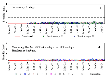
Figure C23. Simulated and measured bromide concentrations below the drains at Estrup. Simulated and measured bromide concentrations at 2 m b.g.s. (A), measured bromide concentration in the groundwater at 3.5 – 4.5 m b.g.s, and simulated bromide concentration at 4 m b.g.s (B). The measured data in A derive from suction cups installed 2 m b.g.s. at locations S1 and S2 (Figure C20). The measured data in B derive from monitoring wells M1–M7 indicated in Figure C20.
1.1.14 Calibration of Faardrup Model
The model for the Faardrup site has been calibrated for the whole monitoring period to the observed groundwater table measured in the piezometers located in the buffer zone, to time series of soil water content measured at three depths (25, 60 and 110 cm b.g.s.) from the two profiles S1 and S2 (Figure C24), to the measured drainage flow, to the bromide concentration measured in the suction cups located 1 and 2 m b.g.s, and to measured bromide leaching in drains. The model is evaluated with respect to monitoring measurements of bromide below 3 m b.g.s. Data acquisition and model set-up are described in Kjær et al. (2005) appendix 4. The main calibration parameters were the empirical parameter BGRAD, which regulates the boundary flow, the “boundary” pressure head (CTEN), its corresponding water content (XMPOR), the hydraulic conductivity (KSM) and the effective diffusion path length (ASCALE), which controls the exchange of water and solute between the two flow domains (see Kjær et al. (2005) appendix 4 for details). In addition the solute concentration factor (FSTAR) is calibrated. It accounts for crop uptake of solute in the transpiration stream.
As stated in Kjær et al. (2003), precipitation measured at Flakkebjerg 3 km east of Faardrup was used for the monitoring periods July 1999–June 2002 due to an electronic noise problem in the automated monitoring system at Faardrup.
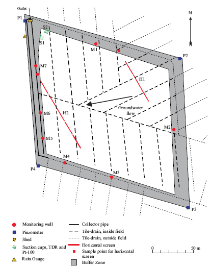
Figure C24. Overview of the Faardrup site. The innermost white area indicates the cultivated land, while the grey area indicates the surrounding buffer zone. The positions of the various installations are indicated, as is the direction of groundwater flow (by an arrow). (Kjær et al., 2005)
1.1.15 Soil Water Dynamics and Water Balances
The model simulations are generally consistent with the observed data, thus indicating a good model description of the overall soil water dynamics in the unsaturated zone (Figure C25). The dynamics and level of the measured groundwater table are well described by the present model. However, the drop in measured groundwater table during the dry summer periods is not fully reflected in the simulations. Furthermore, the measured quick rise in groundwater table after the summer period is too slow in the simulation. The level and dynamics of the soil water content in all three horizons are well described by the model (Figure C25-D, E and F).
The simulated drainage flow closely matches the measured drainage flow (Figure C25-C). However, the simulated peak at the onset of the drainage flow in the monitoring period is less well described. This is probably attributable to the above-mentioned problems with the groundwater table.
The resultant annual water balance for Faardrup is shown for the five monitoring periods (July–June) in Table C15. For additional information about the water balance in the monitoring period see Kjær et al. (2005).
Table C15. Annual water balance for Faardrup (mm yr-1). Precipitation is corrected to the soil surface according to the method of Allerup and Madsen (1979). 1) Normal values based on time series for 1961–1990, 2) For 1.7.99–30.6.02, measured at the DIAS Flakkebjerg meteorological station located 3 km from the test site (see text), and 3) Groundwater recharge is calculated as precipitation - actual evapotranspiration - measured drainage.
| Period | Normal Precipi- tation 1) |
Precipi- tation 2) |
Actual Evapotrans- piration |
Measured drainage | Simulated drainage | Groundwater recharge 3) |
| 1.7.99–30.6.00 | 626 | 715 | 572 | 192 | 147 | -50 |
| 1.7.00–30.6.01 | 626 | 639 | 383 | 50 | 31 | 206 |
| 1.7.01–30.6.02 | 626 | 810 | 531 | 197 | 169 | 85 |
| 1.7.02–30.6.03 | 626 | 633 | 483 | 49 | 75 | 102 |
| 1.7.03–30.6.04 | 626 | 587 | 435 | 36 | 0 | 116 |
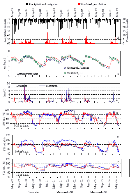
Figure C25. Soil water dynamics at Faardrup: Measured precipitation and simulated percolation 1 m b.g.s. (A), simulated and measured groundwater level (B), simulated and measured drainage flow (C) and simulated and measured soil water saturation (SW sat.) at three different soil depths (D, E, and F). The measured data in B derive from piezometers located in the buffer zone. The measured data in D, E and F derive from TDR probes installed at S1 and S2 (see Figure C24).
1.1.16 Bromide Leaching
Bromide tracer was applied to Faardrup in September 1999. Measured breakthrough curves of bromide to the drainage system 1 m b.g.s. in suction cup S1, and 2 m b.g.s. in suction cup S2 are shown in Figures C26-A and C27-A. Noting that the precipitation is not locally measured for all years, as stated previously, model simulations are able to replicate the breakthrough (Figures C26-A and C27-A). Simulated concentrations in drainage runoff captures well the measured concentrations (Figure C26-B) and the accumulated simulated bromide leaching in drains is almost consistent with measured leaching (Figure C26-C).
Bromide has been measured below the groundwater table in monitoring wells. Because MACRO is a 1-dimensional model it is not correct to calibrate the model to concentrations below the groundwater table. Instead simulated bromide leaching below the groundwater table is evaluated against occurrence of measured bromide at same depths. Measured bromide concentration in the groundwater at 3.5 – 4.5 m b.g.s. in seven wells and simulated bromide concentration at 4 m b.g.s. are shown in Figure C27-B. The simulated leaching is in agreement with the measured occurrence of bromide.
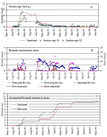
Figure C26. Simulated and measured bromide concentrations above and in the drains at Faardrup. Simulated and measured bromide concentrations at 1 m b.g.s. (A) and in drainage runoff (B). Accumulated simulated and measured bromide leaching in drains (C). The measured data in A derive from suction cups installed 1 m b.g.s. at locations S1 and S2 indicated in Figure C24.
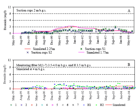
Figure C27. Simulated and measured bromide concentrations below the drains at Faardrup. Simulated and measured bromide concentrations at 2 m b.g.s. (A), measured bromide concentration in the groundwater at 3.5 – 4.5 m b.g.s and simulated bromide concentration at 4 m b.g.s (B). The measured data in A derive from suction cups installed 2 m b.g.s. at locations S1 and S2 (Figure C24). The measured data in B derive from monitoring wells M1–M7 indicated in Figure C24.
Version 1.0 August 2007, © Danish Environmental Protection Agency