| Forside | | Indhold | | Forrige | | Næste |

Frakturer fra lodrette testboringer på Vestergade 10 Haslev

Bilag D

Fracturing Activities

Vestergade 10
Haslev, Denmark
31 January 2001 – 6 February 2001

Provided to:
Vestsjællands Amt
Natur & Miljø
Amtsgården
4180 Sorø

Submitted by:

NCC Danmark A/S
Kirkebjerg Allé 85
2605 Brøndby

Brøker I/S
Spånnebæk 7
4300 Holbæk

FRx, Inc.
P.O. Box 498292
Cincinnati, Ohio
45249
USA

February 2001

Summary

Crews of NCC, Brøker Drilling I/S and FRx, Inc. created two hydraulic fractures in soils below the backyard at Vestergade 10, Haslev, Denmark. The fractures were created at two depths, approximately 4.5 m and 8m bgs, from individual wells constructed less than a half-meter apart. Each fracture contained 120 l of course or medium grained sand. Pressure data and uplift measurements indicate both fractures assumed a horizontal or sub-horizontal form.

Introduction

Purpose and Scope

This report is produced by Bill Slack form FRx and it documents fracturing work and related activities conducted in late January / early February 2001. The objective of the project was to create hydraulic fractures that can be used in a test of fracture-enhanced vapor or dual-phase extraction. Since the project also introduced the use of hydraulic fractures as remedial tools for contaminated soils and groundwater in Denmark, the project included quality control and documentation efforts to verify the form and extent of the fractures. This report includes data from those efforts.

Site Characteristics

Subsurface soils at Vestergade 10, Haslev, have become contaminated with chlorinated solvents as the result of ongoing dry cleaning operations. A memorandum by NIRAS [1999] summarizes the site characteristics and extent of contamination. The following synopsis paraphrases that memorandum.

The site soils consist of a 1 – 2 m thick layer of fill, 2 – 3 m slightly sandy, slightly silty calcareous glacial clay. From 4 – 5 m bgs the clay becomes denser. Groundwater is found in the fill and in the upper part of the till with a water table typically measured at 1 – 1.5 m bgs.

The clay soil contains natural fractures that serve as preferential pathways for groundwater and vapor movement. Measurements of fractures exposed by excavation at the nearby Haslev Gasworks documented vertical fractures with spacing of 0.3 to 1.5 m to depths of 8 m. The fluid movement through the fractures appears to be the principal mechanism of contaminant transport.

An extensive collection of soil gas, groundwater, and soil samples has identified hot spots of contamination immediately adjacent to and underneath the principal building on the site. Contamination was encountered at depths of 1.5 to 8 m bgs. The two test fracturing locations did not coincide with the hot spots of contamination.

Project schedule

Field activities were implemented over the course of the first week of February 2001. Although the scope of project involved only two fractures, the degree of monitoring, the introductory nature of the technology, and need to provide opportunities for quality control, oversight, and demonstration lead to a prolonged schedule. The dates of general field activities are listed in Table 1.

Methods

FRx routinely follows methods developed by the USEPA (USEPA [1993]) in its commercial environmental application of hydraulic fractures in North America. The techniques adopted for the work at Haslev comprise a minor variant of these traditional procedures. Specifically the Haslev injection wells were larger and were installed without a drive point. An appropriate section of open borehole was exposed by a separate augering step. Otherwise, the Haslev work closely followed the USEPA procedures. These steps include: (1) cutting a thin kerf in the wall of the borehole by means of a horizontal hydraulic jet, (2) pressurizing the kerf with liquid so as to nucleate a horizontal fracture from the hoop that constitutes its outer edge, (3) delivering sand-laden slurry to the open hole section of the well so as to propagate the fracture, and (4) monitoring the injection pressure and surface deformation, which permits deduction of the fracture form.

Drilling, Well Installation, and Notching

Two injection wells and a set of offset monitoring piezometers were installed at locations shown in Figure 1, the site map and in greater detail in Figure 2.

The injection wells were composed of 10 cm steel casing that was inserted through a 15 cm hollow stem auger. The open-ended casing was then pressed an additional 20 cm into undisturbed soil. The annular space between the augered borehole and the 10 cm steel casing was filled to surface with cement grout by tremie pipe while withdrawing augers. The surface was completed with a concrete flush mount sill and cover block. After the grout set, a 7.5 cm solid auger was used to create an open borehole 30 cm below the bottom of the steel casing. Table 2 lists the depths and available fracturing intervals for the two injection points. Figure 3 schematically illustrates the well construction.

The wells were constructed several weeks prior to fracturing activities. In the interim, 60 cm long sections of 5 cm screen were installed in the wells with appropriate riser to reach the ground surface. Recovery tests were performed upon the wells to establish baseline performance. The screens were removed upon mobilization of fracturing equipment to the site.

Piezometers with short screens were installed a multiple levels approximately 0.5, 1, 2, 3, and 5 m east^[1] and 1, 2, and 4 m north of the pair of injection locations. Locations are shown in Figure 1 and Figure 2. The 20 mm piezometers were installed in holes bored to depths of 2.20 m, 4.50 m, or 8 m with a 7.5 cm auger. The screen section of each piezometer was 30 cm in length. Piezometers were grouted in place. A packer gland fitted on the riser immediately above the screen was inflated prior to grouting to preclude occlusion of the screen.

The fracture initiation kerf was created by directing a hydraulic jet at the wall of the open borehole below the bottom of the 10 cm steel casing. The jet was suspended from the top of the casing by a stiff pipe, and the casing was open to the atmosphere. Rotation of the pipe around the axis of the well caused the jet to carve disk-shaped kerf a few millimeters thick. After cutting for several minutes, the elevation of the jet was raised 5mm and a second cut was made. The result of the two cuts was a kerf with an aperture of at least 1 cm. The jet was operated at 200 bar and 1 m³/hr. Cuttings overflowed the leg of a tee mounted on the casing and were collected in a mud pan.

Materials

The fractures were created with course-grained or medium-grained sand suspended in cross-linked guar gum slurry. Enzyme breaker was added to the slurry to promote ultimate degradation of viscosity. Materials were obtained from suppliers as listed in Table 3.

Solutions were prepared with water obtained from a tap in the basement of the house at Vestergade 10. Guar solution was prepared in a 600 l mud mixer. Stock solutions of crosslinker and breaker were mixed in 20 l buckets. Concentrations of the solutions are listed in Table 4.

Three types of sand were used. The uppermost fracture contained a 50:50 mixture of red sand and brown sand. The lowermost fracture was filled with green sand. The different colors were selected to facilitate identification of the fractures during subsequent exploration.

Mixing and Injection Equipment

Injected slurry was prepared in discrete batches of ~ 75 l. The planned ingredients of batches were measured volumetrically and set aside prior to injection.

Batches were prepared in cement mixers. The mixers were driven by 2 kW electric motors and could thoroughly mix a charge of solutions and solids in less than two minutes. The use of two mixers permitted preparation of consecutive batches without interruption of delivery.

The mixers were positioned to discharge into a hopper fixed to the suction throat of a progressing cavity pump. This type of pump tolerates the high-solids characteristics of the injection slurry while maintaining a smooth, pulseless delivery.

Monitoring

Wellhead pressures were monitored throughout injection by manual observation and record as well as by electronic measurement and datalogging. Pump discharge pressure was displayed on a gage and recorded manually. All offset piezometers were fitted with pressure gages, and a dedicated operator reviewed all at least three times during injection and three times after injection.

Surface deformation over the fracture locations, or uplift, was measured by comparing survey notes made immediately before and immediately after injection. Survey points were placed in between the two injection wells, 1, 2, 3, and 5 m east, south and west, and 1, 2, and 4 m north of the central point. Measurements were conducted through a surveyor’s level directed at graduated tapes fixed to survey stakes, which were held vertical by being driven a few centimeters into the ground. The observation station was at the western rear corner of the entrance to the back yard.

The survey equipment was also used to monitor the elevation of selected points on the house, garages, and sheds. These measurements were taken 24 hours before, immediately before, and immediately after injection. Furthermore selected points on the houses, garages and sheds were measured 24 hours after injection. The locations are listed in Table 5.

Implementation & Results

Notching

The fracture initiation kerf, or notch, in well T1 was cut on the day slurry was injected into the well. Likewise, the notch in T2 was made the same day slurry was injected. When the notching equipment was inserted into T1, approximately 30 cm of soil blocked easy passage to the bottom. This material was removed by operating the jet while lowering the final 30 cm. Presence of this material appears to have had no further consequence. The hydraulic jet was first suspended 4.3 m bgs in T1. After operating the jet for 5 minutes, the jet was raised to 4.29 m bgs and operated for 2 minutes. In contrast, no obstruction was encountered in T2. In that well the jet was suspended at 7.8 and 7.79 m and operated for 5 and 2 minutes respectively. Similar discharge of soil-laden water overflowed into the diverting tee. Cuttings were gray clay and silt with very fine white sand. Occasionally a ped of gray clay or a small stone would be recovered.

Mixing and Injection

After notching, all final preparations for data acquisition were made. Specifically, an initial round of survey measurements were made to support uplift measurements. Also, the proper installation of all pressure gages on the piezometers was verified.

Prior to injecting fracturing slurry, the injection hose was loaded with water, the speed of the injection pump was confirmed to correspond to plan, and a cap installed upon the injection well. Activation of the well head pressure datalogger was the final task before injection. Injection commenced after a final round of coordination among the injection team and data collectors. Table  lists the composition and volume of each batch material injected into each of the two wells. The total quantity of material used in each well is also listed in Table 6. Mixing and injection proceeded according to plan with essentially no spillage and no disruption in delivery.

Pressure

Well head injection pressure was continuously monitored throughout injection and recorded both manually and by datalogger. Figure 4 and Figure 5 display the pressure history during and immediately after injection. The manual and electronic record are simultaneous, except for a three-minute episode during creation of T2 when the datalogger malfunctioned and recorded negative pressures. The spurious data have been discarded.

The discharge pressure of the pump was carefully monitored during the first few minutes of injection for both fractures. The first maximum pressure, or break down pressure, was noted and is also displayed on Figure 4 and Figure 5. The breakdown pressures observed at the pump were about ¾ bar greater than recorded at the wellhead while pump propagation pressures were about ¼ bar greater. The differences can be attributed to viscous losses along the length of the injection hose and, in the case of break down pressure, to electronic limitations of capturing information of brief duration by the datalogger.

During injection, the pressure within all of the transducers was monitored by observation of pressure gages mounted on the top of the piezometers. Significant pressure was noticed in only one of the twenty gages during the creation of each fracture and minor variation was noted in one or two others. During the creation of T1, 1.4 bar was observed at MB3, approximately 1 m north of the injection well in the piezometer screened from 4.2 to 4.5 m bgs. The pressure occurred early, within the first 3 minutes of injection, but was not sustained. During creation of T2, 0.6 bar was observed 3 m east at MB7 in the piezometer screened from 7.7 to 8 m bgs. The pressure appeared within the first 2 ½ minutes and remained for at least an hour. Pressure varied during injection and actually appeared to increase slightly afterwards.

The pressure transducer and datalogger remained connected to the wellheads overnight. By the next morning, pressure in either well decreased to –0.07 bar in T1, suggesting the fluid level had fallen overnight.

Uplift

Baseline survey measurements of the uplift locations were made after cutting the notch and before commencing injection. The uplift array consisted of four rays of three or four locations. The rays were oriented along the cardinal directions to form a cross. Uplift locations were placed 1, 2, 3 and 5 m east, south and west and 1, 2 and 4 meters north. Final uplift measurements were completed within ten minutes upon completion of injection. The difference between baseline and final survey elevations is taken as uplift and is displayed in Figure 6 and Figure 7.

Uplift for both fractures assumed the pattern of a broad dome roughly, but not exactly, centered on the injection well. Each dome was somewhat elliptical, with axes ratios of 1.17 and 1.11 for T1 and T2, respectively. Maximum recorded uplift was 1.05 and 0.30 cm for T1 and T2. The inferred location for true maximum uplift, which may exceed the recorded values, did not coincide with the injection wells, but was within the range of expected locations. The dome for T1 contained 0.22 m³, which corresponds to approximately 2/3 of the volume of injected slurry. The dome for T2 was smaller – only 0.07 m³ and accounts for barely ¼ of the injected volume. These volumes and ratios are consistent with expectations for horizontal or sub-horizontal fractures, as documented in Table 11.

Other observations during fracturing

Baseline elevation measurements of survey marks were made upon six stations in or near the backyard of Vestergade 10 at least 24 hours before and immediately fracture creation. The survey locations are listed in Table 5. Corresponding elevation measurements were made immediately afterward and 24 hours latter. None of these data suggested any movement of the fixed structures at the site. These data are listed in Table 9.

After approximately five minutes of injection into T1, a crack appeared along the ground surface above the fracture. The crack extended approximately 4 meters east – west and was centered upon the injection well. The aperture was approximately 1 mm and uniform along the length. Its depth could not be gauged. The crack had either closed or was obliterated by the next morning. This crack had all the characteristics of doming cracks formed above horizontal or sub-horizontal fractures.

During the creation of T2, a small volume of fluid flowed slowly from the well that accessed T1. The discharge commenced after approximately 3 minutes of injection. A cap was installed within another two minutes. The entire discharge amounted to less than five liters. This flow had all the characteristics of fracture compression induced by the uplift of an underlying fracture.

Samples of the mix were collected from each batch right before injection. The samples were stored under similar temperature as the soil temperature in order to control the efficiency of the enzyme breaker. After 24 hours the sample showed that the gel had changed into fluid with the same viscosity as water.

Exploration for fractures by soil sampling

Several days after fracturing, soil samples were collected at four locations around the fracture wells. The first samples were collected 1 m east at depths ranging from 3.2 to 9.45 m. A distinct layer of red sand was located at 4.5 m bgs. It was inclined at an angle of 60° from horizontal and had an aperture of approximately 3 mm. A trace of green sand was detected at 8.5 m bgs. A second set of samples was collected at a location 1.5 m south of the center of the injection array. Neither red nor sand was observed, although a suspect parting at 4.75 m could be identified. Recovery (the fraction of sampler filled with soil), was 30% to 35% below 5.5 m, so the lower fracture could have been omitted from the samples. Table 10 details the exploration program.

Discussion

Fracture Form

All evidence indicates both T1 and T2 assumed a horizontal or sub-horizontal orientation for at least a portion of their propagation pathway. The first indication of fracture form became evident very shortly after the fracturing process commenced. Specifically, in both instances the injection pressure increased to a maximum of approximately 3 bar within the first minute and then decreased to approximately 1.5 bar. This behavior, known as breakdown, reflects the larger stress required to cause the soil to fail and the smaller stress required to maintain horizontal propagation. Later during injection, piezometers screened in the plane of the fracture exhibited pressure variations, indicating a direct connection from the injection well to the screened interval. For T1 the effected offset piezometer, MB8, was located 1 m north. For T2, the effect was 3 m east. We do note the absence of pressure symptoms in piezometers between the injection well and MB8 suggests the fracture T2 did not assume a horizontal form near the injection well. However, additional evidence indicates that the fractures should be classified as sub-horizontal.

The uplift patterns carry all of the characteristics of horizontal or sub horizontal fractures. Much experience has shown that these types of fractures form broad domes of uplift as opposed to extremely localized and asymmetric ground displacement, which can also include subsidence, caused by vertical fractures. The domes above horizontal fractures tend to be somewhat elliptical and are rarely centered on the injection well. Also, the inferred location of maximum uplift infrequently coincides with the injection well. The quantitative parameters of these characteristics for T1 and T2 coincide with expected values that are based on measurements from hundreds of horizontal fractures. These comparisons are made in Table 11.

Even the incidental phenomena observed during fracturing suggest the formation of horizontal or sub-horizontal fractures. During the creation of T1, a crack appeared in the ground surface and extended east and west away from the injection well. This crack resulted from the soil being lifted in a broad dome by the fracture. The upper surface of a dome created by inflation from below carries the maximum strain. Clearly the stress imparted by this strain exceeded the tensile strength of the soil, and the crack opened. This type of crack, known as a doming crack, has been observed at most other sites where horizontal fractures have been created.

The expulsion of fluid from T1 during the creation of T2 results from a similar mechanism. The inflation of T2 likewise imparts a dome that compresses the overlying fracture T1. The compressive stress is relieved in part by voiding fluid through the open well.

Finally, exploration for the fractures identified red and green sand layers at appropriate depths. These findings are the most conclusive evidence of the horizontal or sub-horizontal fracture propagation pathway.

Differences between T1 & T2

These fractures are as similar as any two fractures can be at any site. Creation utilized the same fracturing techniques, including comparable well construction, similar notching processes, the same equipment, similar injection rate, and identical sand volume. The resulting fractures exhibited similar injection pressure signatures, broad uplift domes and other characteristics of horizontal or sub horizontal fractures.

Nonetheless, some distinctions can be noted. Most strikingly, the maximum uplift observed over T2 was about 1/3 that of T1, and the uplift of T2 did not appear to extend as far as T1. The difference merits an examination of factors that did vary between the two fractures.

Two obvious and unavoidable distinctions are the depth of the fracture and the corresponding different geological and geotechnical setting. Fracture T2 was created approximately 3.5 m deeper than T1. Although both fractures were created in the same geological unit (blue clay), the uppermost fracture was created closer to the contact with overlying yellow clay and, of course, closer to the ground surface. The distinction may be relevant because the physical processes of horizontal crack formation involve the character and thickness of overlying formations.

The target fracture planes for T1 and T2 were intersected by different numbers of other wells and borings. Within the vicinity of the fracture wells, four piezometers were constructed to a depth of 8 m and eight were constructed to 4.5 m. Thus the horizontal plane at the creation depth of T1 (4.3 m) intersects thirteen well casings or piezometer screens, i.e. the well for T2, piezometers at MB2, MB4, MB6 and MB7 that extend to 8 m, and piezometers at MB1, MB2, MB3, MB4, MB5, MB6, MB7 and MB8 that extend to 4.5 m. In contrast, the horizontal plane at the creation depth of T2 (7.7 m) intersects only the piezometers at MB2, MB4, MB6 and MB7 that extend to 8 m. Ordinarily we expect wells and other strong vertical features to act as reinforcing pins that inhibit opening of the fracture aperture, so the effect of penetrating wells does not seem to be significant at this site.

Four process or operational parameters varied between the two fractures. (1) A greater concentration of breaker was used in T2. The change was made in response to the observation that residual gel from T1 had not degraded in 24 hours. The temperature of these gel samples, which had remained in the injection equipment overnight, was substantially less than soil temperature, so we were not overly concerned about breaker performance. Nonetheless, a greater concentration of breaker seemed prudent. Even at the greater concentration, breaker did not affect the rheology of the gel during the time frame of injection. This difference between the two fractures was certainly inconsequential. (2) Fracture T2 was created with a smaller volume of pad, or solid-free fluid initially injected. The injection of solid-free cross-linked gel ensures that the fracture aperture opens to a width large enough to accept sand grains. Otherwise, any solids in the first volume of injected fluid will bridge across the fracture gap and can quickly occlude the fracture and the well. The change was made because T1 demonstrated that fracture aperture opens quickly at this site and because the finer sand was used. Beyond the contribution to total injected volume, the size of the pad should not have a significant impact on final fracture form. (3) Different sand was used in the two fractures. The color of sand most certainly was insignificant, but the grain size of the green sand used in T2 was finer than the red and brown sand used in T1. Finer sand can propagate farther into the fracture crack and also more readily penetrate natural void space such as fractures. Indeed, the core recovered below 8.5 m at 1 m east of the injection wells revealed a vertical fracture with aperture approximately equal to one sand grain; it contained a layer of green sand grains. (4) Two factors appear to have reduced the viscosity of the slurry injected into T2 relative T1. The concentration of guar was purposely reduced by 10% because guar gel used in T1 seemed excessively stiff and because lesser viscosity generally yields less uplift, which for T1 was greater than targets set by the project program. While cross-linked gel with the reduced concentration appeared to be more appropriate, the addition of green sand resulted in a much more runny slurry that barely could be made to “lip” in and out of a cup.

After consideration of these factors, three mechanisms appear to contribute to the diminished uplift of T2. If the injected slurry penetrated natural void space, such as fractures or inter-granular pores, then the volume of new space (created within the fracture) would be commensurately less as would uplift at the surface. The lesser viscosity and smaller grain size could support flow from the fracture into the surrounding matrix, which is known in the trade as leak-off. However, our work has not shown leak-off to be a significant factor in shallow soil fractures whereas it is important in oil field fractures. Furthermore, the same geological matrix surrounded both fractures, and leak-off from T2 should have been mirrored in T1. Thus we must conclude that a significant amount of displacement was not registered at the ground surface. This may occur if some portion of the soil overlying T2 is sufficiently elastically or plastically compressible to adsorb the dislocation caused by the opening of the fracture aperture. Alternatively, the aperture away from the center of the fracture could be sufficiently small to remain undetected by the survey method. For example, if additional aperture of 0.3 mm occurred across an area as broad as 25 m diameter (a change undetectable by the surveying method), T2 would have as much uplift volume as T1. In weighing these two alternatives, we must consider that the soil between the two fracture elevations was dense blue clay, which is not expected to be compressible. Thus we conclude that T2 did extend farther than detected. A volumetric balance suggests that its true radius lies closer to 8 m if the fracture remained sub-horizontal.

Recommendations for Use

These fractures should perform well as enhancements to vapor or dual phase extraction processes. Application of these processes should be rather straightforward.

The best recovery from a fracture can be affected through the well used to create the fracture. These wells provide a much better connection to the fracture sand than any well that is installed afterwards, even if the additional well targets the maximum aperture. The near-impossibility of creating a well without smearing a skin of clay across the fracture frustrates any attempt to use additional wells. The well used to create the fracture also has a better connection than existing wells intercepted by fractures. The quality of a connection between a fracture and an intercepted well cannot be anticipated, and probability based on experience appears to favor the fracture creation well. In the light of these arguments, the plan to test process performance through the two injection wells is sound. We note the well design ingeniously permits performance testing before and after creation of the fractures.

The following steps should be respected during the conversion of the wells from fracture creation wells to extraction wells. In aggregate, these individual procedures will result in optimal well performance.

First, all excess sand should be removed from the wells either by augering or flushing. The bottom 30 cm of open borehole should be cleaned carefully and as deeply as possible. During this cleaning care should be exercised to avoid skinning the fracture face with clay or washing sand out of the fractures. The potential for the later problem will be much attenuated when the gel is broken. If the gel does not appear to be sufficiently broken, i.e. blobs of sand in viscous or semi-viscous liquid can be recovered from the well, then an oxidizing solution should be pumped into the well. A 20 l dose of 10% sodium hypochlorite (NaClO – a common laundry bleach) should affect total break down within a day.

The well screens used during previous performance tests should be cleaned and reinserted into the wells as deep as possible. The wells will perform best if fluid can be drawn down below the fracture face. The fracture can be exposed if the pump or aspiration inlet can be positioned near the bottom of the 30 cm borehole. Thus deep screens will prove advantageous.

Recovery tests should include measurements of pressure (draw down or vacuum) as well as volumetric rate. Tests should be conducted at three or four sets of pressures and rates. The ratio of rate versus pressure, in whatever units, is a measure of the deliverability of fluid through the fracture. Collection of multiple sets of pressure and rate permit assessment of average deliverability, i.e. characterization of performance over a range of operating conditions. We have routinely observed that the deliverability of fractures exceeds the deliverability of conventional wells by factors of 20 to 50.

Conclusions

Both fractures appear to be horizontal or nearly so. The injection pressures exhibited classic signatures for sub-horizontal fractures. The upward deformation of the ground surface, or uplift, assumed the characteristic broad and elliptical dome of horizontal fractures. Pressures were observed during injection at appropriate elevations in offset piezometers, which could only result from lateral propagation of the fracture. Likewise, distinctly identifiable fracture traces and fracture sand were found at appropriate elevations in soil cores collected after fracturing.

The fracturing process in the clay tills at Haslev appears to be tolerant of offset wells that penetrate the fracture plane. In particular, fracture T1, which was created at 4.5 m bgs, cut across thirteen wells or piezometers that extended past the depth of the fracture. These were located at distances of 0.45 m to 5 m from the injection well and were concentrated on the east and north side. No effect on the symmetry of T1 could be discerned.

Although relatively small with respect to the maximum size that might be possible at Haslev, the fractures should prove to be significant enhancements to fluid recovery operations such as dual phase extraction.

Tables and Figures

Table 1 Implementation Schedule

Table 2 Well Specifications

Table 3 Material Specifications

Table 4 Solution Concentrations

Table 5 Locations of Survey Control Stations

Table 6 Injection Schedule

Table 7 Pressure In Offset Piezometers During Injection of T1, 4.5 m. Pressures reported in bar. One person observed pressure gages mounted on the piezometers during injection. Each of six cycles of observation includes one record of each piezometers. Each cycle required two to three minutes to complete. Bold font indicates piezometers where change was noted during injection.

Table 8 Pressure In Offset Piezometers During Injection of T2, 8 m. Pressures reported in bar. One person observed pressure gages mounted on the piezometers during injection. Each of six cycles of observation includes one record of each piezometers. Each cycle required two to three minutes to complete. Bold font indicates piezometers where change was noted during injection.

Table 9 Survey Data. Uplift as well as benchmark elevations.

Click here to see Table 9

Table 10 Explorations by Soil Sampling. Pushing a tubular sampler collected soil cores 1 m long x 5 cm diameter. Drilling with a 7.5 cm auger advanced intervals between samples.

† Recovery refers to the fraction of sampler that is filled with soil.

Table 11 Uplift Characteristics. The quantitative description of uplift above horizontal fractures has been developed from measurements for hundreds of fractures. Parameters from Murdoch et al. [1995].

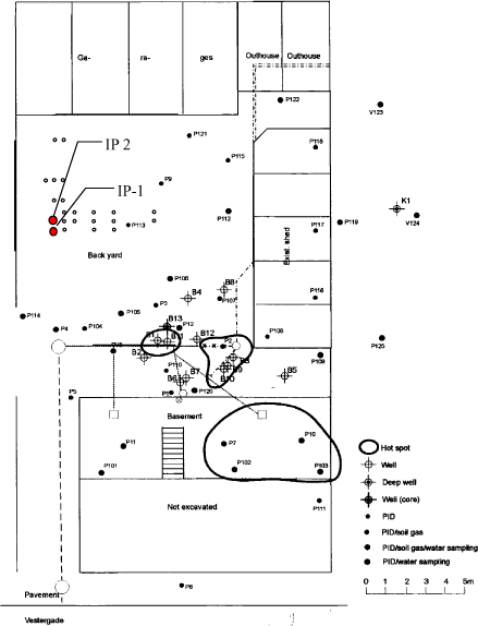
Figure 1. Site Map. Hydraulic fractures were created in the backyard relatively remote from contaminant hotspots underneath the house at Vestergade 10. Solid circles indicate injection wells. Open circles indicate piezometers. Details of piezometer placement are better shown on uplift maps, Figure 6 and Figure 7. Hot spots, other wells and borings, and sampling locations indicated by the legend.

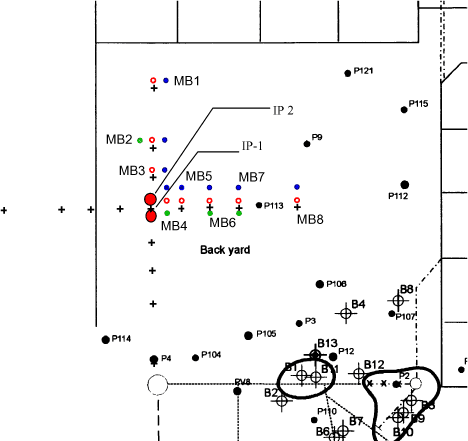
Figure 2 Detail of Fracturing Site Layout. Uplift locations shown as crosses. Injection wells indicated as large red circles. Eight monitoring piezometers screened between 1.9 and 2.2 m bgs shown as blue, filled circles. Eight piezometers screened between 4.2 and 4.5 m bgs shown as open circles. Four piezometers screened from 7.7 to 8 m bgs shown as light green circles.

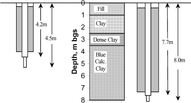
Figure 3. Schematic of Well Construction. Both T1 and T2 were constructed with 10 cm steel casing inserted open-ended through hollow stem auger and pressed an additional 20 cm into undisturbed soil. Annular space between the augered borehole and the 10 cm steel casing was filled with cement grout by tremie pipe while withdrawing augers. After the grout set, a 7 cm solid auger was used to create an open borehole 30 cm below the bottom of the steel casing. Not to scale.

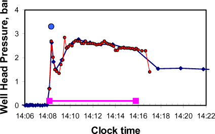
Figure 4 Pressure Log For Fracture T1. Injection pressure as measured by a transducer mounted on the well head and recorded by the datalogger shown as blue diamonds. The manual record of wellhead pressure shown as red circles. The solitary large blue circle indicates break down pressure observed at the pump discharge. The straight horizontal line that connects two squares indicates the duration of injection.

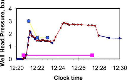
Figure 5. Pressure Log For Fracture T2. Injection pressure as measured by a transducer mounted on the well head and recorded by the datalogger shown as blue diamonds. The datalogger malfunctioned from 12:23:40 until 12:27:40. The manual record of wellhead pressure shown as red circles. Similarities of electronic and manual data before and after this episode suggest manual data provides an accurate depiction of injection pressure. The three large blue circles indicate observed pump discharge pressure, including breakdown pressure. The straight horizontal line that connects two squares indicates the duration of injection.

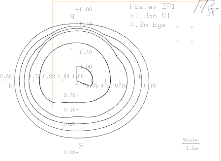
Figure 6 Uplift above Fracture T1. Uplift measured at locations indicated by + and recorded in cm. Axes indicate north / south and east / west distances in meters from center of uplift array. Injection occurred at a location 22.5 cm north of the center of the array. Contours drawn by bi-linear interpolation in an orthogonal r-q reference frame among sets of selected locations. Contours shown for 0.1, 0.15, 0.20, 0.25, 0.5 and 1.0 cm of uplift. Perimeters of garages and outbuildings and location of wooden fence indicated by light straight lines. Approximate location of slug test wells shown by small dark blue double triangles. Location of piezometers installed to 2.2, 4.5, and 8.0 m bgs shown as blue single triangles, yellow circles, and small purple squares, respectively.

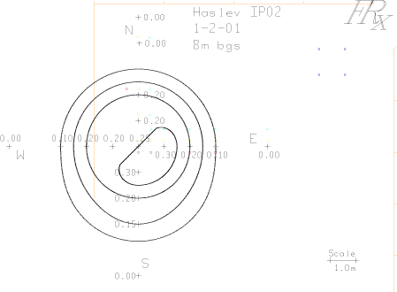
Figure 7 Uplift above Fracture T2. Uplift measured at locations indicated by + and recorded in cm. Axes indicate north / south and east / west distances in meters from center of uplift array. Injection occurred at a location 22.5 cm south of the center of the array. Contours drawn by bi-linear interpolation in an orthogonal r-q reference frame among sets of selected locations. Contours shown for 0.1, 0.15, 0.20 and 0.25 cm of uplift. Perimeters of garages and outbuildings and location of wooden fence indicated by light straight lines. Approximate location of slug test wells shown by small dark blue double triangles. Location of piezometers installed to 2.2, 4.5, and 8.0 m bgs shown as blue single triangles, yellow circles, and small purple squares, respectively.

References

Murdoch, L.C., D. Wilson, K. Savage, W. Slack, and J. Uber. “Alternative Methods for Fluid Delivery and Recovery”. USEPA/625/R-94/003. 1995.

For entire document download in PDF format: www.epa.gov/ordntrnt/ORD/WebPubs/fluid.html

For page-by-page on-line viewing: www.epa.gov/clariton/clhtml/pubtitle.html (search for 625R94003)

Rens, Rekord, “Summary of Soil and Ground Water Investigations at Vestergade 10,” Niras, June 1999.

USEPA. Risk Reduction Laboratory and The University of Cincinnati. “Hydraulic Fracturing Technology - Applications Analysis and Technology Evaluation Report” USEPA/540/R-93/505. 1993.

For entire document download in PDF format: www.epa.gov/ORD/SITE/reports/051.htm

For page-by-page on-line viewing: www.epa.gov/clariton/clhtml/pubtitle.html (search on that page for 540R93505)

Nomenclature and Abbreviations

bgs – below ground surface
USEPA – United States Environmental Protection Agency

l – liter

m – meter
cm – centimeter
mm – millimeter

hr – hour
min – minute
sec – second

kW – kilowatt

Fodnoter

^[1] The cardinal directions used throughout this report are arbitrarily oriented with the property boundaries. North in this report is taken to be parallel to property lines extending away from the street.

| Forside | | Indhold | | Forrige | | Næste | | Top |

Version 1.0 August 2006, © Miljøstyrelsen.