[Front page] [Contents] [Previous] [Next] |
Point and non-point source leaching of pesticides in a till groundwater catchment
5. Numerical modelling
Objectives and issues
The objective of the modelling was to give an estimate of pesticide leaching from the till sequence into a main reservoir. This includes modelling of laboratory tracer experiments on undisturbed columns, and considerations on upscaling of experimental laboratory data to the geological scale. The chapter also includes transport analysis of the distribution of tritium (profiles presented in Figure 9), sensitivity analyses to identify important factors in case of fracture flow, considerations about the predictability of the transport, and modelling methodology (fractured media flow versus porous media flow).
5.1 Groundwater modelling
A steady-state, three-dimensional numerical groundwater flow model of the sand and chalk aquifers underlying the Skćlskřr site was calibrated with the objective of estimating the flux of groundwater through the overlying till.
5.1.1 Computer Code
MODFLOW
The computer code used to simulate groundwater flow is the USGS's Modular Three-Dimensional Finite-Difference Ground-Water Flow model (McDonald and Harbaugh, 1988), commonly referred to as MODFLOW. This code solves the mathematical equations that describe groundwater flow in three dimensions using a finite-difference approach that estimates hydraulic head and flow as functions of time and space. This code was chosen because of its flexibility in evaluating various aquifer conditions, relative ease of use, and accuracy.
5.1.2 Conceptual Model
ZEUS database and hydrogeology
The conceptual model of hydrogeology of the Skćlskřr area was developed from borehole logs, and groundwater level data obtained from the ZEUS database (Gravesen & Fredericia, 1984), Vestsjćlland County and Skćlskřr water supply. The groundwater system is conceptualized as consisting of a shallow till underlain by sand and limestone aquifers. The till is recharged by precipitation. Groundwater flow within the till consists of a horizontal component which discharges to surface water bodies and agricultural drains, and a vertical component which discharges to the underlying sand an chalk aquifers. The sand and chalk aquifers are confined and are recharged solely from vertical flow through the till. A clay unit present in the northeastern corner of the model area separates the sand and chalk aquifers. The groundwater discharges from the aquifer system to the sea and from the extraction wells within the sand and chalk aquifers.
Objective of MODFLOW mode
The objective of the MODFLOW modelling is to estimate the vertical groundwater flux or recharge from the till to the underlying aquifers. Therefore, the system was further simplified to consist of a sand aquifer underlain by a limestone aquifer. The interaction with the overlaying till is conceptualized as a recharge boundary where land is present and a discharge boundary where the sea is present. The model area is presented in Figure 16. Maps of the potentiometric surface of the sand and chalk aquifers are presented in Figure 17 and 18. Horizontal groundwater flow directions within these aquifers generally radiate from inland topographic highs and are perpendicular to the coastline.
Transmissivity estimates for the sand and chalk aquifers were obtained from the ZEUS database and from pumping tests made by Skćlskřr water supply. Transmissivity values for the sand aquifer range from 5×10⁻⁶ to 2×10⁻² m2/day. For the limestone aquifer the range is 1×10⁻⁵ to 1×10⁻³ m2/day.
5.1.3 Model Area and Grid
The model domain is presented in Figure 16. It encompasses a rectangular area of 22.350 metres (east-west) by 16.885 metres (north-south). A non-uniform model grid was used. Grid cell dimensions are 100 metres by 100 metres in the vicinity of Skćlskřr and increase to 1000 metres by 1000 metres along the model boundaries.

Figure 16
Area of numerical groundwater modelling
Grundvandsmodelleringsomrĺde
5.1.4 Layers
The groundwater flow model consists of two layers which represent the sand and chalk aquifers. The thickness of the sand aquifer is represented in the model as zones of 0, 10, 20, and 30 m. The thickness of the chalk aquifer is held constant throughout the model area and is specified as 50 m. The clay which is locally present between the sand and chalk aquifers was represented implicitly in the model by the specification of a vertical conductance term. A constant thickness of 20 m and a vertical hydraulic conductivity of 1×10⁻⁹ m/s was assumed in the calculation of the vertical conductance of this clay layer.
5.1.5 Calibration Data
Available groundwater level data for the model area are limited. The ZEUS database was queried for groundwater level data for the sand and chalk aquifers for the time periods of 1940 to 1960, 1960 to 1980, and 1980 to 1994.
Groundwater levels
The groundwater level data represents a mixture of water levels at the time of drilling and measurements in completed wells. Additionally these data are a composite of water levels representing different times of the year and wet and dry years. However, it is assumed that the data sets represent average water levels for each time period. Comparisons of contour

Figure 17
Equipotential map of the sand aquifer
Ćkvipotentiale kort over det primćre sand grundvandsreservoir

Figure 18
Equipotential map of the limestone main aquifer
Ćkvipotentiale kort over det primćre kalkstensgrundvandsreservoir
maps of the groundwater levels for these time periods did not reveal any trends in water levels. The water level data for the time period of 1980 to 1994 (Figure 17 and 18) was chosen for the calibration data set.
5.1.6 Boundary Conditions
The boundary conditions for the model are shown on Figure 19. the upper surface of the model (top of sand aquifer) is simulated as a constant flux boundary, representing recharge to the sand and chalk aquifers from the till. The lower surface of the model (bottom of the chalk aquifer) is
Discharge of system
simulated as a no-flow boundary. Discharge from the two aquifers to the sea is dependent upon the head difference between the sand aquifer and sea level, the vertical conductance term which represents the vertical hydraulic conductivity and the thickness of the till unit. A head-dependent boundary was used to simulate the interaction between the aquifers and the sea. A conductance term for the till was calculated from an assumed constant thickness of 20 m and a vertical hydraulic conductivity of 1×10⁻⁹m/s.

Figure 19
Column diagram depicting the model boundary conditions
Randbetingelser for grundvandsmodelleringen
The northern and eastern boundaries of the model were originally specified as no-flow boundaries. These boundaries are approximately perpendicular to contours of the hydraulic head in each aquifer and therefore approximate streamlines. Furthermore, by setting no-flow condition at the northern and eastern boundaries, the recharge to be modelled is reduced to the upper surface recharge. However, the northern and eastern boundary conditions had to be modified to include the specification of some model cells as constant head, in order to simulate the head difference of approximately 5 m between the sand and chalk aquifers in the northeast corner of the
Values of constant head area
model area. Values of constant head were based upon the contour map of the observed groundwater levels. Groundwater extraction in the sand and chalk aquifer was simulated using sink terms which represent pumping wells. The locations and pumping rates of these extraction wells are shown on Figure 20.
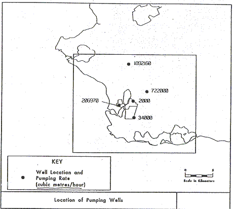
Figure 20
Location of extraction wells and rates of pumping within the model area
Lokalisering af indvindingsboringer i modelomrĺdet med angivelse af pumperater
5.1.7 Calibration
Fitting procedure
The model was calibrated by specifying the recharge rate and varying the transmissivity of the sand and chalk aquifers within reported ranges, and adjusting the recharge until an acceptable fit was obtained between observed and simulated steady-state hydraulic heads. It was by using several different combinations of recharge rates and transmissivity values determined that the model could adequately simulate the observed hydraulic heads in the sand and chalk aquifers. The model results indicate that the vertical groundwater recharge through the till sequence is 30 to 60 mm/year. These values compare favourably with recharge estimates of 37
Adjacent studies
to 46 mm/year from the till to underlying aquifers reported by Christensen (1994) for an adjacent area north of the present study area.
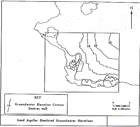
Figure 21
Simulated steady state equipotential lines of the sand aquifer
Simulerede ćkvipotentiale linier i sandreservoir
Simulated groundwater levels in the sand and limestone aquifers are presented in Figure 21 and 22. The levels are simulated by using a recharge of 40 mm/year and transmissivity values of 1×10⁻⁴ - 1×10⁻³ m2/s and 2.5×10⁻³ m2/s for the sand and chalk aquifers, respectively.
5.2 Modelling of undisturbed columns
Figure 23 a,b show the CaCl2 breakthrough curves for five undisturbed columns from the undisturbed columns at the point source site and the orchard. The curves are represented as normalized concentrations versus
Computer codes
cumulative volume of effluent (in litres). Using the codes 2D-FRACTRAN
Computer codes (Sudicky and McLaren, 1992) and CRAK (Sudicky, 1988) the breakthrough curves been modelled. 2D-FRACTRAN simulates steady-state groundwater flow and transient contaminant transport in porous or discretely fractured porous media. CRAK works under the assumption that advection only occurs in the fractures (disregards flow in the matrix) but includes matrix diffusion. In 2D-FRACTRAN, fractures can have variable length and spacing. CRAK only handles one set of equal aperture fractures with constant spacing. Since CRAK only allows advection in the fractures, the flow velocity is overestimated; however, compared with other model
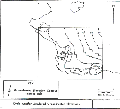
Figure 22
Simulated steady state equipotential lines of the limestone main aquifer
Simulerede ćkvipotentiale linier i det primćre reservoir
uncertainties, this assumption is considered to be of minor importance. In both models fracture walls are simplified as parallel planar surfaces.
The aim of the modelling is to achieve estimates of the aperture and spacing for the conductive fractures of the undisturbed columns. Fracture and porous media properties of the seven columns are listed in Table 10. Parameter values used for the modelling of column experiments and the following field scale modelling are show in Table 11.
Table 10
Column data used for modelling
Data anvendt i modellering af forsřg med intakte jordsřjler
Column |
Fracture spacing in cm |
Poro-sity |
Gra- |
Tracer |
Km** |
Kb |
||||
Vertical |
Horizontal |
Ton |
Toff |
|||||||
1.+2. order |
3. order |
1.+2. order |
3. order |
|||||||
| Columns from the orchard | ||||||||||
1* 2 3* |
5-7 5-10 10-20 |
10-12 5-10 18-20 |
1-2 |
30 30 25 |
0.3 4 |
0 - 0 |
168 - 172.3 |
5×10⁻¹⁰ 5×10⁻¹⁰ 5×10⁻¹⁰ |
2×10⁻⁷ 7.2×10⁻⁹ 6×10⁻⁹ |
|
| Columns from the point source site | ||||||||||
1 2* 3* 4* |
20-25 25-30 25-30 15-20 |
2-3 2-3 2-3 |
25
15-20 |
1.0-1.5 0.5-1.0 1.0-1.5 0.5-1.0 |
30 30 25 30 |
3.5 5.0 1.0 |
- 0 0 0 |
- Ą Ą 1608 |
5×10⁻¹⁰ 5×10⁻¹⁰ 5×10⁻¹⁰ 5×10⁻¹⁰ |
1.2×10⁻⁸ 2×10⁻⁸ 1.1×10⁻⁸ 7×10⁻⁸ |
*
columns with a CaCl2 breakthrough curve**
based on Foged & Wille, (1992)Table 11
Base case values of material properties used for modelling of column experiments and field
scale examples
Materiale vćrdier anvendt til modelling af sřjleforsřg og feltskala eksempler
Parameter |
Value |
Unit |
| Matrix permeability Porosity Viscosity (at 10°C) Gravitational acceleration Effective diffusion coefficient: Chloride Tritium Retardation factor: Chloride Tritium Input concentrations |
5×10⁻¹⁰ 0.25 1.31×10⁻³ 9.81
6.0×10⁻¹⁰ 7×8×10-10 1 1 1 |
m/s kg/ms m2/s
m2/s m2/s |
Conductive fractures were identified in the columns after infiltration of a fluorescent dye tracer. The total porosities are from a similar till at Enř (Fredericia, 1991). The gradients are average values for the tracer experiments and the bulk hydraulic conductivities (Kb) are calculated from
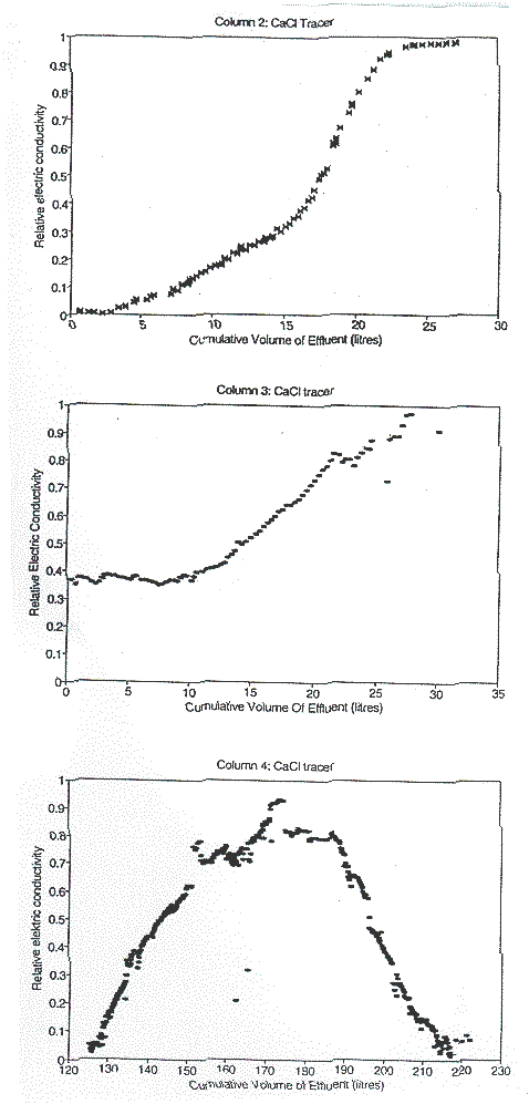
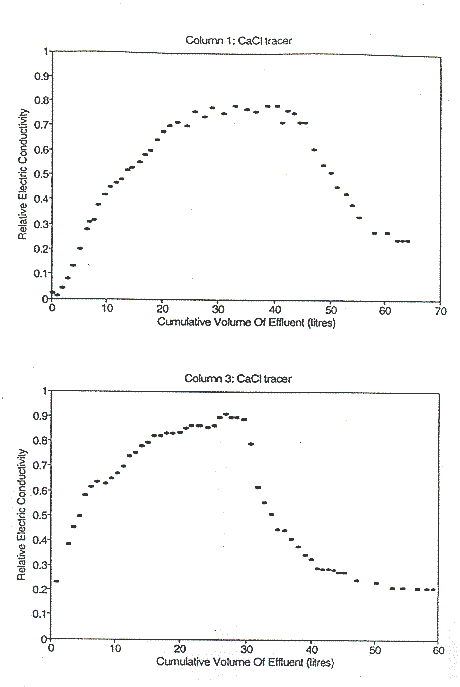
Figure 23
Transport of applied CaC12 tracer in Columns 2, 3 and 4 from the machinery yard
(point source) and Columns 1 and 3 from Skćlskřr orchard
Transport af tilsat CaC12 tracer til undersřgelse af stoftransport i sřjlerne 2, 3 og 4 fra maskinplads (punktkilde) og 1 og 3 (Skćlskřr frugtplantage)
the gradients and volumetric flow rates. Ton and Toff represent the beginning and end of the chloride tracer application. During the infiltration experiment, the hydraulic conductivity of columns was not constant (due to generation of gas in the columns). This has resulted in some unreproducible changes in CaCl2 breakthrough for column 3 (point course site) at about 550 hours.
Fracture apertures and spacing
Modelling the breakthrough curves for the undisturbed columns from the orchard, results in larger active fracture spacings than observed from the distribution of dyed fractures after the experiment, Table 12. The reason for this discrepancy may be that the major part of the flow is in some, but not all of the fractures. Oppositely, modelling of the columns from the point site results in fracture spacings smaller than measured from dyed fractures in the columns. This may reflect local differences in the till; at the point site the till contained only a few not very pronounced larger fractures. This is also indicated by the breakthrough curves which are characterized by flow in the total porosity.
Table 12
Modelled and measured active fracture spacing
Modellerede og observerede sprćkkeafstande
Modelled active fracture spacing |
Modelled fracture aperture |
Measured active fracture spacing |
|
| Column 1, orchard | 0.35 m |
48 mm |
0.05 m-0.07 m |
| Column 3, orchard | 1.0 m |
21 mm |
0.1 m-0.2 m |
| Column 2, point source | 0.12 m |
11 mm |
0.30 m-0.25 m |
| Column 3, point source | - |
- |
0.25 m-0.30 m |
| Column 4, point source | 0.05 m |
21 mm |
0.15 m-0.20 m |
As the flow rate of column 2 from the point source site changed after 550 hours, only data prior to 550 hours were used for modelling this column. For column 3 from the point source site, it was not possible to match the late but steep increases in the CaCl2 breakthrough curve.
5.3 Field scale numerical modelling of transport
Objectives and strategy
The undisturbed columns and the field measurements of fractures represent the upper 0-6 m of the till. Fracture occurrent, density and distribution below this depth is uncertain because no direct measurements exists. To evaluate the influence of deep fractures on transport, the tritium profiles (shown in Figure 9) are modelled in the following section using a fracture modelling approach versus an EPM-modelling approach.
5.3.1 Upscaling of fracture flow from columns
Procedure of upscaling
The fracture density and the hydraulic parameters of the low part of the till may be assumed to resemble the distribution observed in the large undisturbed columns. The following procedure was used for vertical extrapolation of the fracture data: Fracture apertures in the large undisturbed columns have been estimated from the CaCl2 experiments. Given the fracture and the hydraulic gradient measured in the field, the fracture density can be calculated either by using the difference in bulk and matrix hydraulic conductivity or by using the estimated amount of groundwater recharge in the area.
Hydrogeology of base case fracture model
In the upscaling, transport through a layer of 20 m till has been simulated by varying the fracture spacing and aperture, for a fixed bulk hydraulic conductivity (calculated from the recharge (q = 40 mm/year) and the gradient (i=0.2) using the formula q=K x where q=recharge). A matrix hydraulic conductivity of 5x10⁻¹⁰ m/s was assumed (reported by Foged and Wille (1992) for a similar till). In this case fractures contribute with more than 90% of the bulk hydraulic conductivity (6x10⁻⁹ m/s as estimated by the water balance modelling, section 5.1.6). The fracture aperture of 21 mm estimated in column 3, orchard (Table 11) is selected to represent the fracture throughout the till sequence. Fracture spacing was fitted (0.45 m) to produce the bulk hydraulic conductivity 6.0x10⁻⁹ m/s. The vertical flow in the set-up is 38 mm/year at a hydraulic gradient of 0.2 m (field measured
Influence of drains and interflow
mean value). The flow resembles the calibrated recharge of 40 mm/year (+20/-10). This value is significantly less than the net precipitation-evaporation) 150 mm/year, and consequently a large part of the discharge in this area must be by tile drains and by horizontal flow in the uppermost part of the till where fractures are most frequent. Possibly also small sand layers may, if interconnected, contribute to the horizontal flow.
5.3.2 Modelling of tritium profiles
Hydrogeological models
The overall hydrogeological setting used for both the fracture modelling and EPM modelling approaches is the 20 m deep aquitart with a vertical recharge of 38 mm/year. This setting is also used (unless otherwise is specified) for the sensitivity analysis of fracture transport presented in the following section.
Fracture approach versus EPM approach
In the fracture modelling approach the till is represented by the fractured aquitard derived in the previous section. In the EPM modelling approach the till is represented by a homogenous aquitard having the same bulk hydraulic conductivity as in the fracture case. Hydraulically the EPM set-up is motivated by the test carried out with the unfractured till matrix from the point source site (Table 3). The tests showed matrix hydraulic conductivities of 1x10⁻⁹ and 2x10⁻⁹ m/s. These values are in the same range (within range of uncertainty) as the estimated field scale bulk hydraulic conductivity (6x10⁻⁹ m/s) and as the deep large undisturbed columns (Table 3). The results suggest that at the field scale, fracture contribution to vertical bulk flow, may be very small or absent with depth in the till.
Tritium input in modelling
By modelling, the vertical transport of the peak tritium "pulse" infiltrated in 1963 is simulated. Sensitivity of applying this simplified tritium input versus a complete tritium input function is tested and discussed by Jřrgensen and Spliid (1997). Values of fracture and porous media properties used in the modelling are given in Table 11.
Results of modelling
The observed and modelled tritium profiles are shown in Figure 24. It appears that the EMP (no fractures) simulated tritium distribution resembles both the depth of the tritium peak values and the maximum depth of tritium occurrence in the till. In contrast the fracture simulation predict deeper penetration of the tritium peak and tritium occurrence throughout the till, which is not consistent with observations.

Figure 24
Measured and simulated depth in the till sequence of tritium peak values and lower
termination. Measured profiles are from point source site (monitoring wells 2 and 3) and
orchard (monitoring well 4). Tritium transport was simulated from a single year tritium
in-put (corresponding to peak tritium concentration in precipitation in 1963). Vertical
recharge in the simulations is 30 mm/y which is estimated from the water balance modelling
Mĺlte og simulerede dybder i till-sekvensen af tritium maximum af undergrćnsen for tritium. Mĺlte profiler er fra punktkilden (motineringsboring 2 og 3) og frugtplantagen (moniteringsboring 4). Tritium fordelingen er simuleret ud fra et enkelt ĺrs tritium-input i infiltrationen svarende til 1963 maxima. Vertikale strřmningshastighed er 30 mm/ĺr svarende til den vertikale grundvandsdannelse estimeret ud fra vandbalance modellering
Conclusion
In conclusion, the modelling indicate that the influence of fractures on chemically conservative transport at the field scale is small or absent at depths below the upper few metres at the field sites. Hence, realistic modelling results of chemically non-reactive contaminant transport may be obtained with an EPM model using the bulk hydraulic conductivity of
6x10⁻⁹ m/s (estimated by the water balance modelling).
5.4 Sensitivity analyses
The sensitivity analysis is conducted with the same base case geological framework (unless otherwise is specified) as used in the previous section, i.e. 20 m fractured clayey till overriding an aquifer, and a vertical recharge of 38 mm/year.
Flow and contaminant transport is highly sensitive to fracture aperture (flow is a cubic function of fracture aperture). A series of simulations with increasing fracture apertures have been conducted. In all simulations, the vertical recharge is constant (achieved by increasing fracture spacing to out-balance increasing aperture), Figure 25.

Figure 25
Simulated breakthrough of non-reactive tracer (chloride) through 20 m of fractured till. Breakthrough curves to the main aquifer are shown for different fracture spacings and fracture apertures at constant hydraulic conductivity of the till. For 1% of infiltrated concentrations to arrive in the main aquifer within 10 years, fracture apertures of 31 mm or more are required (the legend in the topright corner shows couples of fracture spacing and aperture values used in the simulations)
Simuleret gennembrud af en non-reaktiv tracer (klorid) gennem 20 meter sprćkket morćneler. Gennembrudsgiver til det primćre grundvandsmagasin er vist for forskellige kombinationer af sprćkkeafstande og sprćkkeaperturer ved konstant bulk hydraulisk ledningsevne. For sprćkkeĺbninger střrre end 31 mm nĺr gennembruddet en relativ koncentration pĺ 1% af udgangskoncentrationen inden for 10 ĺr
In table 13 is shown (summarizing Figure 25) the number of years for a chemically conservative tracer to arrive in the underlying aquifer at three concentration levels. The level of 1 ‰ of the input concentration is reached after 10 years at a fracture aperture of approximately 30 mm.
Table 13
Years for a chemically conservative tracer to break through 20 m of fractured till (i = 0.2) at three concentration levels
Antal ĺr for konservativt stof gennembrud pĺ tre koncentrationsniveauer gennem 20 meter sprćkket morćneler (i = 0,2)
| Fracture spacing and aperture | Contraction relative to input concentration |
||
1 ‰ |
1 % |
10 % |
|
| 1 m/21 mm | 36 |
> 40 |
> 40 |
| 2 m/24 mm | 14 |
22 |
> 40 |
| 3 m/31 mm | 6 |
10 |
24 |
| 5 m/37 mm | 2.5 |
3.5 |
9 |
| 10 m/47 mm | - |
< 1 |
2.5 |
The results shows that if widely spaced (> 10 m), highly conductive fractures occurred in the aquitard (not exposed in the field excavations or represented by the columns), the transport can be significantly faster than predicted from the upscaling based on field measurements and data from the undisturbed columns. Evaluated from the angled tritium profiles, however, there is no indication that such a flow system occurred, i.e. there is no lateral variations in tritium concentrations (Figure 9) which should be the result of matrix diffusion from conductive fractures. The observed tritium profiles have lateral homogenous tritium fronts, and at depth, the values below the limit of detection limit are stable over vertical and horizontal distances of more than 10 m in the profiles.
Numerical analysis of the lateral tritium distribution as function of widely spaced highly conductive fractures is presented in Jřrgensen and Spliid (1997).
The amount of recharge was used to calculate the bulk hydraulic conductivity of the till in section 5.1.7. The following simulations show the effect of recharge in the range of 30 mm/year to 60 mm/year (range of uncertainty), if the change in hydraulic conductivity is adjusted by changing the fracture aperture, Table 14 and 15.
Table 14
Input parameters for sensitivity analysis of recharge
Parametre anvendt til fřlsomhedsudstyr af grundvandsdannelse for konservativt stof gennembrud gennem 20 m sprćkket morćneler
Recharge |
Gradient |
Kb |
|
| Run 1 | 0.03 |
0.2 |
4.8 · 10-9 |
| Run 2 | 0.06 |
0.2 |
9.5 · 10-9 |

Figure 26
Breakthorugh to main aguifer to a non-reactive solute (chloride) at recharges of, a) 30
mm/year and b) 60 mm/year. Flow system as in previous figure
Gennembrud til det primćre reservoir af non-reaktivt stof ved grundvandsdannelser pĺ a) 30 mm/ĺr og b) 60 mm/ĺr. Samme strřmningssystem som i foregĺende figur
Table 15
Years for a chemically conservative tracer (chloride) to break through 20 m of fractured
till (i = 0.2 and spacing 3 m)
Antal ĺr for konservativt stof gennembrud pĺ tre koncentrationsniveauer gennem 20 meter sprćkket morćneler med sprćkkeafstand pĺ 3 m ved tre sprćkkeaperturer (i = 0,2)
| Recharge, aperture | Concentration relative to input concentration |
||
1 ‰ |
1 % |
10 % |
|
5 |
0.3 |
2 |
5 |
10 |
4.5 |
7.5 |
18 |
15 |
11 |
17 |
> 40 |
20 |
18 |
30 |
> 40 |
Figure 26 shows the simulated breakthrough of a non-reactive contaminant to the main aquifer for recharges at 30 mm/year and 60 mm/year. From the simulations it appears that the contaminant arrival time charges significantly within the uncertainty of recharge.
Aquitard thickness
The influence of aquitard thickness on the breakthrough of a non-reactive contaminant to the main aquifer is shown for aquitart thickness of 5 to 20 m in Figure 27. Corresponding arrival times are summarized in Table 16.
Table 16
Years for a reactive tracer (retardationfactor = 3) to break through 20 m of fractured
till as a function of till thickness (i = 0.2 fracture, spacing 3 m and fracture aperture
= 31 mm)
Effekt af morćnetykkelse pĺ antallet af ĺr for en adsorberende tracer (retardationsfaktor = 3) stof gennembrud til tre koncentrationsniveauer gennem 20 meter sprćkket morćneler (sprćkkeafstand = 3 m, sprćkkeapertur = 31 mm og i = 0,2)
Thickness of till cover m |
Concentration relative to input concentration |
||
1 ‰ |
1 % |
10 % |
|
5 |
0.3 |
2 |
5 |
10 |
4.5 |
7.5 |
18 |
15 |
11 |
17 |
> 40 |
20 |
18 |
30 |
> 40 |
The simulations show that the aquitart thickness is a most important factor in controlling transport of solutes, and that thin covers of till may have very rapid breakthrough of contaminants into underlying aquifers.
Alternative flow paths
It should be noticed that fractures are assumed to be the only hydraulically conductive element of heterogenity in the till. In cases where inclining sand layers and sand streaks occur (as observed in monitoring wells and the
point source excavation, Figure 6a) such layers may transect the aquitart and, compared with similar layers in horizontal positions, transport contaminants from the till into underlying aquifers much faster than predicted by simulations presented. Dislocated sandlayers and sand streaks are common in tills in the Danish areas.

Figure 27
Effect of thickness of on breakthrough of non-reactive solute (chloride) to main aquifer
Effekt af morćnemćgtighed pĺ gennembrud af not-reaktiv tracer (klorid) til grundvandsreservoir
5.5 Determining criteria for modelling pesticide distribution
by
applying EPM flow versus fracture flow models
Choice and requirements
Application of EPM-models is common practice in prediction of contaminant behaviour in groundwater. These models require less computer processing capacity (CPU) than fracture models, because they are based on assumptions of homogeneous geology and measured or assumed bulk hydraulic parameters. Fracture models require more geological data, more computer capacity and may therefore only be preferred when necessary. Hence, an important issue is to decide when it is appropriate to use the less CPU-intensive EPM model instead of the CPU-intensive discrete fractured media (DAM) modelling approach.
Approaches of analysis
The choice of model type, in general, depends on both flow controlling factors (gradient, bulk hydraulic conductivity and thickness of the till layer) and the distribution of fractures (spacing and aperture). This problems has been analyzed using both a theoretical and numerical approach. For the theoretical approach the formulas developed by Van der Kamp (1992) have been used and for the practical approach the computer code CRAK (McKay, 1993) has been used. CRAK is a modified version of CRAFLUSH (Sudicky, 1988) that simulates on set of parallel vertical fractures (equal spacing and aperture), where the flow controlled by the gradient and a bulk hydraulic conductivity, and where an increase in fracture spacing leads to an increase in fracture apertures to keep the flow constant.
Hydraulic factors
Since the following equations do not take the hydraulic conductivity of the matrix (Km) into account, they can only be used in cases where the major part of flow is in the fractures; Kf >> Km (Kf = hydraulic conductivity of the fractures).
Based on the cubic law it is possible to calculate the relation between fracture spacing, hydraulic conductivity and fracture aperture:
| 4 | (5.1) |
where,
Kb = bulk hydraulic conductivity,
s = density of water,
g = gravitation constant,
2b = fracture aperture,
m = viscosity,
2B = distance between fractures.
Figure 28 is based on this formula and shows the relation between Kb, 2b and 2B. The inclining lines on the figure are isolines of fracture apertures.
Figure 28
Relation between bulk hydraulic conductivity, fracture spacing and fracture aperture.
The sloping lines are isolines of apertures i.e. a hydraulic conductivity of 10-7
m/s will result from fractures with an aperture at 50 mm
and a spacing at 0.79 m as well as from fractures with an aperture at 100 mm and a spacing at 6.2 m
Relation mellem bulk hydraulisk ledningsevne, sprćkkeafstand og sprćkkeapertur. Hćldende linier er isoaperturlinier, der knytter sammenhřrende vćrdier af hydraulisk ledningsevne og sprćkkeafstand, f.eks. svarer en hydraulisk ledningsevne pĺ 10-7 m/s til en apertur pĺ 50 mm ved en sprćkkeafstand pĺ 0,79 m, men til en apertur pĺ 100 mm ved en sprćkkeafstand pĺ 6.2 m
Van der Kamp (1992) defines the transition between where an EPM approach is valid and where it is not as "For EPM conditions to exist throughout most of the solute-invaded zone the time of arrival to the solute has to be much larger than the equilibration time of the column":
| 5 | (5.2) |
where,
2B = fracture spacing,
Kb = bulk hydraulic conductivity,
h = thickness of fractured layer,
n = porosity
D = diffusion coefficient,
i = hydraulic gradient,
DK = is a constant with an ideal value at 0.1 (0.1 is adequate usually and will extent the region in which EPM modelling is acceptable).
Equation (5.2) describes the criterion for EPM conditions and the equation (5.3) that delineated the fracture spacing - hydraulic conductivity space into EPM and DAM types of transport can be written as follows:
| 6 | (5.3) |
This formula can be visualized by plotting fracture spacing against hydraulic conductivity for varying values of gradient, diffusion and thickness of the fractured media. The base data used for the following (Figures 29-33) are:
- Thickness of fractures till = 10 m
- Porosity = 30%
- Effective diffusion coefficient = 6 x 10¹⁰ m2/s
- DK = 1.0
Interaction between determining factors
Figure 29 shows the effect of gradients in the range 0.01 to 1.0 the behaviour of the transport type, Figure 30 shows the effects of different thickness (2 m to 20 m) of fractured till layers on the transport system, Figure 31 the effect of change in diffusion coefficient (6 x 10-11 m2/s to
6 x 10⁻⁹ m2/s) and Figure 32 the effects of change in both thickness of the fractured till layer and the gradient ranging from a 2 m till (with a gradient = 1) to a thick 20 m till (with a gradient = 0.01). From Figure 28-31 (and equations 5.1 to 5.3) it can be seen that the thicker till, the higher diffusion and lower gradient increase the fracture spacing - hydraulic conductivity zones that can be modelled using faster EPM approach.
Figure 29
Combinations of fracture spacings, bulk hydraulic conductivities and hydraulic gradients
resulting in requirements of equivalent porous modelling (EPM) approaches versus discrete
fracture modelling DAM) approaches. Dashed lines separates the EPM area (bottom section of
diagram) from the DAM area (top section of diagram)
Sammenhřrende sprćkkeafstande af bulk hydrauliske ledningsevner, hvor stoftransport kan modelleres med en ćkvivalent porřs medium (EPM) model eller forudsćtter sprćkkemodellering (DAM). I omrĺdet under de stiplede linier modelleres med EPM model og i omrĺdet over de stiplede linier modellers med DAM model

Figure 30
Combinations of fracture spacing and bulk hydraulic conductivities requiring equivalent
porous modelling (EPM) versig discrete fracture modelling (DAM) given different aquitard
thickness. The dashed lines separated the EPM area (bottom section of diagram) from the
DAM area (top section of diagram)
Sammenhřrende sprćkkeafstande af bulk hydrauliske ledningsevner ved forskellige aquitard tykkelser, hvor stoftransport kan modelleres med en akvivalent porřs medium (EPM) model eller forudsćtter sprćkkemodellering (DAM). I omrĺdet under de stiplede linier modelleres med EPM model of i omrĺdet over de stiplede liner modelleres med DAM model

Breakthrough curves and application
A series of breakthrough curves as a function of time with varying fracture spacing was simulated using CRAK.

Figure 31
Combinations of fracture spacings and bulk hydraulic conductivities requiring
equivalent porous modelling (EPM) versus discete fracture modelling (DAM) given different
diffusion coefficients. The dashed lines separates the EPM area (bottom section of
diagram) from the DAM area (top section of diagram)
Sammenhřrende sprćkkeafstande af bulk hydrauliske ledningsevner ved forskellige diffusionskoefficienter, hvor stoftransport kan modelleres med en ćkvivalent porřs medium (EPM) model eller forudsćtter sprćkkemodellering (DAM). I omrĺdet under de stiplede linier modelleres med EPM model og i omrĺdet over de stiplede linier modelleres med DAM model
The set up for the simulations is the same as for Figure 28-31.
Figure 33a shows the location of the simulations in the fracture spacing
- hydraulic conductivity "space" and the line that separates EPM from DAM transport behaviour (based on DK = 1.0). The breakthrough curves shown in Figure 33b represent the fracture spacings and apertures in Figure 33a. The curves from simulations with a fracture spacing of 1 m and greater are clearly influenced by transport in fractures. For fracture spacings less than 0.2 m there is no clear sign of DAM behaviour. The form of the breakthrough curves when crossing the EPM - DAM boundary changes from increasing.

Figure 32
Combinations of fracture spacings and bulk hydraulic conductivities and aquitard thickness and hydraulic gradient. The dashed lines separated the EPM modelling area (bottom section of diagram) from the DAM modelling area (top section of diagram)
Sammenhřrende sprćkkeafstande af bulk hydrauliske ledningsevner ved forskellige střrrelser af aquitard tykkelse og hydraulisk gradient. I omrĺdet under de stiplede linier modelleres med EPM model og i omrĺdet over de stiplede linier modelleres med DAM model
slope curves to decreasing slope curves. Thus, the two fracture spacing values (0.1 and 0.2) lying below the EPM - DAM boundary (Figure 33a) generate breakthrough curves with increasing slope (Figure 33b) while the higher fracture spacing values (2-10 m) lying above the boundary yield breakthrough curves with decreasing slopes (Figure 33b). The fracture spacing near the boundary (0.5 m and 1 m) yield breakthrough curves that display a mixture of EPM and DAM transport. This change is easy to see, so it is possible to use CRAK to get a quick overview at individual sites where to use the EPM and where to use the DAM approach.

Figure 33a
Plotting positions of the Fig. 17b simulations shown in relation to EPM and DAM type
of transport
Plotte-positioner af simuleringerne vist i Fig. 19b i relation til EPM og DCM type transport

Figure 33b
CRAK code simulation at seven fracture spacings all giving the same bulk hydraulic
conductivity of 1·10-7 m/s. It appears from the diagram that given a hydraulic
gradient at 0.1 a 10 m thick till and a diffusion at 6·-10 m2/s,
fracture spacing smaller that 0.5 m may be simulated using the EPM approach while
simulations with fracture spacings larger than 0.5 m requires an DAM approach
CRAK simuleringer ved syv sprćkkefordelinger med samme bulk hydrauliske ledningsevne (10-7 m/s). Det fremgĺr af diagrammet, at ved en hydraulisk gradient pĺ 0,1, en morćnetykkelse pĺ 10 meter og en effektiv diffusionskoefficient pĺ 6-10 m2/s, kan situationer med sprćkkeafstande mindre end 0,5 meter simuleres med EPM model, mens střrre sprćkkeafstande krćver DAM modellering
[Front page] [Contents] [Previous] [Next] [Top] |