Effects of reduced pesticide use on flora and fauna in agricultural fields
6 Combined analyses
(Petersen, B.S. & Navntoft, S.)
A major objective of the study was to investigate whether differences in abundance at one trophic level can be related to differences at another trophic level. Therefore, the amounts of arthropods and birds were analysed in relation to the luxuriance of the wild flora, and the occurrence of birds was analysed in relation to the abundance of insects and other arthropods. This chapter presents the results of the analyses. The results are discussed and put into a wider context in chapter 7.
6.1 Methods
6.1.1 Analysis of the occurrence of arthropods in relation to vegetation
In chapter 3 some dosage effects on the arthropod biomass and arthropod populations were revealed, especially in barley. Generally estimated dry masses and populations increased at reduced dosages of pesticides. In order to elucidate whether such effects were (partly) a result of an improved weed plant community at reduced dosages of herbicides, the analyses conducted in chapter 3 were extended with the inclusion of covariates describing the weed community in the fields.
The three dependent variables: 1. bird prey dry mass, 2. total arthropod dry mass (both "mg dry mass / unit area") and 3. population (no./ unit area) consisted of the geometric mean of the loge(x+1) transformed plot totals from all sampling dates. These variables were analysed in relation to the following 6 factors: 1. dosage, 2. year, 3. farm, 4. treatment-index of insecticides, 5. weed species richness and 6. weed density, as well as relevant interactions. The two "new" covariates weed species richness (S_Weeds: Number of weed species per plot) and weed density (Weeddens: Number of weed individuals/m2) describing the weed community, were both based on the data collected after herbicide spraying. Weed data from all fields were included. For more information see chapter 2, 3 and 6.1.2. Some herbicides are lethal to arthropods and may thereby affect the arthropod populations directly (Candolfi et al. 1999). The most dominant herbivore and many predatory insect groups, however, are not very active in the field during the periods of herbicide spraying. It is therefore most likely that the measured effects on arthropod biomass and most arthropod populations are effects of insecticide applications or effects, directly or indirectly, of an altered weed community.
The three crops were analysed separately and the analyses comprising effects on arthropod biomass were conducted using PROC GLM (SAS/STAT). PROC GENMOD (SAS/STAT) was used for the arthropod population studies due to the Poisson distribution of data (see chapter 3.2.1.1) (SAS Institute 1990). Stepwise model reduction was used with the critical value being p=0.05. Because species richness and weed density were mutually correlated, there effects were analysed separately. Vegetation data from beet fields were from within beet rows only, since arthropods have been collected in the beet rows. Since the dosage plots were fully comparable in cereals, common slopes models were analysed here (one common regression coefficient for the three dosages). In beets separate slopes models were analysed (one regression coefficient for each dosage) since treatments here were diverse with band-spraying versus broad application, and weed hoeing versus no weed hoeing. The most abundant arthropod groups were selected for the population analyses with emphasis on the herbivores, since they were assumed to be most correlated with the weed flora. Finally analyses of the impact of grass weed and flowering weed on specific insect groups will be presented.
6.1.2 Analysis of breeding season bird counts in relation to the abundance of weeds and arthropods
As demonstrated in chapter 3, the amount of animal food items for the birds within the fields generally increases during the breeding season. The insect biomass rises steadily from May/June to August in beet fields whereas in cereal fields the increase levels off around 1 July. It is obvious from a comparison of Figs. 3.3 - 3.4 and 4.4 - 4.5 (B) that the seasonal increase in the amount of animal birds' food items is accompanied by an increase in the number of Whitethroats and small seed-eaters visiting the fields.
It is not clear, however, whether the differences in bird numbers between dosages (and between fields and years) may be explained by differences in the amount of birds' food items. The luxuriance of the weed flora may also affect the distribution of birds on the fields. To investigate these issues, the average number of birds recorded in each plot during the second half of the breeding season was analysed in relation to the average insect biomass sampled during the same period and in relation to the density and diversity of the wild flora after herbicide sprayings.
In the analyses, the dependent (bird) variable for each plot was the mean of the loge(x+1) transformed plot totals (converted to a standard plot size of 6 ha where relevant) from all counts between 16 June and 5 August (inclusive), i.e. the geometric mean of 9 or 10 counts. These mean plot totals were calculated for Skylark, Whitethroat and small seed-eaters. Morning and afternoon counts were dealt with separately, and only records of birds within (or right above) the fields were included. The data set used was identical with the set used for calculating the estimates presented in Table 4.10, with the sole exception that the cutoff date was chosen as 16 June instead of 21 June (because the earlier cutoff date gave a better fit with the arthropod sampling dates.)
A measure of arthropod abundance was derived in a similar way. For each sampling date, a plot total was calculated by summing up the arthropod biomasses (dry mass) from all samples within a plot (cf. section 3.2.1.1). Besides total arthropod biomass (Totaldrw), the biomass of a subset of arthropod taxa supposed to be preferred birds' food items was calculated as well (Fooddrw). The plot totals from the different dates were then loge(x+1) transformed and the mean calculated, using only samples taken between 16 June and 6 August (beet fields) or between 13 June and 6 August (cereal fields). The use of these cutoff dates implies that a minimum of 4 and a maximum of 6 sampling dates were included in the calculation of each geometric mean.
The weed flora of each dosage plot after herbicide sprayings was described by two measures (cf. section 2.2.1.2). The species richness within a plot (S_Weeds) was measured as the arithmetic mean of the number of weed species recorded within each subplot. A measure of weed density was obtained by counting the number of individual plants per m2 within each subplot and taking the arithmetic mean of these subplot densities. The plot means were then loge(x+1) transformed (Weeddens).
In the botanical investigations, the size of the area analysed within each subplot differed between beet fields and cereal fields. Also, the arthropod sampling technique used in the beet fields was not exactly the same as the one used in the cereal fields. Consequently, the data on weed diversity and arthropod biomasses from beet fields are not fully comparable with the data from cereal fields.
The weed and arthropod variables were included as covariates in the analyses of bird numbers. Due to the lack of full comparability between crops, separate-slopes models (with different regression coefficients for each crop) were used. Furthermore, the weed/arthropod variables are mutually correlated, so in order to avoid problems with multicollinearity, only one weed and one arthropod covariate were entered into the analyses at a time.
Using the geometric mean of the bird counts conducted between 16 June and 5 August as the dependent variable (cf. above), the anova design shown in Table 4.2 was applied. Stepwise model reduction was used, with p > 0.05 as removal criterion. After model reduction the four covariates were entered, one or two at a time, to see if their addition lead to any improvement of the model (in terms of a reduction of the model p value). If more than one covariate (or pair of covariates) caused an improvement of the model, the covariate (or pair) which gave the "best" model (the model with the lowest p value) was selected. If the addition of covariates caused another factor to be insignificant, model reduction was resumed. When the model selection procedure was completed, estimations and tests were performed. It is important to notice that the F test in a separate-slopes model does not test for differences in slope (this is assumed a priori), but tests the hypothesis that all regression coefficients (one for each crop in this case) are zero. All analyses were carried out using the GLM procedure in SAS/STAT.
6.1.3 Analysis of autumn bird counts in relation to the abundance of seeds
In chapter 4, it was concluded that no dosage-related differences in bird densities could be detected on the stubble fields in autumn. However, bird abundance may still be related to differences in the amount of seeds present. Seeds of various sizes make up the bulk of the diet of most farmland birds outside the breeding season (e.g., Christensen et al. 1996).
Seed abundance (biomass) on the stubble fields was measured as described in section 2.3.1. The seeds were divided in two groups: cereal grains and weed seeds. The weed seeds were further divided into various classes, mainly according to size, to match the feeding preferences of different bird species. For each group or size class of seeds, the mean biomass (mg/m2) within each dosage plot was used in the analyses of bird densities. Mean seed biomasses per plot were calculated as geometric means, using loge(x+1) transformation, and the means were not transformed back before they were entered into the analyses of bird numbers as covariates. Seed data from barley and wheat stubble are fully comparable, so a common-slopes model was used.
For Skylark, Meadow Pipit and small seed-eaters, mean densities per 6 ha plot were calculated and analysed as described in section 4.2.2.2, applying the anova design shown in Table 4.5. Stepwise model reduction was used, with p > 0.05 as removal criterion. The analyses of the occurrence of small seed-eaters were supplemented with analyses of Yellowhammer densities, this species being the only seed-eater sufficiently widespread to allow separate analysis.
After model reduction, covariates describing seed abundance were entered, as relevant for the bird species in question (Table 6.1). The abundance of (spilt) cereal grains is independent of the abundance of weed seeds, but only one measure of weed seed biomass was included at a time, in order to avoid problems with multicollinearity. The models were then compared and the "best" model (with or without covariates) selected, following the principles described in section 6.1.2. If the addition of covariates caused another factor to be insignificant, model reduction was resumed. All analyses were carried out using the GLM procedure in SAS/STAT.
Table 6.1.
Measures of seed abundance (mg/m2) included as covariates in the
analyses of the occurrence of each bird species (see text for a description of the model
selection procedure). Choice of weed seeds based upon Cramp & Simmons (1977-94) and
Christensen et al. (1996).
|
Skylark |
Meadow Pipit |
Small seed-eaters |
Yellowhammer |
Cereal grains |
Ö |
Ö |
Ö |
Ö |
Weed seeds (all) |
Ö |
Ö |
Ö |
Ö |
Weed seeds > 0.5 mg |
Ö |
|
|
|
Weed seeds Ł 0.5 mg |
|
Ö |
|
|
Non-Brassicaceae weed seeds |
|
|
|
Ö |
6.2 Results and discussion
6.2.1 Arthropods
The analyses did not reveal positive correlations between the estimated arthropod dry mass and the weed data (Table 6.2). In barley, a negative significant correlation (p=0.0014**) between the total arthropod dry mass and species richness (S_weeds) was found, without any immediate explanation for such a connection. The estimated coefficient of S_Weeds was – 0.0487. This indicates a drop in the total dry mass of less than 1 mg/3 m2 if weed species richness increased with 1 species/plot; a marginal impact. The factors year and farm explained the major part of the variation in most of the models. The factor dosage was only significant in barley in line with the significant effects of the covariate treatment-intensity index of insecticides, which revealed a negative correlation between a higher treatment intensity index and both measures of estimated arthropod dry mass. A negative correlation between treatment-index of insecticides and total arthropod dry mass was also found in wheat, indicating an effect of diversified dosages, although the class factor dosage was insignificant.
Table 6.2.
Schematic summary of the combined analysis of arthropod biomass. Covariates
describing the abundance of weeds and differences in insecticide spraying intensity were
included in the analyses. Factors not included in any of the models have been omitted from
the table. S-Weeds: Weed diversity; Weeddens: Weed density. Statistical significance is
indicated as follows: */+/–: 0.01<p<0.05, **/++/– –:
0.001<p<0.01, ***/+++/– – – p<0.001. A +/– indicates if the
correlation is positive/negative.
|
Barley |
Wheat |
Beets |
|||
Bird-prey dry mass |
Total dry mass |
Bird-prey dry mass |
Total dry mass |
Bird-prey dry mass |
Total dry mass |
|
Dosage |
** |
** |
|
|
|
|
Year |
*** |
*** |
*** |
*** |
* |
*** |
Farm |
*** |
*** |
** |
*** |
*** |
*** |
Treatment-index of insecticides |
– – |
– |
|
– |
|
|
S_Weeds |
|
– – |
|
|
|
|
The arthropod populations selected for the combined analyses were all true herbivores : 1. Chrysomelidae. 2. Curculionidae. 3. Miridae. 4. Auchenorrhyncha. 5. Lepidoptera and 6. Symphyta. Many species of these groups are known to feed on both broad-leaved weed and on wild and cultivated grasses, and superior analyses were therefore carried out on the population sizes in relation to the general covariates describing the weed community: weed density and weed diversity.
The highest number of significant correlations between populations of abundant arthropod groups and the two covariates describing the weed community were found in barley (Table 6.3). Significant positive correlations were here found for five of the six families/orders of arthropods analysed either for adult or juvenile stages (a total of nine groups). Negative correlation, however, was found for one of the nine groups. That was for adult Auchenorrhyncha (cicada) (p=0.0194*) in relation to weed diversity. There is no immediate explanation for that contrary result, but since it is only one of 18 analyses, it may have happened by coincidence. An example on a positive correlation between an important bird food item Symphyta (sawfly) larvae and weed density is illustrated in Fig. 6.1. This and the following figures should not be interpreted too strictly; they are just models and do not show the often sizable variation between farms, years etc. demonstrated in the study.
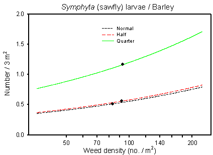
Fig. 6.1.
Model of the relationship between Symphyta larvae and weed
density. The centroid of the curve, corresponding to the mean weed density, is
indicated (· ). Notice that the model graphs do not show the
range of variation and that the log-based densities are not comparable with normal
arithmetic mean densities.
In wheat five of nine groups were positive correlated with increasing weed diversity/density. In beets, separate slopes models were analysed, but significant results were obtained only for one group. A correlation was found between Chrysomelidae (leaf beetle) adults and weed density, for which a positive connection was found at normal dosage (p=0.0363*), but a negative correlation was revealed in quarter dosage (p=0.0002***) (Table 6.3). A possible explanation could be that weed hoeing influenced the beetles negatively. Weed hoeing is a kind of unknown factor, which through disturbance and altered microclimate may have a negative impact on the arthropods in the plots that received reduced dosages of pesticides.
Table 6.3.
Schematic summary of the combined analysis of arthropod densities. Covariates
describing the abundance of weeds and differences in insecticide spraying intensity were
included in the analyses. Factors not included in any of the models have been omitted from
the table. S-Weeds: Weed diversity; Weeddens: Weed density. Statistical significance is
indicated as follows: */+/–: 0.01<p<0.05, **/++/– –:
0.001<p<0.01, ***/+++/– – –: p<0.001. +/– indicates if the
correlation is positive/negative. Abbreviations: Img.= Imagines Lar.=
Larvae, Nym.= Nymphs.
In some cases the covariates weed species richness and weed density (Table 6.3) eliminated the effect of the class factor dosage found in the analyses described in Table 3.5 – 3.7, indicating that the dosage effect found in chapter 3 may have been caused by an altered weed diversity/density. In barley, this was the case for Lepidoptera (p=0.0008***), which was positively correlated with species richness (Fig. 6.2). Since weed species richness and weed density are significantly correlated it may be random which of those that appears significant. The highly significant correlation, however, between Lepidoptera larvae and weed diversity without any correlation to weed density, is a major indication that the larvae mainly benefited from of a complex weed plant community created by reduced herbicide spraying.
The inclusion of the covariate weed density (significant at p=0.0002***) in the analysis of Miridae adults in barley (Fig. 6.3) resulted in a significant effect of dosage in contrast to the analysis in chapter 3. This indicated an improved model revealing an effect of both the weed community as well as a direct effect of pesticide application, the latter supported by a significant negative correlation with the parameter treatment intensity index of insecticides. In wheat, the addition of the significant covariate weed density made the class variable dosage become insignificant for Miridae imagines (Fig. 6.3), indicating that the dosage effect found in chapter 3 probably was caused by an altered weed vegetation.
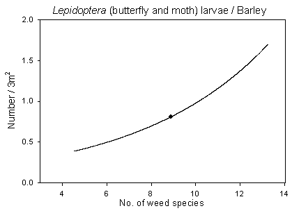
Fig. 6.2.
Models of the relationship between Lepidoptera and weed
diversity. The weed covariate replaced dosage (see Tables 3.8 and 6.2) as
significant factor in the analyses of the occurrence of arthropods in relation to
vegetation. The centroid of the curves, corresponding to the mean weed density, is
indicated (· ). Notice that the model graph does not show the
range of variation and that the log-based densities are not comparable with normal
arithmetic mean densities.
Another interesting result was that numbers of Curculionidae (weevils) both in barley and wheat were positive correlated with weed density (Fig 6.4). Neither in barley or wheat there were significant effect of dosage, but in wheat there was a negative correlation to the treatment intensity index of insecticides indicating some sensitivity to the insecticides.
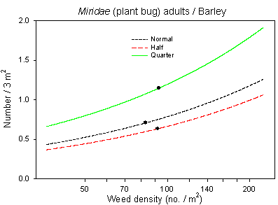
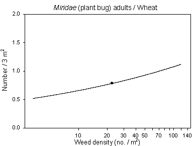
Fig. 6.3.
Models of the relationship between Miridae adults and weed
density in barley and wheat. The centroid of the curves, corresponding to the
mean weed density, is indicated (· ). Notice that the model
graphs do not show the range of variation and that the log-based densities are not
comparable with normal arithmetic mean densities.
Overall, specific arthropods seemed to benefit from a more complex weed vegetation in the cereals, especially in barley. In beets, no general trend could be revealed. The sometimes contradictory results, however, indicate that the findings should to be treated with caution.
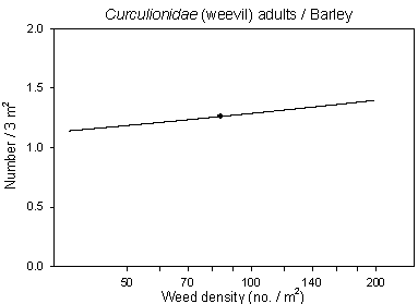
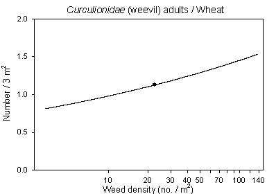
Fig. 6.4.
Models of the relationship of Curculionidae adults versus
weed density in barley and wheat. The centroid of the curves, corresponding to the mean
weed density, is indicated (· ). Notice that the model graphs
do not show the range of variation and that the log-based densities are not comparable
with normal arithmetic mean densities.
According to Potts (1986) there exists an association between the Miridae and the density of grass weed in the cereal crop. The situation is similar for some Cicadellidae and Delphacidae. These arthropods are common in the suction samples in all three crops in this experiment, but grass weed was not common and corresponding correlations were not obtained when analysed (not presented).
Hymenoptera, Syrphidae and Lepidoptera adults are known to collect nectar and pollen from flowering broad-leaved plants. The density of flowering species is known to be a limiting factor for these insects (Altieri & Whitcomb 1979). The number of flowering plants and species, which are mutually correlated, did improve in the cereals under a reduced pesticide regime (section 2.2.2.4), which again may have benefited the insect populations. In order to elucidate and quantify such an inter-trophic effect, the number of adults of Hymenoptera, Syrphidae and Lepidoptera were analysed in respect of the density of flowering plants and no. of flowering species per plot (1998 and 1999 only). No significant findings, however, were found for hymenopterans as a group (dominated by a range of ichneumonid wasps). A reason could be that the heterogeneity of the group made it difficult to detect specific trophic interactions. Looking at hymenoptera sub-groups, a significant positive correlation was found between adult Symphyta and the density of flowering plants in barley, but the estimated sawfly population was probably too low for a reliable analysis (not presented). No significant correlations were found for Syrphidae, but a significant positive correlation was found between Lepidoptera and the number of flowering broad-leaved plants in beets (p=0.014*) (Fig 6.5) and the number of flowering species (p=0.006**) (not illustrated). There was a tendency towards a corresponding correlation in barley (0.05<p<0.10) but not in wheat.
The highest density of adult Lepidoptera was observed in beets followed by barley and wheat and the strength of the correlations found followed the same pattern. The densities obtained of the flying species were probably underestimated due to their ability to escape during sampling and the elatively low estimated densities of the target species have most likely affected the results obtained.
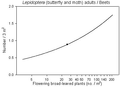
Fig. 6.5.
Model of the relationship of Lepidoptera adults versus the
density of flowering weed plants in beets. The centroid of the curve, corresponding to the
mean weed density, is indicated (· ). Notice that the model
graph does not show the range of variation and that the log-based densities are not
comparable with normal arithmetic mean densities.
6.2.2 Breeding season bird counts
The results of significance testing in the analyses of covariance are summarized in Table 6.4. The explanatory power of all models is good, with 69 to 76 percent of the total variation being explained. All main factors have significant effects on the distribution of at least two of the species tested, although the effects of dosage and crop may vary between farms. Block factors farm and field account for the major part of the variation (although the effect of farm may appear non-significant because it is tested against MS(Field(Farm))). In all models except one, the inclusion of a covariate increases the significance of the model; the covariate concerned is consistent within each species but differs between species.
Table 6.4.
Schematic summary of the analyses of mean numbers of Skylarks, Whitethroats
and small seed-eaters recorded on the fields 16 June - 5 August. Covariates describing the
abundance of weeds and arthropods were included in the analyses. Factors not included in
any of the models have been omitted from the table. Statistical significance is indicated
as follows: *: 0.01<p<0.05, **: 0.001<p<0.01, ***: p<0.001.
|
Skylark |
Whitethroat (field) |
Small seed-eaters (field) |
|||
|
Morning |
Afternoon |
Morning |
Afternoon |
Morning |
Afternoon |
Dosage |
|
(*)1) |
*** |
(*)2) |
*** |
|
Crop |
* |
** |
|
|
|
|
Year |
** |
|
|
|
*** |
*** |
Farm |
** |
** |
* |
|
** |
|
Field(Farm) |
*** |
*** |
*** |
*** |
*** |
*** |
Crop´ Farm |
|
|
*** |
** |
|
*** |
Dosage´ Farm |
|
|
|
* |
|
* |
Totaldrw (Crop) |
|
|
*** |
*** |
|
|
S_Weeds (Crop) |
** |
*** |
|
|
|
|
Weeddens (Crop) |
|
|
|
|
*** |
|
1)
Eliminated at p=0.0512) F=4.35, p=0.052 when tested against MS(Dosage´ Farm) 1) Eliminated at p=0.051
2) F=4.35, p=0.052 when tested against MS(Dosage´ Farm)
In the Skylark, numbers during the second half of the breeding season differ between crops, with the highest densities occurring in barley fields and the lowest densities in wheat (cf. Fig. 4.3). Before inclusion of covariates, these crop differences are significant on the morning counts (p = 0.037*), but not on the afternoon counts. Significant differences between dosages exist on the afternoon counts (p = 0.015*), but not on the morning counts, with higher densities being recorded in half- and quarter-dosage plots than in plots treated with normal dosage.
The analyses of covariance show that the significance of the Skylark models may be improved by including weed species richness in the models. The effect of weed diversity on Skylark numbers is only significant in barley fields (p = 0.0004*** and p < 0.0001*** on morning and afternoon counts, respectively) where Skylark densities increase with increasing weed species richness (Fig. 6.6 A). For the morning counts, a partitioning of the sums of squares before and after the inclusion of the covariate shows that the proportion of variance explained by the farm factor is reduced when the covariate is added to the model, indicating that it is mainly (part of) the variation between farms which is explained by the inclusion of weed diversity in the model.
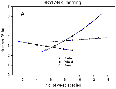
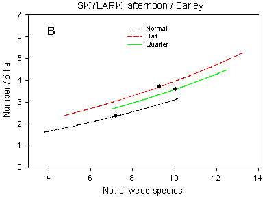
Fig. 6.6.
Models of the relationship between Skylark densities and weed species
richness for different crops (A) and dosages (B). A is based on the morning counts, B on
the afternoon counts. In A, notice that the slope of the curve is not significantly
different from zero in wheat and beets and that values for weed species richness in beets
are not directly comparable with those in cereals. In B, the relationship is shown for
barley fields only; the centroid of each curve, corresponding to mean weed species
richness at each dosage, is indicated (· ). Notice that the
model graphs do not show the range of variation and that the log-based densities are not
comparable with normal arithmetic mean densities.
A similar partitioning of the sums of squares for the afternoon counts indicates that not only the relative importance of the farm factor, but also the importance of differences in dosage is reduced when weed diversity is added to the model. Thus, part of the between-dosages variation in Skylark numbers may be ascribable to differences in weed species richness. Skylark densities and weed diversity are positively correlated (Fig. 6.6 B); the regression coefficients describing the shape of the relationship do not differ significantly between dosages (p > 0.10 in all pairwise comparisons). As indicated in the figure, weed diversity in barley fields decreases with increasing dosage (cf. section 2.2.2.2); consequently, the estimated mean densities of Skylarks are higher at quarter and half dosage than at normal dosage. On the afternoon counts, the highest Skylark densities are found in half-dosage plots; the reason for this is discussed in chapter 4.
The number of Whitethroats occurring in the fields differs between years, crops and dosages. After 15 June more birds are recorded in wheat and beet fields that in barley fields (cf. Fig. 4.4), although the crop differences are barely significant due to large variation between farms (p = 0.085 and 0.049* on morning and afternoon counts, respectively). Dosage effects are highly significant on the morning counts (p < 0.0001***), with higher numbers occurring at quarter and half dosage than at normal dosage, whereas the effect is less clear on the afternoon counts (p = 0.030*) due to large between-farms variation. Year-to-year differences are highly significant (p = 0.0005*** and 0.0020** on morning and afternoon counts, respectively) with higher Whitethroat densities occurring in the fields in 1998 and 1999 than in 1997.
The models for the morning and afternoon counts may both be improved by adding total arthropod dry mass (Totaldrw) as a covariate (Table 6.4). Whitethroat densities in all crops rise with increasing arthropod biomass (Fig. 6.7 A), although the effect is only significant in wheat (p = 0.072 and 0.017* on morning and afternoon counts, respectively) and beets (p = 0.0003*** and 0.0056**). In both models, a partitioning of the sums of squares before and after the inclusion of the covariate shows that the effect of the year factor is almost eliminated when Totaldrw is added to the model, indicating that year-to-year differences in Whitethroat densities in the fields may be caused by variations in the amount of arthropods available there. This interpretation is corroborated by an analysis of variance of Whitethroat densities in the border vegetation outside the fields which shows no clear between-years differences in Whitethroat numbers (p = 0.16).
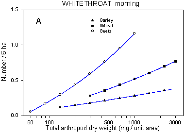
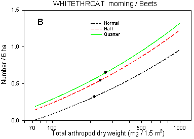
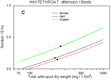
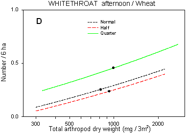
Fig. 6.7.
Models of the relationship between Whitethroat densities and total dry weight
of arthropods. A & B are based on the morning counts, C & D on the afternoon
counts. In A, the relationship is shown for different crops; the slope of the curve is not
significantly different from zero in barley and barely significant in wheat. Notice that
the values for arthropod dry weight in beets are not directly comparable with those in
cereals. B-D shows the relationship for different dosages in beets (B & C) and wheat
(D); the centroid of each curve, corresponding to mean total arthropod dry weight at each
dosage, is indicated (· ). In B, the curves for half and
quarter dosage are not significantly different; in C & D, the curves for normal and
half dosage are not significantly different. Notice that the model graphs do not show the
range of variation and that the log-based densities are not comparable with normal
arithmetic mean densities.
Further consideration of the sums of squares shows that the addition of Totaldrw to the models also reduces the relative importance of field and dosage differences, although not strongly so. Significant differences between dosages still exist after the inclusion of the covariate (p = 0.0003*** and 0.052 for morning and afternoon counts, respectively), indicating that just a minor part of the between-dosages variation in Whitethroat numbers may be explained by differences in arthropod availability. In all crops, the shape of the curve describing the relationship between Whitethroat densities and Totaldrw (Fig. 6.7 B-D) does not differ significantly between dosages (p > 0.40 in all pairwise comparisons of regression coefficients). As to the estimated densities of Whitethroats in half-dosage plots, the difference between morning and afternoon counts is complementary to the difference found in Skylarks and is discussed in chapter 4.
In the model without covariates, the numbers of small seed-eaters recorded on the morning counts differ significantly between crops (p < 0.0001***), dosages (p = 0.0073**), and years (p = 0.0031**). After mid-June, the highest seed-eater densities occur in beets and the lowest in barley, and densities are higher in plots treated with half and quarter dosage than in normal-dosage plots (cf. Fig. 4.5). On the afternoon counts, similar crop and dosage differences are indicated but are non-significant, partly due to large variation between farms.
The analyses of covariance show that the model for the morning counts may be improved by including weed density as a covariate. In all crops, seed-eater densities prove negatively related to weed density; the effect of weed density is significant in wheat (p = 0.0002***) and beets (p = 0.041*). In the model for the afternoon counts, no covariates are significant at the 5% level; S_Weeds (number of weed species) comes closest (p = 0.069).
The negative correlation between weed density and seed-eater numbers on the morning counts is inexplicable and, at least on the face of it, illogical. A partitioning of the sums of squares before and after the inclusion of the covariate shows that the proportion of variance explained by the field factor is reduced when the covariate is added to the model, whereas the proportion of variance explained by the dosage (and year) factors is increased. Thus, the variation in seed-eater numbers between dosages and years is not in any way related to differences in weed densities. Probably, the small seed-eaters accidentally occur at their highest densities in fields with low weed densities, without any causal connection. The lack of obvious concordance between the models for the morning and afternoon counts supports this conclusion.
Although treated as a group here, the different species of small seed-eaters vary in their habitat requirements and feeding behaviour. They are in various degrees associated with farm buildings and gardens, and the distance to these structures may be an important distributing factor. Also, the proportion of diet made up by animal food items varies between species. Whereas the cardueline finches are granivorous throughout the year, arthropods constitute an important part of the summer diet in species like Yellowhammer and Chaffinch, and the young of these species are almost exclusively fed animal food items (Cramp & Simmons 1977-94). These differences may be another reason why the analyses of covariance do not reveal any "sensible" relationships. Unfortunately, data on the individual species are too sparse and their distribution too far from normal to allow separate analyses.
As discussed above, the analysis and interpretation of the distribution of small seed-eaters imply some particular problems, but the appearance of a rather improbable result as highly significant in the analyses nonetheless calls for circumspection. Multiple regression and related techniques are powerful tools, and whenever a posteriori variable selection is involved (like here), the hypotheses tested are to some extent created by the data, and the risk of spurious correlations emerging as significant always exists. Therefore, even if the ancova results for Skylark and Whitethroat seem more credible than those for seed-eaters, they should be treated with caution as well.
6.2.3 Autumn bird counts
The addition of covariates to the models of the distribution of birds on the stubble fields did not in any case improve the models (in terms of a reduction of the model p value). When included, no variables describing cereal grain or weed seed abundance had any significant effect on the occurrence of any of the analysed species (p > 0.10 in all tests for b cov = 0). Only the factors indicated in Table 4.9 appeared as significant in the analyses, implying that neither differences in pesticide dosage nor differences in seed abundance (within the range found in this study) affect the autumn distribution of Skylarks, Meadow Pipits and small seed-eaters significantly. The separate analysis of Yellowhammer occurrence did not reveal any new information.