Technical Documentation of PestSurf, a Model describing Fate and Transport of Pesticides in Surface Water for Danish Conditions
2 New process Descriptions
- 2.1 Wind drift
- 2.2 Deposition of soil surfaces
- 2.3 Dry deposition
- 2.4 Colloid transport
- 2.5 Transport and transmission process in the streams and ponds
- 2.5.1 Sedimentation and resuspension
- 2.5.2 Diffusive exchange between water column and sediment in the rivers
- 2.5.3 Diffusive exchange between water column and sediment in ponds
- 2.5.4 Sorption to particles in water column and sediment
- 2.5.5 Sorption to macrophytes
- 2.5.6 Biodegradation of active substances
- 2.5.7 Photolytic degradation of active substances
- 2.5.8 Hydrolysis
- 2.5.9 Evaporation
In comparison to the standard-version of the MIKE SHE and MIKE 11 models, different components have been added. Some of these are added as pre-processing of data, while some are added directly into the model processes. The calculations performed and the formulas used, are described in the sub-sections of this chapter.
The new components are:
- wind drift (Asman et al., 2003)
- dry deposition (Asman et al., 2003)
- Deposition on the soil surface (Jensen and Spliid, 2003)
- colloid transport (Holm et al., 2003)
- pesticide-related processes in the river (described in this report, but based on work of Helweg et al., 2003)
2.1 Wind drift
The considerations, on which the choice of description is made, are described in Asman et al. (2003). Drift is described for agricultural crops, fruit trees and spruce trees.
For agricultural crops, the values of the Ganzelmeier-kurve (ref) corresponding to 95% drift is selected to represent average drift conditions for Denmark. Apple trees represent fruit trees. Spruce trees, when small, are sprayed from above, and the drift is therefore considered similar to agricultural crops. When the trees are larger, they are sprayed from the side, and to mimic this situation, the drift value is calculated as the average of drift for late and early hops. The values, on which the drift calculations are based, are given in Table 2.2.
Curves were fitted to each dataset. The relationships are
For agricultural crops:
Y = exp(ln(B) +β*x – x*A*e(α*x)) (Eq. 1)
where
x = distance
y = Drift as % of dosage
and the constants are give below:
| X<7.5 m | x>=7.5 m | |
| B | 25.6979 | 1.6195 |
| A | 2.7528 | 0.6745 |
| β | -0.4831 | 0.4709 |
| α | -0.6020 | -0.0061 |
The relationship allows x = 0, and fitted better than simpler relationships investigated.
For apples:
Y = B * Eax (Eq. 2)
Before leaves occur (before 1st of June)
if x<15, a=-0.127 and b = 39, else a=-0.102 and b = 31
After leaves has occurred, (after 1st of June)
if x <10, a = -0.1966 and b = 28; else 1= -0.0996 and b=11
For spruce:
Y = (29.35*exp(-3.07*log(x)) + 19.66 * exp(-3.56*log(x)))/2 (Eq. 3)
equal to the average of the fittings of early and late hops.
Figures showing measured data and fitted curves are shown in Appendix A.
The distance, x, is expected to consist of a distance from the sprayer to the stream, the buffer zone and half the width of the stream. The width of the stream is, in average, 1.3 m for Odder Bæk and 40 cm for Lillebæk. Half the width of the stream is therefore 0.65 and 0.2 m, respectively.
Table 2.1. The distance from the sprayer to the centre of the stream.
Tabel 2.1. Afstanden fra sprøjtedyssen til centeret af vandløbet.
| Crop | Distance from sprayer to stream | Buffer zone | Half river width |
| Agricultural crops | 0.0 m | 0-50 m | 0.2 or 0.65 m |
| Apple trees | 3.0 m | 0-50 m | 0.2 or 0.65 m |
| Spruce trees (sideways) | 1.5 m | 0-50 m | 0.2 or 0.65 m |
Each of the streams are divided into five segments (Styczen et al., 2004b, p. 43), and drift is calculated for each of these segments, taking into account the width of the buffer zone for each segment (For the pond, only one calculation is made). The amount is then recalculated to mass per stream segment, assumed to be sprayed into the river over 30 minutes. The resulting time series form direct input to the river model. For each spraying event, the drift from the whole length of stream is added over the same 30 minutes.
The implicit assumption is that the wind is always perpendicular to the stream, and blowing with a constant velocity. However, spray drift is added from one side of the water body only.
Table 2.2. Drift values, on which the drift calculations (equation 1-3) are based. The data are from BBA (2000)
Tabel 2.2. De vinddrift-værdier, der er basis for de udledte ligninger (ligning 1-3). Data stammer fra BBA (2000)
| Dist, m | Deposition, % of appl. Dose Agricultural crops |
Apples | Vines | ||
| Early stages | Late stages | Early | Late | ||
| 1 | 3.51 | ||||
| 2 | 1.24 | ||||
| 3 | 0.98 | 29.6 | 15.5 | 3.6 | 6.78 |
| 4 | 0.94 | ||||
| 5 | 0.75 | 19.5 | 10.1 | 1.63 | 3.43 |
| 7.5 | 0.42 | 14.1 | 6.4 | 0.87 | 2 |
| 10 | 0.33 | 10.6 | 4.4 | 0.55 | 1.36 |
| 15 | 0.2 | 6.2 | 2.5 | 0.29 | 0.79 |
| 20 | 0.12 | 4.2 | 1.4 | 0.19 | 0.54 |
| 30 | 0.11 | 2 | 0.6 | ||
| 40 | 0.4 | ||||
| 50 | 0.2 | ||||
The process is executed as part of the data transformation that takes place when input data given by the user is transformed to model input, and may thus be considered pre-processing.
2.2 Deposition of soil surfaces
The theoretical works, on which the relationships are based, are described in Jensen and Spliid (2003). The deposition on the soil is estimated in two different ways, for the situation with and without a plant cover.
For early sprayings, the plant cover is set to zero. The dose only has to be corrected for losses due to drift and dry deposition.
The total mass of dry deposition and spray drift to the stream is calculated, and deducted from the total mass of active substance sprayed. The result is divided by the sprayed area to calculate a slightly reduced average dose.
When a crop cover (> 20) is present, the dose is corrected for wind drift losses, and the deposition on soils is calculated as the corrected dose times a fraction. The fraction depends on the crop and the crop stage. The values as function of crop and time are shown in Appendix A of Styczen et al. (2004b).
In this case, the dry deposition is calculated based on emission from leaves, and the dose hitting the ground should therefore not be corrected for this loss.
In the test cases carried out, the corrections for drift and dry deposition on the average dose is less than 1%.
The resulting dose to the ground is transformed into a time series file (Spraying_corr.T0), where the dosage is repeated every year at the specified date, or, if the user specifies that spraying during rain is not allowed, the spraying date is moved forward until the criteria is fulfilled. The time series file is applied to the agricultural area of the catchment. This area is described by the file "Catchmentname_stream/pond_agrl0.T0" or "Catchmentname_stream/pond_agrl35.T0, depending on whether the buffer zone is below or above 35 meters.
The process is executed as part of the data transformation that takes place when input data given by the user is transformed to model input, and may thus be considered pre-processing. The names of the spraying file and the file describing the area to be sprayed are then transferred to the *.tsf-file (Catchmentname_stream/pond_pesticide/metabolite.tsf) that is part of the input to the MIKE SHE active substance simulation.
2.3 Dry deposition
The theoretical basis for the description of dry deposition is given in Asman et al. (2003). The description is a separate model entity, called PestDep, which is called by the pre-processing programme that transforms data from the interface.
In the model the wind direction (x direction) is always perpendicular to the water body (y direction). The deposition is assumed to be the same everywhere in the y direction along the river (in the model the river and the emission field are indefinitely long in this direction). The z direction is the vertical. The wind is always blowing from the emission area to the water body. Although this sounds unrealistic, it is in fact not so unrealistic because there are usually fields on both sides of the water body. Of cause the wind cannot blow pendicular to the entire length of a twisted and bended river. This was taken in to account through calculation of an effective exposed length of the river, calculated through projection of the river stretch on to straight line connecting the upper and lower end of the river (see Styczen et al., 2004b, section 4.2). Part of the time the wind will be blowing along the water body. This situation is not taken into account. In this way a maximum dry deposition to the water body is calculated.
The model version described here is made for streams and small ponds, not for large water bodies, such as seas.
In general, the programme is parameterised via the interface and the pre-processing programme. As for the drift calculations, time series are prepared for five segments of each river stretch. For the ponds, only one time series is prepared.
A number of parameters are given default values, or general values of relevance to the catchments. These are listed in Section 2.3.5.
2.3.1 Emission
The model distinguishes between emission from bare soil and a crop cover.
In the input file the indicator indicvol indicates the type of volatilisation calculation that has to be made:
- If indicvol = 1, the accumulated emission after application to crops during 7 days is calculated. In that case the parameters necessary for the calculation of the accumulated emission after application to normal moist fallow soil are read, but not used.
- If indicvol = 2, the accumulated emission after application to normal moist fallow soil during 21 days is calculated. In that case the parameters necessary for the calculation of the accumulated emission after application to crops are read, but not used. If the fraction of the active substance in the gas phase in the soil is outside the range for which the accumulated emission can be calculated a value of 0 is given (otherwise e.g. negative emissions will be generated).
The length of the emission zone in the x direction (downwind direction, perpendicular to the water body) is needed to calculate the absolute emission for the whole emission zone. It is calculated as: the 0.5*(total area of the catchment minus the area upstream of the upper end of each stream), divided by the length of the stream, measured as projections of the stream on to a straight line between the upper and lower end of the river (see Styczen et al., 2003b, section 4.2).
2.3.1.1 Emission from crops
Input data:
- Dose (kg active ingredient ha-1). To take into account that the compound may be non-neutral, the amount of neutral species is calculated using the pKa-value of the compound, assuming a pH of 7.
- Vapour pressure at a reference temperature (Pa).
- Reference temperature vapour pressure (K).
- Actual temperature of the crop (K). It is set to the actual air temperature that is read in the input file.
The dose and the vapour pressure comes from the interface while the reference temperature is assumed to be 20 C° (= 293.16 K). The actual temperature is read as the air temperature of the day that the spraying takes place.
Output data:
- Accumulated emission during 7 days (% of the dose).
The accumulated emission of active substances during 7 days after application to crops is calculated with the equation
10log(CV7)=1.528+0.466 10log(VP); for VP≤ 10.3 mPa (Eq. 4)
where:
CV7 = accumulated emission during 7 days after application (% of dosage of active ingredient).
VP = vapour pressure (mPa).
The vapour pressure is calculated for the actual temperature using equation
(Eq. 5)
where:
VP(T) = vapour pressure at temperature T (Pa)
VPref = vapour pressure at reference temperature Tref
Tref = reference temperature (K)
assuming a heat of evaporation of 95000 J mol-1. For some active substances the parameterisation of the accumulated emission from crops will lead to an emission of more than 100% of the dose. This is of course not correct. In that case the emission is set to 100%. This is not necessarily correct either, but should be used as a first guess and an indication that the accumulated emission is rather large.
2.3.1.2 Emission from normal moist fallow soil
Input data:
- Dose (kg active ingredient ha-1). Dose (kg active ingredient ha-1). To take into account that the compound may be non-neutral, the amount of neutral species is calculated using the pKa-value of the compound, assuming a pH of 7.
- Henry's law coefficient (cgas/cwater) at a reference temperature (dimensionless).
- Reference temperature Henry's law coefficient (K).
- Soil temperature (K).
- Dry bulk density soil (kg solid/m3 soil).
- Content of organic matter of the soil (%).
- Volumetric moisture content of the soil (%).
- Soil-liquid partitioning coefficient Kd (kg kg-1 solid/kg m-3 liquid).
The dose and Henry's law coefficient stem from the interface-information and are transformed as part of the pre-processing of data. Kd is calculated as the average value for the catchment (based on the average value of organic C or clay). The soil temperature, the dry bulk density, the content of organic matter, and the volumetric moisture content of the soil are parameters that are calculated on the basis of the conditions in the A-horizons of the catchment. For Lillebæk and Odder Bæk, the respective average bulk density is 1.42 and 1.32 g/cm3, and the respective average content of organic matter is 2.1 and 5.3%. With respect to temperature, a time series of air temperature is used, assuming that the topsoil has the same temperature as the air. As it is rather time consuming to extract the moisture content in every point in the catchment and average them for the calculations, the average moisture content at pF 2 was used as input for the calculations. For Odder Bæk the average moisture content at pF 2 is 0.376, while it is 0.269 in the Lillebæk scenario.
Output data:
- Accumulated emission during 21 days (% of the dose).
The accumulated emission of active substances during 21 days after application to normal moist fallow soil is calculated as:
CV21 =71.9+11.6 10log(100FPgas); for 6.3310-9<FPgas≤1
(Eq. 6)
where:
CV = accumulated emission during 21 days after application (% of dosage of active ingredient).
FP = fraction of the active substance in the gas phase in the soil.
The fraction of the active substance in the gas phase in the soil needed in this equation is calculated with Equations (7)-(16).
The following set of equations is necessary to find the fraction of the active substance in the gas phase (Smit et al., 1997).
The Henry's law coefficient gives the relation between the concentration of the active substance in the gas and water phase:
(Eq. 7)
where:
KH = Henry's law coefficient (dimensionless),
cgas = concentration of the active substance in the gas phase in the soil (kg active substance m3 air),
cliquid= concentration of the active substance in the water phase in the soil (kg active substance m-3 water).
Henry's law coefficient can be determined directly or can be determined from the molecular weight, vapour pressure and the solubility in water of the active substance. Both the measured or calculated values can be uncertain. It is not unusual that for one compound, Henry's law coefficients are reported in the literature differing an order of magnitude. Henry's law coefficient is rather temperature dependent.
The solid-liquid partitioning coefficient Kd gives the relation between the mass of active substance adsorbed to the soil particles and the concentration in the water phase in the soil. If a linear sorption isotherm is assumed Kd the following equation is found:
(Eq. 8)
where:
Kd= solid-liquid partitioning coefficient of the active substance (kg active substance kg-1 solid)/(kg active substance m-3 water).
X = mass of active substance adsorbed to the soil particles (kg active substance kg-1 solid).
Often the sorption is not linear and Kd is decreasing with increasing concentration in the water phase increases (Green and KaricKHoff, 1990). Kd is not very temperature dependent (Asmann et al (2003) refers to F. van den Berg, Alterra, Wageningen, personal communication, 2001).
The total concentration of active substance in the soil (in all phases) can now be described by:
![]()
(Eq. 9)
where:
csoil = concentration of active substance in the whole soil matrix (kg active substance m-3 soil) (Note: soil includes both the solid, water and gas phase of the soil),
θair = volume fraction of air in the soil (m3 air m-3 soil),
θwater = volume fraction of water in the soil (m3 water m-3 soil),
θsoil,dry = dry bulk density of the soil, i.e. soil without water, but including air (kg solid m-3 soil).
Equation (9) can also be written as:
![]()
(Eq. 10)
with the (dimensionless) capacity factor Q:
![]()
(Eq. 11)
The dimensionless fraction of the active substance in the gas phase is then:

(Eq. 12)
KH and Kd should be known, or can be derived from other properties of the active substance and/or the soil.
In this version of the model, water is derived from the MIKE SHE-calculation for the time of spraying. air is usually not given, but have to be derived from the following parameters:
- corg = organic matter content of the solid part of the soil (% of the volume).
- ρsoil, mineral = density of the mineral part of the solid phase of the soil (kg m-3). A constant value of 2660 kg m-3 is chosen (F. van den Berg, Alterra, Wageningen, personal communication, 2001).
- ρsoil,org = density of the organic matter part of the solid phase of the soil (kg m-3). A constant value of 1470 kg m-3 is chosen (F. van den Berg, Alterra, Wageningen, personal communication, 2001).
- ρsoil,dry = dry bulk density of the soil (without water, but including air) (kg m-3),
- ρair = density of air (kg m-3). A value of 1.25 kg m-3 is taken, which is representative of a pressure of 1 atmosphere and a temperature of 10°C,
- cmoist = volumetric moisture content of the soil (% of the volume).
Dry soil consists of organic matter and mineral parts. The density of the solid part of the soil ρsoil,solid (kg m-3) is calculated from the information on the organic matter content and the densities of the organic and mineral parts of the soil:
(Eq. 13)
As an intermediate step θair+water, the volume fraction of air and water together in the moist soil, can be found from:
(Eq. 14)
When deriving this equation one should note that the difference between dry soil and moist soil is that part of the volume fraction of air of the dry soil is replaced by water in the moist soil. This means that the volume fraction of air in the dry soil is equal to the volume fraction of air and water together in the moist soil.
The volume fraction of air air can then be found from:
![]()
(Eq. 15)
The Henry's law coefficient at the actual temperature is calculated with equation as
(Eq. 16)
where:
H = Henry's law coefficient (mol l-1 atm-1)
T = actual temperature (K)
Tref = reference temperature (K)
Rg = gas constant (8.314 Pa m3 K-1 mol-1 = 8.314 J K-1 mol-1);
δHA = heat of dissolution at constant temperature and pressure (J mol-1); A default value of –(95000 – 27000) = -68000 J mol-1 is used in PESTDEP if no values are known, and assuming a heat of dissolution at constant temperature and pressure of –68000 J mol-1. The parameterisation of the accumulated emission from normal to moist soil has a maximum of 95.1%.
2.3.2 Dry deposition
In the model there are 3 zones:
- Emission zone
- Non-spray zone
- Water body
In an emission zone no dry deposition occurs. In the model the dry deposition velocity in the non-spray zone is set to zero. This is done for two reasons. The first reason is that no information is available on the dry deposition of active substances to vegetation. The second reason is that in this way the maximum dry deposition to the water body will be estimated.
The flux to the water body is calculated assuming that the concentration of the active substance in the water body is zero. This is done, because normally the concentration in the water body will be highly variable in time and often been unknown during the emission periods (water bodies are not often sampled). In that way a maximum dry deposition is obtained. The following input and output data are used for the dry deposition velocity:
Input data:
- Friction velocity (m s-1).
- Henry's law coefficient (cgas/cwater) at a reference temperature (dimensionless).
- Reference temperature Henry's law coefficient (K).
- Actual temperature of the water body (K).
- Molecular weight of active substance (g mol-1).
- Average depth water body (m).
- Width of the non-spray zone in the x direction (downwind direction).
- Width of the water body in the x direction (downwind direction).
- Length of the water body (y direction, perpendicular to the wind direction) (m)
- Average aeration coefficient (day-1). This coefficient is calculated by DHI Water & Environment using the hydraulic MIKE 11 model that uses the Thyssen and Erlandsen parameterization (Equation 21).
The laminar boundary layer resistance (for rivers and lakes) is found from:
(Eq. 17)
where
u* = friction velocity (m s-1); this is a measure of turbulence. The larger u*, the larger the turbulence, and the larger the wind speed, and
(Eq. 18)
where:
νa = kinematic viscosity of the air (m2 s-1);
Dg = diffusivity of the gas in the gas phase (m2 s-1);
The surface resistance for rivers is found from Equations (19), (20) and (21) for rivers

(Eq. 19)
where:
KH = Henry's law coefficient (dimensionless); this is a measure of the solubility of the gas.
kw = aqueous phase mass transfer coefficient (m s-1); this is a measure of the transport velocity of the gas in water, which is a function of the mixing rate in the upper part of the water body.
kw is calculated as:
![]()
(Eq. 20)
where
Dw(gas) = diffusivity of the gas in water, m2s-1
dw = average depth of water, m
θ= temperature coefficient, 1.024 (dimensionless), and
![]()
(Eq. 21)
where
uw = average water velocity, m s-1
I = slope, m m-1
The calculation of K2d with Equation (21) takes place in MIKE 11 and data is extracted for the day of spraying.
For lakes, Equations (19), (22) and (23) are used:
An empirical relationship is used to describe the aqueous phase mass transfer coefficient for lakes, based on experimental data for 5 lakes (MacIntyre, 1995):
![]()
(Eq. 22)
where:
k(600) = the aqueous phase mass transfer coefficient of CO2 at 20°C in freshwater (m s-1)
k4 = constant necessary to obtain the right dimensions. Its value is 1.0 and its dimension is s1.6 m-1.6.
u(10) = wind speed at 10 m height (m s-1); the wind speed has usually measured on land near to the lake.
kw is calculated as:
(Eq. 23)
where
![]()
(Eq. 24)
and:
νw = kinematic viscosity of water (m2 s-1)
Dw = diffusivity of the gas in the water phase (m2 s-1)
In Equations (20) and (23), the diffusivity of the active substance in water is used, which is calculated from the molecular mass and corrected for the actual water temperature using Equations (25) and (26):
(Eq. 25)
In this equation
Dw,298.15 is in m2 s-1 and
MB is in g mol-1.
k4 = constant necessary to obtain the right dimensions. Its value is 1.0 and its dimension is ![]()
The diffusivity of the gaseous active substance Dsw(S,T) for (sea) water at temperature T (°K) and salinity S (pro mille) can be calculated from the following relation:
(Eq. 26)
where: ηw(0,298.15) is the viscosity of pure water at 298.15 °K and ηw(S,T) is the viscosity of (sea) water at salinity S and temperature T.
At last the dry deposition velocity is found from these resistances and Equations (27), (28) and (29):
The flux between the atmosphere and the surface is described by:
![]()
(Eq. 27)
where :
F = flux (kg m-2 s-1). The flux is here defined as negative when material is removed from the atmosphere.
Kg = overall gas phase mass transfer coefficient (m s-1)
cg,r = gas phase concentration at a reference height (kg m-3)
cg,surface = gas phase concentration that is in equilibrium with the concentration in the liquid phase (kg m-3). It is necessary that the concentration in the liquid phase (plant tissue, water) is expressed in a gas phase concentration, because only concentrations in the same phase can be compared.
Kg can be expressed as:
(Eq. 28)
where:
ra = aerodynamic resistance (s m-1)
rb = laminar boundary layer resistance (s m-1)
rc = surface resistance (s m-1)
In the model there is a resistance to transport in the air (ra, called "aerodynamic resistance") from a certain reference height to surface roughness length z0m, i.e. the height at which the wind speed is zero. It is the eddy diffusivity, the turbulence that is taking care of this transport. The aerodynamic resistance can be found by the following expression for ra neutral atmospheric conditions:
(Eq. 29)
where
κ= von Karman's constant (0.4; dimensionless)
The units in which ra is expressed is s m-1; this is just the inverse of a speed. In this equation zr is a reference height (m). In PESTDEP zr is the height of the centre of the lowest layer. The aerodynamic resistance is the same for all gases, i.e. it does not depend on the properties of the gas and depends only on the turbulence and the roughness of the surface for momentum.
Two combinations of surface roughness length (z0m) and friction velocity (u*) are used:
- For emission from crops: z0m = 0.1 m and u* = 0.386 m s-1.
- For emission from fallow soil: z0m = 0.01 m and u* = 0.284 m s-1.
These combinations are chosen in such a way that they give the average wind speed at 60 m height in Denmark. This average wind speed is calculated from the measured average wind speed at Kastrup Airport (near Copenhagen) for the period 1974-1983 at 10 m of 5.4 m s-1 using the l°Cal surface roughness length of 0.03 m.
The combinations of z0m and u* mentioned above are also used describe atmospheric diffusion.
Output data (not visible for the user; used as input to calculate the dry deposition):
- Dry deposition velocity (m s-1):
2.3.3 Atmospheric diffusion
Input data:
- Surface roughness length (m)
- Friction velocity (m s-1).
Output data (not visibile for the user):
- Wind speed as a function of height (m s-1) calculated with Equation (30).
(Eq. 30)
where:
u(z) = wind speed at height z (m s-1)
u* = friction velocity (m s-1); this is a measure of turbulence. The larger u* the larger the turbulence, the larger the wind speed.
κ= von Karman's constant (0.4; dimensionless)
z = height (m)
z0m = surface roughness length for momentum (m); this is a measure of the surface roughness, it is of the order of 1/10th of the height of obstacles.
- Vertical exchange (eddy diffusivity) (m2 s-1) calculated with Equation (31):
![]()
(Eq. 31)
where:
KHeat(z) = eddy diffusivity at height z (m2 s-1).
For a choice of values for the surface roughness length and the friction velocity see the previous section.
2.3.4 Integration of processes in the PESTDEP model
The PESTDEP model is a two-dimensional steady state K-model which integrates all above mentioned processes and is based on the following equation (Asman, 1998):
(Eq. 32)
where:
x = downwind distance (m).
z = height (m).
u(z) = wind speed at height z (m s-1).
cg(x,z) = concentration of the active substance in the gas phase (kg m-3).
KHeat(x,z) = eddy diffusivity (m2 s-1).
Q(x,z) = flux into the atmosphere (kg m-1 s-1). This is equal to the emission rate.
S(x,z) = flux out of the atmosphere (kg m-1 s-1). This is equal to the dry deposition rate.
2.3.5 Example of an input file
Table 2.3 Example of input file for the calculation of dry deposition, including explanation of the parameters and the source of information used in the model.
Tabel 2.3 Eksempel på inputfil til tørdepositionsberegningerne, med forklaring af de enkelte parametre og opgivelse af kilderne til informationen anvendt i modellen.
| Value | Name parameter | Meaning, units and what parameter is used for | Source |
| Bentazon | Namecomp | Name compound (40 characters) | |
| 5 | dose | Dose active ingredient (kg a.i. ha-1) | From user interface, modified according to the pKa-value so only the neutral fraction of the compound is used in the calculation. |
| 1 | indicvol | Indicator volatilisation
1= from crops, 2 = from soil |
Determined by the amount deposited on the ground. If more than 80 % is deposited on the ground, it is assumed that volatilisation takes place from the soil. Otherwise it takes place from the crop. |
| 1 | indicdep | Indicator deposition
1=stream, 2=lake |
From the choice of scenario in the user interface |
| 2.e-4 | Henrygref | Henry's law coefficient (cg/cw) at reference temperature (dimensionless)
[volatilisation from soil, surface resistance water] |
From the user interface |
| 293.15 | TkwHenrygref | Reference temperature Henry's law coefficient (K)
[volatilisation from soil, surface resistance water] |
20 C° is the assumed reference temperature |
| 1.e-4 | Vpref | Vapour pressure at reference temperature (Pa)
[volatilisation from crops] |
From the user interface. |
| 293.15 | TKVpref | Reference temperature vapour pressure (K)
[volatilisation from crops] |
20 C° is the assumed reference temperature |
| 283.15 | Tksoil | Actual temperature soil (K)
[volatilisation from soil] |
The air temperature at the time of spraying is used instead of the soil temperature (the volatilisation takes place from the upper few cm of soil. |
| 1400 | denssoil | Dry bulk density of the soil (kg solid/m3 soil)
[volatilisation from soil] |
The value represent the average of the conditions in the catchment. |
| 4.7 | orgmatpr°C | Content of organic matter of the soil material (%)
[volatilisation from the soil] |
The value represent the average of the conditions in the catchment. |
| 20 | moisturepr°C | Volumetric moisture content of the soil (%)
[volatilisation from soil] |
The value represent the average volumetric moisture content for the soils in the catchment at pF2. It is not extracted dynamically. |
| 2.4e-3 | Kd | Soil-liquid partitioning coefficient
(kg kg-1 solid)/(kg m-3 liquid) [volatilisation from soil] |
The value is calculated based on the percentage of organic matter given above. |
| 293.15 | Tka | Actual temperature air (K)
[laminar boundary layer resistance] |
The value is extracted from the time series file of air temperature. |
| 224.5 | molw | Molecular weight (g mol-1)
[laminar boundary layer resistance, surface resistance water body] |
From the user interface |
| 294.15 | Tkw | Temperature of the stream (K)
[surface resistance water body] |
The value is extracted from the time series file of water temperature. |
| 1.2 | depthw | Average depth water (m).
[surface resistance stream] |
Extracted from the MIKE 11 water simulations for the time of spraying. |
| 4.47 | k2_dhi | Average aeration coefficient stream calculated by DHI (day-1)
[surface resistance stream] |
Extracted from the MIKE 11 water simulations for the time of spraying. |
| 100 | dxemission | Upwind length of the emission area (m)
[concentration in the air] |
The length is calculated as half the average width of the catchment minus the buffer zone (see Styczen et al, 2003b, p 43) |
| 10 | dxns1 | Upwind length of the non-spray area before the water body (m)
[concentration in the air] |
The length of the non-spray area is either the naturally occurring buffer zone or the buffer zone set by the user, whichever is largest. It should be noted that the programme does not accept at width of 0, and a minimum value of 0.2 m is therefore used. |
| 5 | dxwater | Upwind length of the water body (m)
[concentration in the air] |
Extracted from the MIKE 11 water simulations for the time of spraying. |
| 5000 | dywater | Length of the water body perpendicular to the wind direction (m) | The stream is projected onto a line running through the catchment, and the projected length is used for the calculation. The streams are divided into 5 segments each. (see Styczen et al, 2003b, p 43) |
2.4 Colloid transport
The general Documentation for the module exists as part of Holm et al., (2003). The sections of relevance to PestSurf are copied below.
The incorporation of colloidal transport in the model includes description of the production of colloidal particles, the transport of these particles through the unsaturated zone, the saturated zone and drains. The module(s) presented herein have been developed for a specific project and therefore may lack some generality.
2.4.1 Generation of colloidal particles
A fundamental assumption is that colloids/particles are mobilised at the soil surface in response to rainfall. Mobilisation in deeper soil structures is assumed negligible compared to the mobilisation at the soil surface. The actual description of particle mobilisation is comparable to erosion modelling. The mobilisation of particles from a time-variant pool of potentially mobile soil particles at the surface is proportional to the kinetic energy of the rainwater and a parameter describing the ease with which, particles are detached from the particular soil-type.
Three approaches to modelling of colloid generation can be used:
- a kinetic energy model
- a raindrop momentum model
- A kinetic energy model similar to that of the MACRO-model (Jarvis and Larsson., 1998)
2.4.1.1 Kinetic Energy Model
Soil detachment by raindrop impact is described based on a kinetic energy model also used in the EUROSEM model by Morgan et al.1998c given by:
![]()
(Eq. 33)
where DET is the detachment (ML-2T-1)
KET is the total kinetic energy of the rainfall [MT-3],
k is an index of detachability of the soil [T2L-2] and
KH is a water depth factor [-].
The total kinetic energy of rainfall can be divided into energy by raindrop impact on the bare ground and energy from rain reaching the surface as leaf drainage:
![]()
(Eq. 34)
where KEDT is kinetic energy from direct throughfall [MT-3] and
KELD is kinetic energy from leaf drainage [MT-3].
The rainfall energy reaching the ground surface as direct throughfall is estimated as a function of rainfall intensity from an equation derived by Brandt 1989 relating energy to precipitation:
![]()
(Eq. 35)
where DT is direct throughfall [LT-1],
P is rainfall intensity [LT-1]
The energy of leaf drainage is estimated using the following relationship developed experimentally by Brandt (1989):
![]()
(Eq. 36)
where PH is effective plant height [L].
The model sets the kinetic energy by leaf drainage to zero when the height of the plant canopy is less than 14 cm in order to avoid the otherwise negative values predicted by Equation (36).
The water depth factor KH expresses a decrease in soil detachment with increasing water depth due to absorption of energy by the ponding water instead of the soil and a decrease in lateral water jets occurring within the splash crater. Several exponential and power functions have been proposed by Park et al. 1982, Hairsine and Rose 1991 and EUROSEM by Morgan et al. 1998c, of which three have been incorporated into this model.
The model by EUROSEM assumes an exponential relationship given by:
![]()
(Eq. 37)
where b is an experimentally derived coefficient [L-1].
The model by Parks relates the water depth factor to median drop size by:
![]()
(Eq. 38)
where dds is median drop size [L] and is computed by an empirical relation.
The water depth factor by Hairsine and Rose is similarly to Park's expression related to median drop size, however using a power function instead:
![]()
(Eq. 39)
The three models are depicted in Figure 2.1 below as a function of water depth and apart from the shape the curves are clearly very different. The function by EUROSEM decreases very steeply compared to the other two since no account for drop size is made in this formula.
Figure 2.1 Water depth factor functions calculated for a rainfall intensity of P=40 mm/h.
Figur 2.1 Vanddybde-faktor-funktioner beregnet for en nedbørsintensitet på 40 mm/h.
This kinetic energy model with the steepest of the above curves is used in the PestSurf scenarios.
2.4.1.2 Rainfall Momentum Model
The description of splash erosion using rainfall momentum is based on a model developed by Styczen and Høegh-Schmidt 1988. The method describes detachment of soil by the momentum of raindrops reaching the bare soil as well as by the momentum of drops falling from the canopy. The expression for soil detachment is given by:
![]()
(Eq. 40)
where A(e) is a soil resistance factor [T2M-1L-2],
MA is a mulch factor [-]
CM is the ratio of the total squared momentum of drops relative to the squared momentum of drops on bare soil [-]
MR is the squared momentum of drops on bare soil [m2T-3].
The resistance factor A(e) comprises the soil factors related to the resistance of the soil to erosion such as average energy required to detach one micro-aggregate and the probability that the detached aggregate retains energy for lifting to a water layer. The probability is assumed constant for all sizes of particles for a given soil and A(e) is thus a constant value. The mulch factor is the fraction of soil, which is covered by either mulch, stone and close growing vegetation and thus constitutes areas that are never reached by rainfall. This evidently implies that no erosion due to splash can occur here. The momentum of rainfall MR on bare soil depends on the drop size distribution of the rainfall. For rainfall following the Marshall Palmer distribution, the rainfall momentum is approximately proportional to the intensity of the rainfall lifted to a power given by:
(Eq. 41)
The canopy momentum factor CM is a factor expressing the relative effect of vegetation on soil detachment and is actual rain drop momentum from bare soil and vegetated soil given relative to rainfall momentum, i.e.
(Eq. 42)
where DH is the momentum of drops from the canopy [m2L-1T-2].
The momentum factor for canopy DH depends on drop velocity, which again depends on drop size and fall height. Vel°Cities have been measured by Epema and Riezeboes (1983) for various combinations of drop sizes and water heights and based on this set of data the following relationship is proposed for drop sizes between 4.5 – 6 mm:
![]()
(Eq. 43)
where the constants a, b, c and d are given in Table 2.4 below.
Table 2.4 Constants used in the calculation of splash erosion under plants
Tabel 2.4 Konstanter anvendt ved beregning af dråbeerosion under planter
| Drop sizes | (mm) | ||||
| Plant Height< 2 m | 4.5 | 5.0 | 5.5 | 6.0 | |
| a | - | - | - | - | |
| b | 0.7954 | 1.1058 | 1.4916 | 1.9601 | |
| c | - | - | - | - | |
| d | - | - | - | - | |
| 2-13 m | a | -0.5 | -0.5 | -0.5 | -0.5 |
| b | 1.2031 | 1.5930 | 2.0692 | 2.5496 | |
| c | -0.12416 | -0.15954 | -0.20184 | -0.23976 | |
| d | 4.33E-3 | 5.44E-3 | 6.70E-3 | 7.68E-3 | |
| > 13 m | a | 3.8647 | 5.4080 | 7.2934 | 9.5310 |
| b | - | - | - | - | |
| c | - | - | - | - | |
| d | - | - | - | - |
The water depth factor KH in Equation (40) was defined in Equations (37)-(39) and is identical to the formulation used in the kinetic energy model.
2.4.1.3 MACRO-Model
The original formulation of detachment in the MACRO model is given by:
![]()
(Eq. 44)
where DET is the particle detachment rate (ML-2 T-1)
Kd1 is an index of detachability of the soil [T2L-2]
Ms is the mass fraction of dispersible (movable) particles (g/g soil), and
KET is the kinetic energy from Equation (34).
The pool of detachable particle Ms is time-variant according to:
(Eq. 45)
where s is the soil bulk density (ML-3)
zi is the depth of top-soil influenced by detachment and dispersion (m) (L)
α is the share of the detached particles that are actually transported away from the soil surface (0≤α≤1)
Rrep is the rate of replenishment of the pool of particles (ML-2T-1)
The process of replenishment is not well known (or described) and therefore a simple functional relationship is used to describe the replenishment towards a maximum value Mmax (g/g soil):
(Eq. 46)
where kr is the replenishment rate coefficient (ML-2T-1)
The temporal development in the pool of dispersable particles is calculated by analytical integration of (45) leading to:
(Eq. 47)
2.4.1.4 Generation of boundary condition
The output from the subroutine for calculating detachment is 'DET' given in units of mass/area/time. The detachment is then automatically added to the overland component as a source and may pond, rate or run off on the surface.
2.4.2 Modification of Macropore Module for MIKE SHE
Simulations showed that it was necessary to perform an adjustment in the code of the Macropore Module for Mike She. The physical water exchange between macropores and matrix: S (see Equations (3) and (5) in manual for the Macropore Module) was only allowed to transport water from matrix to macropores and not to uptake water the macropores into the matrix. This means that when water enters the macropores, it only leaves the macropores again when reaching the saturated zone. This representation of macropores is the same as used in the DAISY model (Hansen et al., 1990).
2.4.3 Transport of colloids
Colloid transport is handled as transport of any other species in MSHE AD. Readers are referred to the manual for MSHE AD for further explanation of the principles applied in the transport algorithm. Apart from the general advective-dispersive transport, specific sink terms for filtration of colloidal particles will apply. Filtration of colloids in macropores is described by:
![]()
(Eq. 48)
where F is the filtering rate (M Ltot-3 T-1).
fmacro is the macropore filter coefficient (T-1)
Ccol is the colloid concentration in the aqueous phase (MLwater,macro-3)
θ macro is the water content in the macro pores (L3water /L3total)
For filtration of colloids in the matrix the same type of expression is used, but the filter coefficient is expected to be significantly higher.
2.4.4 Transport of active substance
The active substance (and its metabolite) can exist in three states (names in parenthesis indicate the name of the species in reactions listed in Figure 2.2, below):
- pesticide dissolved (PESTIC)
- pesticide adsorbed to colloids (PESTCOL)
- pesticide adsorbed to soil (PESTSOIL)
- metabolite dissolved (METABOL)
- metabolite adsorbed to colloids (METCOL)
- metabolite adsorbed to soil (METSOIL)
Each of these states is defined as a species in the setup for MIKE SHE AD. The distribution of the active substance and the metabolite between the three possible states; is handled by the Sorption-Degradation (SD) module of MSHE. The module also handles the degradation of the active substance and following formation of the metabolite. The exchange of solute between matrix and macropore is handled by the AD-module for macropore transport as for any other species (see manual for the Macropore Module of MIKE SHE, DHI).
Figure 2.2 List of reactions solved
Figur 2.2 Reaktioner, der løses I kolloid-modulet
2.4.5 Reactions accounted for in the solver
The reactions listed below are solved in four domains:
- unsaturated zone macropores
- unsaturated zone matrix
- saturated mobile zone
- saturated immobile zone
Each sorption reaction is defined as two reactions; a sorption and a desorption reaction. An equlibrium constant is specified and the correct proportion between the two rates is chosen from an arbitrary (high) forward rate and the relation Kd = kforward/kbackward. The filtration processes are only directed from the aqueous phase towards the solid phase. The filtration processes are defined so that:
- filtrated colloids become soil and can not be re-enter the aqueous phase as colloids (colloids are only generated on the soil surface)
- filtrated colloids carrying active substance or metabolite is converted to active substance/metabolite sorbed to soil, and hence the active substance can re-enter the aqueous solution
The degradation reactions are first-order reactions which can be made dependent upon water-content and temperature (see SD-manual).
The total system is solved using a L-stable Rosenbruck with embedded formula for error control.
2.4.6 Parameterisation used in PestSurf
Particle-facilitated transport is activated by:
- setting a logical COLLOID = TRUE at the bottom of the transport setup file (.tsf)
- specifying the input for the necessary input parameter for MSHE AD
- specifying the input for the activation module in a file named 'setupname'.colloid.
The specification of the logical 'COLLOID' is shown in Figure2.3 below.
Figure 2.3 Activation of colloid module at bottom of .tsf-file.
Figur 2.3 Aktivering af kolloid-modulet i bunden af .tsf-filen.
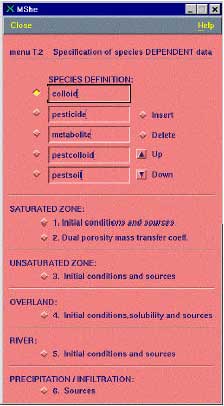
Figure 2.4 Input for MIKE SHE AD-module. This is only relevant if the module is used without the PestSurf interface
Figur 2.4. Input til MIKE SHEs AD-modul. Dette er kun relevant hvis modulet startes uden om PestSurf-brugerfladen
The species must be listed in the following order (see also Figure 2.4):
- colloid
- pesticide
- metabolite
- pestcolloid
- pestsoil (immobile)
- metcolloid
- metsoil (immobile)
Input for initial conditions, solubility and sources are given as usual, except that source-terms for colloids should be specified in the file 'setupname'.colloid. An example input file is shown in Figure 2.5. The meaning of the different input-parameters is explained below.
Figure 2.5 Example input file *.colloid
Figur 2.5 Eksempel på inputfil til kolloidberegningerne, *.colloid
Code for detachmentmodel: Refers to the three options for determing the detachment rates:
1: kinetic energy model
2: raindrop momentum model
3: MACRO-model
Waterdepth correction: exponential factor b in Equation (37)
Alpha: Coefficient (0≤α≤1), which determines the fraction of detached particles that infiltrate (See Equation (45)).
Parks/Rose/Eurosem: Determines which of the models to be used for calculating the water depth correction.
1: Parks
2: Rose
3: Eurosem
Soil type distrubution: Areal distribution of soil types. Can refer to .T2-file or be an integer number
No. of soil types: Number of different soil types in setup. Here two soil types are given, hence the soil data are repeated for each soil type.
Soil type code: Soil code used in the soil distribution file.
Detachability, Kd: Parameter Kd (T2L-2) in Equation (33). Erosion modelling gives a range of values from 2-10 kg/J for uncompacted soils and 8-44 kg/J for compacted soils (Morgan et al., 1998).
Soil resistance factor, A(e): Soil resistance factor A(e) (T2M-1L-3)in Equation (40) (Only relevant for detachment model 2)
Mulch factor, MA: Mulch factor MA (-) in Equation (40). (Only relevant for detachment model 2).
Replenishment rate, kr: Replenishment rate coefficient kr (M L-2 T-1) in Equation (46)
Dry bulk density, s: Dry bulk density of top soil s (ML-3) in Equation (46)
Influence depth, zi: Depth of top-soil influenced by detachment zi (L) in Equation (45)
Maximum detachable soil, Mmax: The maximum amount of detachable soil particles Mmax (g/s soil) in Equation (46)
Vegetation distribution: The distribution of vegetation in the model area is either specified with a single grid code value, if the same vegetation is present in the entire model area or by a .T2 map file containing a number of grid codes, each one representing a specific vegetation type. Each vegetation type is characterised by a number of different properties such as plant cover, plant height, angle and shape. The different plant properties are described in the following sections and must all be specified for each vegetation type.
No. of veg. types: The total number of plant types in the model is specified here. Here, two vegetation types are chosen and the vegetation data is repeated for each vegetation type.
Veg type code: The vegetation type code is an integer value representing a specific vegetation type, which is initially specified in the aforementioned map file.
Cover: The density of vegetation is expressed by the areal fraction of plant cover, which is dimensionless (0 < cover < 1). Can be given as a constant value or as a time series.
ICmax: ICmax is the maximum volume of interception by plant cover and is given as a water depth in [L]. Can be given as a constant value or as a time series.
Plant height: Effective plant height is used for computing the energy of leaf drainage in Equation (36) [L]. Can be given as a constant value or as a time series.
Plant angle: The plant angle is given in radii and is thus dimensionless.
Plant shape: Two different shapes of vegetation have been incorporated into the model. One type (1) represents grass or grass like vegetation and the other type (2) covers all other kinds of vegetation. The shape of the plants is of importance in computing stemflow. For grasses or vegetation with mean diameters smaller than the mean diameter of the drops, gravity plays an important role as opposed to other types of vegetation.
Canopy raindrop size: Canopy raindrop size is important in computing detachment by splash in relation to the computation of the water depth factor (L).
Stepmin: minimum time step used in the chemical solver
Stepmax: maximum time step used in the chemical solver
rtols: relative tolerance for the chemical solver
atols: absolute tolerance for the chemical solver
steps: the equilibrium reactions are solved as a set kinetic reactions with a forward and backward reaction. Steps specifies how much faster the slowest reaction rate for the equilibrium reactions is compared to the largest kinetic reaction rate. Large values will cause the equilibrium reactions to be more precisely described but could cause the solver to use smaller timesteps.
2.5 Transport and transmission process in the streams and ponds
The standard MIKE 11 AD (advection dispersion) module added on top of the standard MIKE 11 HD (hydrodynamic) module was used for description of the transport of active substances in the rivers caused by advection and dispersion. On top of the AD module a suite of process, which describes the sorption, biodegradation and other transport and transmissions process, was implemented in a dedicated MIKE 11 PE (pesticide) module. The following section gives a technical description of the process implemented in the pesticide module. A conceptual diagram of the process descriptions of the pesticide module appears from Figure 2.6.
Figure 2.6 Conceptual drawing of the MIKE 11 pesticide module
Figur 2.6 Konceptuel model af MIKE 11's pesticidmodul
2.5.1 Sedimentation and resuspension
processes for description of sedimentation and resuspension are implemented in the MIKE 11 pesticide module, but it was decided to set the exchange of sorbed active substances between the water column and the sediment to 0. For a further discussions thereof see Section 2.9 in Styczen et al. (2003a). Consequently a detailed description of the sedimentation and resuspension is not provided in the present report.
2.5.2 Diffusive exchange between water column and sediment in the rivers
In the river the sediment is supposed to be well mixed and a one-layer model of the sediment is therefore considered as appropriate. Under these assumption the diffusion from the water column in to the sediment is described by the following differential equations:
dCW/dt = D*AREA*(SW-CW)/(FZ*Volume),
(Eq. 49)
where
CW denotes the concentration of dissolved active substance in the water column
SW denotes the concentration of active substance in the pore water
FZ denotes the thickness of the laminar boundary layer
AREA denotes the area of the bottom
FZ denotes the thickness of the laminar boundary layer
D denotes the molecular diffusion coefficient
Volume denotes the volume of the water column
The diffusion from the pore water in to the water column is described by the following differential equation:
dSW/dt= D*AREA*(CW- SW)/(FZ*Volume),
(Eq. 50)
where
Volume denotes the volume of the pore water.
2.5.3 Diffusive exchange between water column and sediment in ponds
The sediment in the ponds is not assumed to be well mixed and diffusive process might therefore take place within the sediment. This diffusion, and the sorption and biodegradation of active substance is described by a module implemented in the AD scheme of the MIKE 11 model. A description and a testing of this module appear from Appendix E.
2.5.4 Sorption to particles in water column and sediment
Considering sorption as a reversible process the adsorption and desorption might be described as two opposite first order process (Nyffeler et al 1984) yielding the following differential equations:
dCW/dt = K2*CS - CW*K1
(Eq. 51)
and
dCS/dt = CW*K1 - K2*CS,
(Eq. 52)
where
CW denotes the concentration of active substance dissolved in water
CS denotes the concentration of active substance sorbed to particles
K1 denotes a (pseudo) first order adsorption rate
K2 denotes a first order desorption rate
The adsorption rate is in fact a pseudo first order rate constant, as described in experiment by Nyfeller et al. (1986) and expresses a linear relationship to the concentration of sorbing particles.
Or expressed mathematically:
K1 = K1**CP,
(Eq. 53)
where
K1* denotes the adsorption rate constant
CP denotes the concentration of particles in the water column or for the sediment the ratio between solid matter and water.
2.5.5 Sorption to macrophytes
The active substance in the water column might also sorb to macrophytes. As for the sorption to sediment particles and suspended matter the sorption to macrophytes was described by a first order sorption and a first order desorption rate. Hence the same basic equation as for sorption of active substances to particles was used except that the concentration of particles, CP, was substituted with the concentration of macrophytes.
2.5.6 Biodegradation of active substances
Dissolved active substances in the pore water and water column are assumed to undergo biodegradation. In every case the degradation will be formulated as a first order degradation yielding the differential Equations (54) and (55) for degradation of dissolved active substances in water and pore water respectively.
dCW/dt = Kcs*CW,
(Eq. 54)
where
CW denotes the concentration of dissolved active substance in the water column (g-pesticide/m3)
Kcw denotes a first order degradation rate for active substance dissolved in the water column(h-1)
dSW/dt = KsW*SW,
(Eq. 55)
where
SW denotes the concentration of active substance dissolved in the pore water (g-pesticide/m3)
KsW denotes a first order degradation rate for active substance dissolved in the pore water (h-1)
Biodegradation is influenced by temperature, where the rate increases with increasing temperature (Dickson et al, 1984). The temperature effect is usually presented by the Arrhenius-like Equation (57) as:
![]() ,
,
(Eq. 56)
where
T= water temperature (C)
To= reference temperature for which reaction rate is reported (C)
A = constant
At temperatures below 5°C, biodegradation is assumed to stop.
2.5.7 Photolytic degradation of active substances
As described in Section 2.14 of the calibration report (Styczen, 2004a) only the direct photolysis is accounted for by the MIKE 11 PE module. To calculate the photolytic degradation one needs to know the quantum yield defined as:
Click here to see the Equation.
Assuming that the amount of light absorbed by the chemicals is much less than the amount of light absorbed by the water body the light absorption of the compound per unit volume can be expressed as:
(Eq. 58)
where
Ia(λ) denotes the total number of quanta absorbed of the array of wavelength (λ)
W(λ) denotes the total light intensity at the surface distributed at the array of wavelength (λ)
ε(λ) denotes the decadic molar extinction coefficients distributed at the array of wavelength (λ) (mol quant m-1)
αD (λ) denotes the apparent or diffuse attenuation coefficients of river water distributed at the array of wavelength (λ)
Cd denotes the concentration of active substance
Depth denotes the depth of the river
Zmix depth of pond or river
α(λ) denotes the attenuation coefficients of river water distributed at the array of wavelength (λ)
When the total number of quanta absorbed, Ia(λ), and the reaction quantum yield, φr(λ), are known then a first order photolytic degradation rate, Kphoto, can be calculated as:
Kphoto = Ia(λ)*φr(λ),
(Eq. 59)
And the photolytic degradation can then be expressed by the differential equation:
dCW/dt = -Kphoto*CW,
(Eq. 60)
Generally, organic compounds including active substances should absorb light in the wavelength range of 290-600 nm in order to be photolytically transformed (Guenzi et al., 1974) and the light absorption spectra, ε(λ), for the active substance in this interval is available from the user interface. In addition is the reaction quantum yield φr(λ) (Schwarzenbach 1993) available from the user interface. On the contrary the remaining terms of Equation (6) have to be estimated on the basis of data from the catchments. Hence the attenuation coefficient, α(λ) have been set to 2.5 for all wavelength after the calibration exercise (Styczen et al 2004).
αD=α(λ)* D
(Eq. 61)
The diffuse or apparent attenuation coefficient is estimated on the basis of, α(λ), D(λ) and the equation of Neely and Blau (1985):
αD(λ) = α(λ)*D(λ),
(Eq. 62)
where
D(λ) denotes the ratio between the average path length and the depth for an array of wavelength (λ)
For both rivers D(λ) was set to 1.6 based on considerations of Neeley and Blau (1985), who stated that D(λ) is between 1.05 and 1.3 for blue and UV light in surface water and Schwarzenbach (1993), who stated that D() might be 2 in very turbid water. All though Equation (63) shows that the attenuation is a function of the wavelength it was assumed that α(λ) and αD(λ) is the same for all wavelengths (λ). This assumption was needed since the detailed chemical composition of the organic matter in the water not is known and the attenuation at different wavelength can therefore not be estimated.
2.5.8 Hydrolysis
The hydrolysis of organic chemicals in water is often observed as a first-order reaction given by (Thomann and Muller, 1987):
(Eq. 63)
where
KHT denotes the hydrolysis rate constant (h-1)
The hydrolysis rate constant (KHT) may include contributions from acid- and base-catalysed hydrolysis as well as nucleophilic attack by water (neutral hydrolysis). The following equation explains these possibilities explicitly:
![]()
(Eq. 64)
where:
KH denotes the acid catalysed hydrolysis rate constant (mol-1*h-1)
KOH denotes the base catalysed hydrolysis rates constant (mol-1*h-1)
KH2O denotes the neutral hydrolysis rates constant (h-1)
The acid, base and neutral hydrolysis constants are available from the user interface. [H+] and [OH-] was set to 7.5 and 6.5 respectively corresponding to the average measurements of pH conducted by the counties.
2.5.9 Evaporation
The evaporation of active substance from the water to the air is described by the same basic equation as for dry deposition outlined in Section 2.3.2. However, the MIKE 11 pesticide module calculates the evaporation for every time step of 3 minutes, whereas the model for dry deposition, PESTDEP, calculates the dry deposition to the river with a time resolution of one week. Due to the large differences in time resolution it is not relevant to link the two models dynamic. In the model the evaporation of active substances was therefore considered as independent from the dry deposition. As a consequence the concentrations of active substances in the air was set to 0 when the evaporation of active substances was calculated.
Version 1.0 Maj 2004, © Danish Environmental Protection Agency