Technical Documentation of PestSurf, a Model describing Fate and Transport of Pesticides in Surface Water for Danish Conditions
3 User Interface
- 3.1 How to start the system
- 3.2 The system
- 3.3 General Menu-pages
- 3.3.1 Basic parameters
- 3.3.2 Catchment and type of surface water
- 3.3.3 Crop
- 3.3.4 Width of protection zone
- 3.3.5 Spraying data
- 3.3.6 Basic chemical and physical properties of the active substance (and metabolite)
- 3.3.7 Sorption of active substance in soil
- 3.3.8 Degradation of active substance in soil
- 3.3.9 Sorption of active substance in surface water
- 3.3.10 Aerobic degradation of active substance in surface water
- 3.3.11 Anaerobic degradation of active substance in surface water
- 3.3.12 Hydrolysis of active substance in surface water
- 3.3.13 Photolysis of active substance in surface water
- 3.3.14 Pesticide transformations to metabolite
The user interface is a bridge between the user and the scenarios. It transforms the parameters specified in its menus to time series, maps and files that are used to run the model. Each menu page is described in the following, and this is followed by a description of the transformations taking place between the user interface and the model.
3.1 How to start the system
Start the Mike Zero shell, press File, New, and select MIKE SHE/Pesticide in Surface water, or select File, Open and the appropriate parameter file (*.psw), if a file already exists.
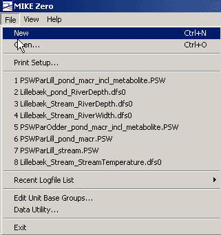
Figure 3.1 Opening a file in PestSurf.
Figur 3.1 Åbning af fil i PestSurf.
3.2 The system
The model system allows the user to simulate active substance (and one metabolite) on six different scenairos, that is
- Lillebæk stream
- Lillebæk macorphyte dominated pond
- Lillebæk phytoplankton dominated pond
- Odder Bæk stream
- Odder Bæk macorphyte dominated pond
- Odder Bæk phytoplankton dominated pond
For each of the scenarios, a set of water movement files exists for each crop allowed in the user interface (14 crops in total, 13 water files per scenario as spring barley and spring wheat utilizes the same file). The files are named "Catchment"_"waterbody"_crop, with an extension that specifies whether it is a MIKE SHE or a MIKE 11-flow-file. These files are stored on external disks due to their size. The right disk has to be selected for the particular run. The selected water movement file is the basis for the calculation of solute transport. The directories, where the files are l°Cated, are selected via "Settings", see Figure 3.2.

Figure 3.2 Setting of the location of MIKE SHE Water Movement files.
Figur 3.2 Specifikation af placeringen af MIKE SHE's vandberegningsfiler.
In order to carry out the solute calculations, input parameters have to be specified for wind drift (see Section 2.1), for the dry deposition model "PestDep" (see Section 2.3), and the MIKE SHE and MIKE 11 solute transport and transformation modules. The menus described in Section 3.3 are used for specifying the necessary parameters. All other parameters are pre-specified in templates, which are stored separately in the system.
The basic input files required for MIKE SHE and MIKE 11 are shown in Table 3.1. Templates for all the necessary files are prepared and stored in the system. There are eight of each file, as they exist for each scenario and with and without Metabolite. For each catchment the templates for the macrophyte and phytoplankton dominated ponds are identical.
Table 3.1 File types and short description of files required for MIKE SHE and MIKE 11 active substance calculations.
Tabel 3.1 Filtype og kort beskrivelse af filer til MIKE SHE og MIKE 11-pesticidsimuleringer.
| MIKSHE | |
| .tsf –files | General solute transport parameters |
| .xtsf-files | Specific sorption and degradation parameters |
| MIKE 11 | |
| .bnd11 | Boundaries and sources for matter and water |
| .ad11 | Parameters for advection and dispersion |
| .pe11 | Parameters for transport and transmission of active substances |
| pesticide_diffusion.txt | Parameters for diffusion, adsorption and decay of active substances in the sediment beds of the ponds. |
| .sim11 | Specification of files for boundaries, sources and parameters |
The name-convention for the files is "Catchment"_"waterbody"_Pest/PestMetab.extension.
Some of the values in the above files are given standard values. One of each template file for MIKE SHE is included in Appendix B, and one of each template file for MIKE 11 is included in Appendix C, with comments on the selected standard values. The standard values selected for the colloid module is included in Appendix B.
When the menu-pages, described in Section 3.3, are filled out, and before the simulations can start, the input given on the menu-pages are transformed to the values required for the models to operate. This is done by a pre-processing programme.
The pre-processing programme:
- selects the correct water movement file
- selects the correct template files for MIKE 11 and MIKE SHE
- Calculates wind drift for each section of the stream or the water body (Section 2.1)
- Calculates dry deposition for each section of the stream or the waterbody (Section 2.3)
- Transforms the values for drift and dry deposition into time series files for MIKE 11
- Calculates a time series files for calculation of photolysis rate in MIKE 11 on the basis of the daily global radiation and the absorption spectra of the active substance
- Corrects the dose on the agricultural land according to the calculated drift and deposition losses (Section 2.2)
- Recalculates input values in the appropriate form and modifies the template files for MIKE SHE/MIKE 11 with the revised values.
- Creates a new directory with the name of the run and stores a copy of all the modified templates and other produced files.
The directory is divided into MAPS, MIKE11, TIME, SIGNALS and temp. The user can therefore always check the actual input used. When the user has finished working with a simulation, the whole directory can be removed without damaging the programme. However, the user may wish to store the parameter file (.psw) and the MIKE 11 Result file that includes the results to be displayed in the result presentation programme, se Section 4.
Table 3.2 List of files moved to the working directory established by the User interface when a simulation is initiated. Some of these are generated by the programme.
Tabel 3.2 Filer, der flyttes til arbejdsfolderen, der genereres af brugerfladen når simuleringen starter. Nogle af filerne genereres af programmet.
| location | File Name | Explanation |
| Under main directory | InputDryDepositionCalculations.txt | All input for the dry deposition calculation |
| . colloid | Input to colloid calculations | |
| .tsf | Input to MIKE SHE Advection-Dispersion module | |
| .xtsf | Input to MIKE SHE sorption/degradation module | |
| Spraying.psf | Input to winddrift and selected input to dry deposition calculations | |
| W5.* | Results from the last calculation of the dry deposition programme. | |
| \MAPS | Kd | Calculated values of Kd |
| DT50 | Calculated values of half life | |
| Agrl | Map indicating area to be sprayed. | |
| Rhob | Bulk density files used | |
| \MIKE11 | RES11-files | The selected water movement files (with the name of the catchment and the
crop are moved to this directory.
The RES11-file with the name of the directory is the output file of the scenario. |
| Hd11, xns11 and nwk | Describes the basic river system and stream setup. | |
| Ad11 | Parameters for the advection/dispersion simulation of MIKE11 | |
| Bnd11 | Specification of boundary conditions for MIKE11 | |
| Pe11 | Specification of Pesticide parameters for MIKE11 | |
| Sim11 | Specification of the overall simulation with MIKE 11 | |
| Pesticide_update_frequency.txt | The file is generated by the user interface and guides the frequency of storing of MIKE 11-results 1. | |
| Pesticide_diffusion.txt | Specification of pesticide parameters for the sediment in ponds | |
| \TIME | CropCover.T0 | Input to colloid programme |
| CropHeight.T0 | Input to colloid programme | |
| Crop Interception.T0 | Input to colloid programme | |
| SoilDeposit.dfs0 | Specifies the fraction of the pesticide depositing on the ground as a function of date. | |
| Deposition_stream_spray.dfs0 | Time series specifying the additions from spray drift and dry deposition on the different segments of the stream or pond | |
| _RiverDepth.dfs0 | Time series of variation in water body depth | |
| RiverWidth.dfs0 | Time series of variation in water body width | |
| Streamtemperature.dfs0 | Time series containing the temperature of the water body | |
| _prec.T0 | Time series of the precipitation | |
| _trd.T0 | Time seris of the air temperature | |
| Photolysis.dfs0 | Timeseries calculated on the basis of the light absorption spectra of the compound, the spectral composition of the sunlight and the daily global radiation. The timeserie is used for calculation of photolysis. | |
| Spraying_corr.T0 | The dosage sprayed on the fields (MIKE SHE) | |
| biomass.dfs0 | Timeseries of the biomass of macrophytes in ponds and streams. | |
| \SIGNALS | Contains log-files and error-messages from MIKE SHE, generated during the run | |
| \tmp | Temporary files of no interest. |
In addition to the above files, a number of support-files are used, either to specify particular parts of the setup, to re-calculate values to the right units or to distribute parameters in space. These files are listed in Table 3.3.
Table 3.3 Files that are used to transform menu-given parameters to distributed parameters in the catchments or waterbodies. The name convension is
Catchment_waterbody_Item_layernumber.T2 for maps.
Table 3.3 Filer, der bruges til at transformere værdier fra menuerne til distribuerede parametre i oplandet eller i å/vandhul. Navnekonvensionen er
Opland_vandtype_type_lagnummer.T2 for kort.
| Item | Explanation |
| F°C | Organic matter content in each layer of soil. For Lillebæk, this adds up to 11 maps, and for Odder Bæk to 7 maps for each scenario. |
| Fclay | Clay content in each layer of soil. For Lillebæk, this adds up to 11 maps, and for Odder Bæk to 7 maps for each scenario. |
| Moistcorr_pF2_ | Moisture and depth-correction fact at pF2. For Lillebæk, this adds up to 7 maps and for Odder Bæk to 5 maps for each scenario. |
| Moistcorr_pF1_ | Moisture and depth-correction fact at pF1. For Lillebæk, this adds up to 7 maps and for Odder Bæk to 5 maps for each scenario. |
The distribution of soil factors is based on the soil maps of the catchment, and the area to be sprayed on the presence of agricultural land in the catchments (Styczen et al., 2003a). The values for each soil profile and horizon are shown in Appendix D. The variables of organic matter and clay contents of the sediment and suspended matter were specific for each scenario and appear from Appendix E.
3.3 General Menu-pages
The menu pages are divided into three parts. To the left is a list of all the menu pages in the system, allowing the user to navigate through the pages. The system shows only the pages of relevance. If, for example, metabolites are not included in the simulations, the pages of relevance for metabolites disappear from the list.
To the right is the window where values have to be added. In the bottom of the menu is a field, where comments to input may occur. If the user forgets to enter a value, or a value is outside given limits, this will be registered here.
The help function is activated by F1 and it is context-sensitive.
3.3.1 Basic parameters
Figure 3.3 shows the first menu-page of the system. The user chooses whether or not to include a metabolite in the simulation. The active substance and metabolite names have to be specified. This choice influences the selection of template- and support-files for the setup of the model.
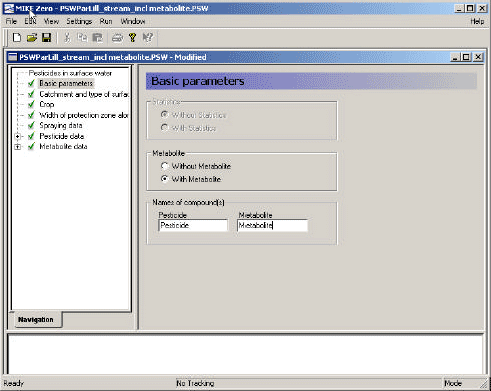
Figure 3.3 Menu page: Basic Parameters.
Figur 3.3 Menu-side: Basale parametre.
Initially, it was intended that the user interface should allow automatic selection of Monte Carlo parameters. This function has been not been implemented and is therefore not active. As the stream runs take about 24 hours, the time required to run a distribution of parameters is considerable.
3.3.2 Catchment and type of surface water
In the second menu (Figure 3.4), the scenario is selected. This includes
- the location (Lillebæk/Odder bæk), which is actually an expression of the type of landscape represented, Lillebæk being moraine and Odder Bæk representing more sandy conditions,
- the type of water body (stream/pond) and
- whether the pond is aerobic (macrophyte-dominated) or anaerobic (phytoplankton-dominated).
With the second menu completed, all the required files of Table 3.1, and the four file types of Table 3.3 are defined.
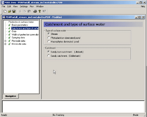
Figure 3.4 Menu-page: Catchment and type of surface water.
Figur 3.4 Menu-side: Opland og type af overfladevand.
3.3.3 Crop
The third menu (Figure 3.5) allows the user to choose the crop to be sprayed, and to set a transpiration factor for the active substance. The transpiration factor is a factor that defines the plant uptake of pesticide. The value may vary between 0 and 1, and is multiplied onto the concentration of the water taken up. In test runs it was noted that for spring applications, particularly in the moraine catchment, the model is very sensitive to this value, as a considerable part of the pesticide is taken up by plants, even with a transpiration factor of 0.4.
For spruce trees, the choice also concerns the age of the culture and whether it is sprayed horizontally. The reasoning for these choices are described in Section 2.1 and 2.2, but in short, the coverage percentages and the function used to calculate wind drift differ depending on plant age and spraying method.
With the selection of crop, the selection of water movement file is finalised. The choice also determines the type of wind drift formula to use.
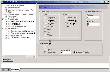
Figure 3.5 Menu-page: Choice of crop. Spring wheat and spring barley uses the same pre-calculated water file.
Figur 3.5 Menu-side: Valg af afgrøde. Vårhvede og vårbyg bruger de samme for-beregnede vandfiler.
3.3.4 Width of protection zone
The next menu allows the user to select the width of the buffer zone. The choice influence the calculation of wind drift (Section 2.1), the calculation of dry deposition (Section 2.3.2) and the choice of file describing the size of agricultural land. As the grid size of the model is 50 m, the area to be sprayed cannot be successively reduced. If the buffer zone is greater than 35 m, the row of grids closest to the stream on both sides is removed from the sprayed area. The choice thus influence the selection of file specifying the sprayed area, the agrl_0 or agrl_35-file mentioned in Table 3.3.
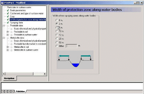
Figure 3.6 Menu-page: Width of protection zone.
Figur 3.6 Menu-side: Bredde af bufferzonen.
3.3.5 Spraying data
The specification of the spraying data requires a dose and a date. To take into account the effect of date of spraying, the model should be run several times, with different possible spraying days selected in the relevant period of spraying. If, for example, the spraying period is 1st to 20th of May, the model could be run 4 times, e.g. on 1st, 6th, 11th, and 16th of May 2. This pr°Cedure is also used for the Danish grounDwater scenarios. The user can choose to allow or not allow spraying when rain occurs. If the user do not allow this, the spraying date is moved forward by eight hours until a period with no rain is encountered. As four different years are simulated, it is found somewhat artificial to find dates that in all years will fulfill particular criteria – this will allow very few spraying dates during the year.
More sprayings are specified by clicking on the "extra line" bottom (top left), and a new dose and the number of days between the first and the second spraying can be specified.
The dose is input to the wind drift calculation, the calculation of dry deposition and the further calculation in the soil. The correction of the dose to the soil is already described in Section 2.2.
When the spray drift and dry deposition has been calculated, time series files are generated for each stretch of the river or for the pond, containing the deposition of active substance on the water body over time.
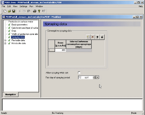
Figure 3.7 Menu-page: Spraying data.
Figur 3.7 Menu-side: Sprøjtedata.
3.3.6 Basic chemical and physical properties of the active substance (and metabolite)
This menu (Figire 3.8) exists both for the active substance and metabolite 3.
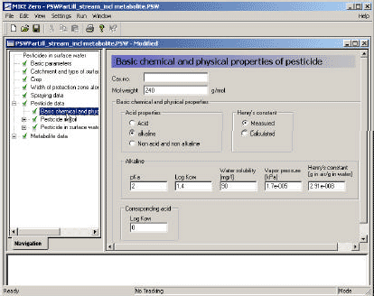
Figure 3.8 Basic chemical and physical properties.
Figur 3.8 Basale kemiske og fysiske egenskaber.
The Cas number is specified as a text string.
The basic chemical properties of an active substance (or a metabolite) that have to be specified are:
- the molar weight,
- the pKa, the Kow of the neutral compound,
- the water solubility of the neutral compound (mg/l), and
- the vapour pressure (kPa).
Henry's constant can be should preferably be specified, but if not, it is calculated as
Henry's constant =
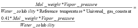
(Eq. 65)
where mol weight (g/mol), the vapour pressure (kPa) and the water solubility stem from the interface,
Universal_gas_constant = 0.0821 l*atm/mol*k
Reference temperature = 293 K, and
the transformation factor is 9.85E-06 Pa/atm
The assumed reference conditions are 20ºC and 1 atm. If the active substance is an acid or a base, Kow is re-calculated to fit the pH-value of the scenarios. Otherwise the Kow-value is used directly in the calculations. The transformations are done in the following manner:
if the compound is neutral
Kow=Kow_1
if the compound is an acid
(Eq. 66)
if the compound is a base
(Eq. 67)
The dry deposition programme utilises the vapor pressure and Henry's constant. The pKa-value is used to modify the dose available for evaporation (InputDryDepositionCalculations.txt). For all scenarios pH was set to 7.6.
The solubility of the compound is used in MIKE SHE as a maximum concentration allowed for distributed pesticide (.tsf-file). This mainly influences the colloid transport processes.
All of these parameters are used for the MIKE 11-calculations (*.PE11-file)
3.3.7 Sorption of active substance in soil
With respect to sorption in the soil, the user may choose between a linear and a Freundlich isotherm.
The default value for the exponent of a Freundlich isotherm is 0.9. The Freundlich isotherm is defined as x = Kfcref(c/cref)1/n, where x is the content of active substance sorbed (mg/kg), and c is the concentration in the liquid phase (mg/l). cref is the reference concentration, which is usually 1 mg/l. K must be given in dm3/kg (or l/kg).
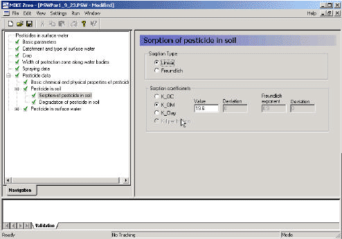
Figure 3.9 Menu-page: Sorption of active substance in soil.
Figur 3.9 Menuside: Sorption af pesticid i jord.
It is important to note that if the Freundlich isotherm is used, the value of Kf is very sensitive to the units. In MIKE SHE, the internal calculations are in g/l and a transformation is therefore carried out as part of the pre-processing programme for sorption values used for Freundlich sorption:
![]()
(Eq. 68)
where
N = 1/n
K = Kf in mg/l
The sorption coefficient can be defined as a function of organic matter (KOM), as a function of organic carbon (KOC), as a function of clay (Kclay) or as a Kd-value of the soil. As % OC = % OM/1.724, KOC = KOM * 1.724. If KOC, KOM or Kclay is given, the sorption of each horizon in each soil profile is calculated as a function of the organic matter content or clay content of the respective horizon.
The equivalent Kd-value is the Kx * the fraction of the 'x' constituent of the soil. Maps of each of these constituents have been prepared (Table 3.3). The result of the pre-processing is therefore a series of maps (T2-files) of Kd-values that are referred to in the xtsf-file.
If nothing else is known, the user can estimate sorption from KOW in the following manner: log10(KOC) = 1.029*log10(KOW) – 0.18.
The value can also be used as input to the calculation of Kd for the MIKE 11 model of rivers and ponds, (see Section 3.3.9). To avoid an extrapolation to active substances concentrations far below the concentrations at which the empirical Freundlich equation was derived, linear sorption is always assumed for the streams and ponds.
A similar page should be filled out for the metabolite, if a metabolite is included in the calculation.
3.3.8 Degradation of active substance in soil
The menu allows specification of a degradation half life in days at 20 °C and at a moisture content equal to of either pF1 or pF2. The user also specifies a relative change in degradation rate with depth. The default values given are 1 from 0-30 cm's depth, 0.5 from 30-60 cm depth and 0.3 from 60 cm to 1 m. Note, that these values are corrections of the rate, and the DT50-value is thus inversely related to this factor.
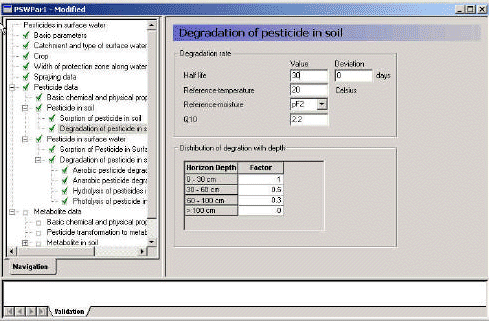
Figure 3.10 Menu-page: Degradation of active substance in soil.
Figur 3.10 Menu-side: Nedbrydning af pesticid i jord.
It is possible to specify a Q10 value, this is the relative change in reaction velocity by a change in temperature of 10 degrees. The default value is 2.2 (FOCUS, 1996).
As the internal reference moisture content in MIKE SHE for degradation is the moisture content at saturation, the DT50 at pF1 or pF2 is re-calculated to DT50 at saturation. The formula used is:
![]()
(Eq. 69)
As this correction factor depends on the soil type, the correction factors are prepared as maps for different soil depths (see Table 3.3). The DT50 values are then corrected with the changes in degradation rate with depth (the inverse value is used on the DT50 as DT50 and degradation rate is inversely related). The result is a series of T2-maps of the DT50-values, referred to in the xtsf-input file.
The defined layers in Lillebæk and Odder Bæk follows horizons and discretisation. These layers are slightly different from the standard depths given for depth correction factors. Table 3.4 shows how the correction factors are used on the different layers in the two catchments.
Table 3.4 Utilisation of (default) depth correction factors on the layers defined for the Lillebæk and Odder Bæk-scenario.
Tabel 3.4 Anvendelse af (standard) dybdekorrektionsfaktorer for lagene defineret i Lillebæk-og Odder Bæk scenariet.
| Lillebæk | Odder Bæk | ||
| Depth, cm | Depth correction factor | Depth, cm | Depth correction factor |
| 0-30 | 1 | 0-25 | 1 |
| 30-40 | 0.5 | 25-35 | (1+0.5)/2 |
| 40-45 | 0.5 | 35-60 | 0.5 |
| 45-50 | 0.5 | 60-80 | 0.3 |
| 50-70 | (0.5+0.3)/2 | 80-100 | 0.3 |
| 70-80 | 0.3 | 100-150 | 0 |
| 80-100 | 0.3 | > 150 | 0 |
| 100-105 | 0* | ||
| 105-120 | 0 | ||
| 120-170 | 0 | ||
| >170 | 0 |
- As DT50-values are specified, and the rate is specified as the inverse value, a zero equals an infinitely large DT50-value. However, the model interprets a "0" as "no degradation".
In the model, the reference degradation rate is calculated as μ ref = ln2/(half life). The degradation rate is then modified according to temperature and moisture content according to the following formulas:
μ = μ ref* Fw*Ft, where
Ft = e α(T-Tref)
α= (lnQ10)/10 (for Q10 = 2.2,α = 0.079 K-1)
Fw = (θ /θ b)0.7
A similar page should be filled out for the metabolite, if a metabolite is included in the calculation.
The final maps produced are stored under \MAPS and referred to in the .xtsf-file.
3.3.9 Sorption of active substance in surface water
The menu page "Sorption of active substance in surface water" allows the user to choose between the use of the KOC, KOM, Kclay from soil or whether to calculate a value from Kow. If the user choose to calculate the Kd value from the sorption data given for the soil (Section 3.3.7) the following pr°Cedures are applied:
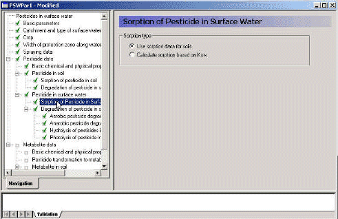
Figure 3.11 Menu-page: Sorption of active substance in surface water.
Figur 3.11 Menu-side: Sorption af pesticid i overfladevand.
If the input is KOC
Kd_Water = Kd_sediment = (KOC*LOI_Scen*1.724/ 1*106), where
LOI_Scen =Loss of ignition, weight % for the specific scenario.
If the input is Kom
Kd_Water = Kd_sediment = (Kom*LOI_Scen)/1*106, where
LOI_SCEN =Loss of ignition, weight% for the specific scenario.
If the input is Kclay
Kd_Water = Kd_sediment = (Kclay*(Clay_content))/1*106
where
Clay_content = Clay content for the specific scenario
The formulas used for calculation of Kd as a function of Kow are:
![]()
(Eq. 70)
where
Kow stems from the interface
LOI_Scen =Loss of ignition, weight % for the specific scenario
The loss of ignition values appear from Appendix F.
In addition the desorption rate is calculated from the following equation:
Desorption_Water = desorption_sediment = Sorption_rate/(Kd_Water*CP),
(Eq. 71)
where
Sorption_rate: 2.9
CP 83333 gm-3
To avoid an extrapolation to active substances concentrations far below the concentrations at which the empirical Freundlich equation was derived the Freundlich isoterm is always set to 1 when the sorption in the river was determined. Hence for the rivers linear sorption was assumed.
A similar page should be filled out for the metabolite 4, if a metabolite is included in the calculation.
The information is transferred to the .PE11-file.
3.3.10 Aerobic degradation of active substance in surface water
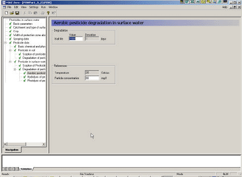
Figure 3.12 Menu-page: Aerobic degradation of active substance in surface water.
Figur 3.12 Menu-side: Aerobisk nedbrydning af pesticid i overfladevand.
A major aim of the sorption and biodegradation experiments of (Helweg et al 2003) was to develop an approach for estimation of the biodegradation of active substances in the sediment and in the water column. Ideally the approach should consider both the reduced bio-availability of the active substances in the sediment caused by sorption to particles and the relative differences in the bacterial activity in the sediment and the water column.
The approach is based on the following consideration:
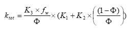
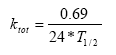
From the user interface is a total biodegradation rate derived by the following equation:
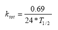
(Eq. 72)
where T1/2 (days) is specified in the interface,
0.69 = ln(2),
24 is hours/day.
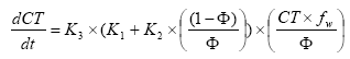
Or the total degradation of the active substance from the user interface might be described by the differential equation:
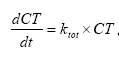
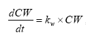
(Eq. 73)
where
CT denotes the total degradation of the active substance.
It is assumed that only dissolved active substances is degraded and that the degradation is attributable both to free living (pelagic) and to bacteria associated with particles. The activity of free living bacteria is assumed to be the same in the pore water and in the water column, whereas the activity of bacteria associated with particles is assumed to be proportional to the concentration of particles. Finally is it assumed that the degradation of active substances is proportional to the bacterial activity.
The degradation of the dissolved active substance might then be described by the following differential equation:
(Eq. 74)
where
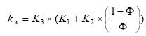
(Eq. 75)
where
K1 denotes the relative activity of free living bacteria,
K2 denotes the relative activity of bacteria associated with particles,
K3 denotes a active substance specific degradation rate per bacterial activity,
Φ denotes the porosity of the suspension applied in the experiment.
Furthermore is it assumed that the bio-degradation rate is much lower than the sorption rate, which is supported by the sorption experiments of (Helweg et al 2003). If such the distribution of active substances between water and particles might be described by the following equation:
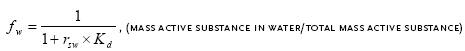 , (mass active substance in water/total mass active substance)
(Eq. 76)
where
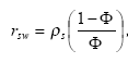
(Eq. 77)
where
ρs denotes mass density of the sediment particles
The relationship between the total concentration of active substance sorbed to particles and the concentration of dissolved active substance can then be written as:
![]()
(Eq. 78)
and (74), (75), (77) and (78) is combined to:
(Eq. 79)
and
(Eq. 80)
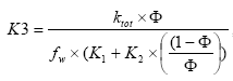
K2 and K1 are constants determined from the experiments of (Helweg et al 2003). The menu allows specification of a total degradation time for an experiment conducted at a given particle concentration.
The model requires specification of the bio-degradation in porewater, in the dissolved phase and on macrophytes. These values are derived from the total degradation as follows:
(Eq. 81)
where
T1/2 (days) is specified in the interface
0.69 = ln(2)
24 is hours/day.
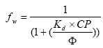
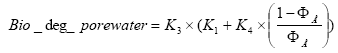
![]()
(Eq. 82)
where
Φ is the porosity of the experiment of the user interface,
CP = the particle concentration of the experiment of the user interface (mg/l).
(Eq. 83)
where
fw = mass fraction of active substance in water and particles for the experiment of the user interface,
CP = the particle concentration of the experiment of the user interface (mg/l),
Kd values for the respective scenario determined from Section 3.3.9.
(Eq. 84)
where
K3 a active substance specific degradation constant,
CP the particle concentration of the experiment of the user interface (mg/l),
K1 a constant derived from the biodegradation experiments of (Helweg et al 2003),
K2 a constant derived from the biodegradation experiments of sub-project 5 (Helweg et al 2003).
Thereafter the degradation rates is calculated in the following way:
(Eq. 85)
![]()
(Eq. 86)
where
K4 Is a constant estimated on the basis of the calibration exircise for the pond models (Styczen et al 2004)
Values for K1, K2 and K4 appear from Appendix G.
The results are transferred to the PE11-file. A similar page should be filled out for the metabolite, if a metabolite is included in the calculation.
3.3.11 Anaerobic degradation of active substance in surface water
Anaerobic biodegradation is applied for the degradation of dissolved active substance in the pore water of the sediment in the phytoplankton dominated pond. The influence of particle concentration, or porosity, is taken in to account as described in Section 3.3.10.
The menu-page is identical to aerobic degradation (Figure 3.12) A similar page should be filled out for the metabolite, if a metabolite is included in the calculation.
3.3.12 Hydrolysis of active substance in surface water
The model interface allows specification of a half life for acid, basic and neutral hydrolysis. When hydrolysis experiments conducted at different pH is available the different values is readily calculated using for instance an excel spreadsheet, solving three of the following equations with three unknowns:
Measured Rate = Kacid[H+] + Kneutral + Kbasic[OH-]
An example of such a spreadsheet will be delivered together with the final model.
These are re-calculated to rates as
![]()
(Eq. 87)
![]()
(Eq. 88)
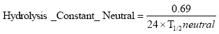
(Eq. 89)
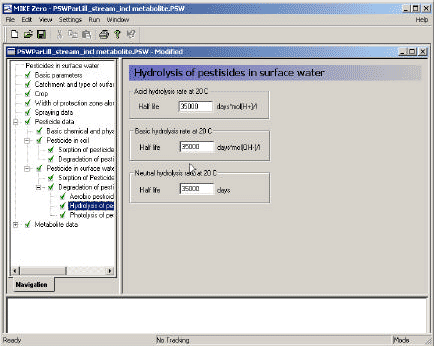
Figure 3.13 Menu-page: Hydrolysis of active substance in surface water
Figur 3.13 Menu-side: Hydrolyse af pesticid i overfladevand
A similar page should be filled out for the metabolite, if a metabolite is included in the calculation.
3.3.13 Photolysis of active substance in surface water
For description of photolysis the user is required to specify the absorption spectrum of the compound, and the quantum yield. The quantum yield specifies how many mol of active substance that is degraded by one mol of photons absorbed. In addition the spectral composition of the light in the summer season and a time series of the global radiation at the surface is used by the model, as mentioned in Table 3.2. The global radiation data was measured data for Hornum(st. nr. 20501), which was considered to be representative for normal Danish conditions. The global radiation data is given for every day in the periods used for the scenarios. The composition of the solar insulation was calculated from data given by OECD (1995). On the basis of these information the photolytic decay is calculated as described in Section 2.5.7.
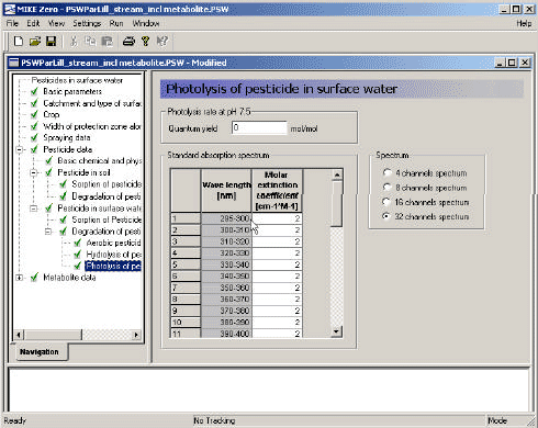
Figure 3.14 Menu-page: Photolysis of active substance in surface water
Figur 3.14 Menu-side: Fotolyse af pesticid i overfladevand
A similar page should be filled out for the metabolite 5, if a metabolite is included in the calculation.
3.3.14 Pesticide transformations to metabolite
The transformation of active substance to metabolite is not a one to one process. First of all, the metabolite is smaller than the active substance, and secondly, only a fraction of the active substance (fprocess)turns into this particular metabolite. The difference in molar weight is taken care of by the pre-processing programme, as the molar weights are dealt with elsewhere. The factor that has to be specified is the fraction of active substances (in terms of mol) that turns into this particular metabolite.
The fraction is specified for different processes, as it is not certain that all processes have the same stochiometry.
fweight, process = fprocess * mol weightmetabolite/mol weightpesticide
The fraction is transferred to the xtsf-file and the pe11-file and is used to define the production of metabolite:
1 g of degraded active substance => fweight,process g of metabolite.
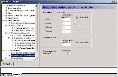
Figure 3.15 Menu-page: active substance transformation to metabolite
Figur 3.15 Menu-side: Pesticid'ets omdannelse til metabolit
Footnotes
[1] The first 2 hours after spraying, results are stored every 10 minutes. For the next 30 days, data are stored every hour. During the rest of the simulation, data are stored every 3rd day.
[2] Comment from reviewer: Given the event-driven nature of the pesticide exposure, the possibility to select different application dates will result in a wide range of calculated exposure concentrations for a specific crop. In my view it would be wise to limit the possibilities of selecting an application date or a very limited number of possible application dates.
[3] The programme presently uses the value given for Henry's constant and solubility for the pesticide also for the metabolite.
[4] The programme presently uses the value given for sorption for the pesticide also for the metabolite.
[5] The programme presently uses the value given for quantum yield and adsorption spectrum for the pesticide also for the metabolite.
Version 1.0 Maj 2004, © Danish Environmental Protection Agency