|
Geographical, technological and temporal delimitations in LCA 2 Market-based system delimitation
2.1 Building product system modelsTo build a model of a product system, it is natural to start with the process in which the reference flow occurs (see the guideline “The product, functional unit and reference flows in LCA” for more information on how to determine the reference flow). Each item in the reference flow is then linked to the next process both backwards and forwards in the life cycle. Backwards, the flow typically consists of intermediate products, components, ancillary inputs, and raw materials. Forwards, the flow may also consist of final products, products for reuse or recycling, and waste to treatment. To make it simple, we call all these flows “intermediate product flows”. Flows to the environment (environmental exchanges) are typically not included in the first description of a product system. The purpose of the procedure presented in section 2.2 is to determine the process(es) that a specific intermediate product flow should be linked to, and which therefore should be included in the studied product system. It is for these processes that data on environmental exchanges are later to be collected. The overall uncertainty of a life cycle assessment will often be determined by what processes are included and excluded from the analysed product systems. The procedure applies to each intermediate product flow between processes in the life cycle, but it may not be necessary to apply the entire procedure in detail for all intermediate products. The procedure is primarily intended as a guideline for those instances where it is not immediately obvious which processes are to be linked. This may be the case when there are many possible suppliers with very different production conditions or when one or more of the possible suppliers cannot immediately change production volume in response to a change in demand. In a first iteration, the procedure should only be applied for such cases of constraints in production volumes (see section 2.2.4), or where there is an order-of-magnitude difference in expected environmental exchanges between different possible processes (see also section 2.4 for a discussion of uncertainty of the procedure). It should be noted that the suppliers that are identified by the procedure, and for which data on environmental exchanges are later to be collected, are not necessarily a part of the current supply chain. The market information required for the procedure is typically available from marketing personnel dealing with each specific market. The collection of the necessary information has been found to be much less demanding than the collection of data on the environmental exchanges of each process. When the necessary market information cannot be made available, the default assumptions and default data from section 2.3 can be applied. 2.2 ProcedureSince the purpose of a life cycle assessment is to assess the possible environmental impacts of a potential product substitution, it is the processes affected by this product substitution that should be included in the studied product systems. A product substitution (e.g. the choice of one chair design instead of another) will result in a change in demand for the intermediate products that enter into the process in which the substitution occurs (e.g. the steel and plastic components that are used by the chair manufacturer), and likewise in the demand for the further intermediate products backwards in the life cycle (e.g. the plastic raw materials). The procedure presented here identifies the processes that are expected to be affected by such a change in demand for a specific intermediate product. A product substitution will also result in a change in supply of the intermediate products leaving the process in which the substitution occurs, and in supply of the further intermediate products forwards in the life cycle (e.g. the distribution, retail sale, use and disposal of the chair). To make the description less abstract, the explanatory text in this section only covers the situation where an intermediate product is followed backwards in the life cycle (identifying the effects of changes in demand). However, the 5 steps of the procedure, the decision tree in figure 2.1, as well as the general concepts in the explanatory text, are also applicable when following an intermediate product flow forwards in the life cycle (identifying the effects of changes in supply). By the procedure presented here, one or more suppliers will be identified as being affected by a change in demand. The identified suppliers will typically use a specific technology and/or be located within a specific geographical region (since differences in market conditions and competitiveness typically depend on geographical and technological differences). The number of suppliers and the degree of detail of describing their technologies, depends on:
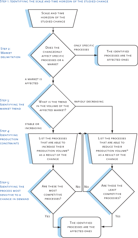
Figure 2.1 Decision tree outlining the 5-step procedure for identifying the processes affected by a change in demand for a specific intermediate product. Please se the text for detailed explanations
*) For long term changes, the volume relates to production capacity, while for short term changes it relates to output within the existing capacity, see also the text in section 2.2.1 and 2.2.1 Step 1: Identifying the scale and time horizon of the studied changeBefore it can be determined what suppliers/technologies that may be affected by a change in demand for an intermediate product, it is necessary to know the scale and time horizon of the change. Scale of change Large changes are typically seen when introducing new technology or new regulation on a significant market, e.g. if all cars were to be made from polymers and carbon fibres in stead of steel, which among other consequences would have the market for steel turning from increasing to decreasing. However, many small changes may accumulate to bring about a large change. Therefore, even in studies of small changes it may sometimes be relevant to apply an additional scenario with the possible larger changes that could be the result of accumulated small changes. For example, even in a life cycle assessment considering such a shift to polymers and carbon fibres for a single producer of cars, it may be relevant to investigate the possible consequences of other car producers following suit. Time horizon
In general, changes cannot be isolated to the short-term, since capital investment (i.e. long term changes) is typically a continuous process affected by the current and expected trends in the market volume, resulting from the accumulation of a large amount of individual short-term purchase decisions. This is obvious in markets with a short capital cycle (fast turnover of capital equipment, as e.g. in the electronics and polymer industries) and in free market situations (where market signals play a major role when planning capacity adjustments), but it is also true for markets with a long capital cycle (as e.g. in the building and paper industries). Thus, the isolated effects of short-term changes (i.e. effects within the existing production capacity) are only of interest in markets where no capital investment is planned (e.g. industries in decline), or where the market situation has little influence on capacity adjustments (i.e. monopolised or highly regulated markets, which may also be characterised by surplus capacity). Office chair example
Office chair example: This and the following steps in the procedure will be illustrated with examples taken from an LCA of an office chair. The LCA concerns the design for improved reuse of a
specific brand of office chairs.Thus, it is a case of a small change (since it concerns only one specific producer, not the entire market) with a long time horizon (since the new design can be
expected to affect future capital investment in the different processes in the life cycle). An example of a change with a short time horizon could be an isolated decision to remove heavy metals from the polymers and surface coatings of the chair, which – all other things equal –
would not involve capital investment in the metal industry, since heavy metals are already being phased out. 2.2.2 Step 2: Market delimitationGiven the scale and time horizon of the studied change, the next step in the procedure is to determine the possible suppliers of the intermediate product. Market ties
Many examples can be found of the latter situation, especially:
If a specific supplier (or group of suppliers) is identified as the one affected, it may be useful to justify that the production volume of this process is actually able to change. For this purpose, step 4 in the procedure (section 2.2.4) may be applied. The procedure can only be terminated here if the production volume of the specific suppliers is actually expected to change as a result of the studied product substitution, i.e. as a result of a change in demand for the intermediate product. If the change in demand is transferred on to other suppliers of the intermediate product, the production volume of the specific supplier will not change. This may be the case in spite of close relations between supplier and customer, even in spite of ownership relations or sole-supplier-status, i.e. it is not the closeness of the relation, which is important, but whether the overall production volume of the supplier is actually expected to be affected. An example of this is in-house electricity production. If the in-house production fluctuates with in-house demand and thereby does not affect the production volume of the general electricity market, then the in-house production can be regarded as the affected electricity source for the in-house demand. However, if the in-house production takes place on normal market conditions, and the in-house production does not fluctuate with in-house demand (even when the company is closed), then the electricity supply for the in-house demand must be regarded as coming from the general electricity market, and not from the specific in-house production. This also means that a life cycle assessment will only give credit for - and incentive to - a shift to specific products or suppliers with more environmentally friendly technologies, e.g. “green electricity”, when this shift is actually expected to lead to an increase in the capacity of the “green” technology. If the shift only pretends to be an improvement, and no change is expected in the composition of the overall output, no credit is given. However, the effects of a shift may be delayed, so that the expected increase in the “green” technology will only appear after some time. An example of this may be the initial immature market for ecological foods, where an increase in demand may not lead to an increase in production, because of the transaction costs of the initial small quantities or because of the time it takes to implement the new technology on the farms. In such instances, a demand for “green” products should still be credited for its long-term influence on the production capacity of the “green” technology. Also, the effects of a shift may be indirect, via the political signal that it sends. For example, a constraint on a specific “green” product may be overcome, e.g. by political intervention or because a private company takes up the challenge, as a result of a consistent unsatisfied demand for this product. Likewise, a consumer boycott of a particular product may be followed up by political action or “voluntary” changes in company behaviour that limits the production beyond the effects of the boycott itself. Since such indirect effects may be controversial and difficult to predict, it may be preferable to include them in separate scenarios. Market identification
The identification of the obligatory product properties and the geographical and temporal market boundaries is parallel to the first two steps described in the guideline “The product, functional unit, and reference flows in LCA”. While the description in that guideline may be useful also for intermediate products, it should be noted that the procedure does not need to be elaborated in detail for every intermediate product. Office chair example
Office chair example: For most of the materials in the office chair (mainly steel and plastic materials), several suppliers are possible. These materials are traded on a competitive market
without specific ties between suppliers and customers. Therefore, a change in demand from the office chair manufacturer cannot be expected to only affect the current suppliers, but will rather
affect the entire market for these materials. This market can be identified as being European, since for steel and plastic materials, Europe constitutes a fairly closed market, as can be seen e.g.
from Eurostat production and trade statistics databases and publications (EUROPROMS; Panorama of European business; Intra- and extra-EU trade, and Iron and steel yearly statistics). 2.2.3 Step 3: Identifying the market trendWithin the identified market, not all suppliers will be equally affected by a change in demand. For short-term changes (see also section 2.2.1), the affected suppliers will typically be the least competitive (often using older technology), since it is mostly these suppliers that have capacity available. For long-term changes, the affected suppliers depend on the overall market trend. In a market that decreases (at a higher pace than what can be covered by the decrease from regular, planned phasing out of capital equipment) the affected suppliers will typically be the least competitive. If the market is generally increasing (or decreasing at a rate less than the average replacement rate for the capital equipment), new capacity must be installed, typically involving a modern, competitive technology. Therefore, it is important to identify the market trend (“Is the market increasing or decreasing?”) especially for long-term changes involving capacity adjustments. It follows from the above distinction, that if the general market volume is decreasing at about the average replacement rate for the production equipment, the effect of a change may shift back and forth between suppliers with very different technologies, which makes it necessary to make two separate scenarios. This may be relevant for a fairly large interval of trends in market volume, since the replacement rate for production equipment is a relatively flexible parameter (planned decommissioning may be postponed for some time, e.g. by increasing maintenance). Note that it is the overall market trend, which is of interest, and not the direction of the specific demand studied. This is because - as long as the overall trend in the market is not affected – it is the same suppliers that will be affected by an increase in demand and a decrease in demand. The trends in market volumes should preferably be determined using the same kind of information as that available to those deciding on capacity adjustments in the affected industry. This information is typically a combination of statistical data showing the past and current development of the market and different forecasts and scenarios. If no information is available, it is safest to assume that the market is increasing, since this is the most typical situation. Office chair example
Office chair example: For most of the materials in the office chair the market trend is increasing.Trade statistics and forecasts are available from industry associations and consultants, for
steel e.g. the International Iron and Steel Institute (http://www.worldsteel.org/) and World Steel Dynamics (http://www.worldsteeldynamics.com/). Despite an increasing global trend, the
European production of steel is stagnating, however not below the replacement rate of the production equipment.This implies that the affected suppliers are to be found among the most
competitive steel makers in Europe, since it is here that new capacity is being installed. The result of this step is that we can concentrate our search for the affected suppliers to one end of the market, either among the most competitive (for long-term changes in an increasing market) or among the least competitive suppliers (for long term changes in a rapidly decreasing market and for short-term changes). 2.2.4 Step 4: Identifying production constraintsThe possible suppliers (among the most or least competitive, depending on the conclusion of the previous step) may be subject to constraints that render them unable to react to a change in demand with a change in production volume. Since their production volume (and environmental impacts) cannot be affected by the studied change in demand, such constrained suppliers should not be included in the product system. A supplier or an entire technology can be constrained in its ability to change its production volume in response to a change in demand, for one or more of the following reasons:
In some cases, an entire market may be constrained, so that none of the suppliers will change their production volume in response to a change in demand. The change in demand will instead mean a change in the supply of the intermediate product to that application area (or customer) of the product, which is most sensitive to a change in supply. Here, the change in supply will imply an equivalent change in consumption. Production constraints may change:
Thus, it is important to note the conditions for which the constraints are valid. Especially, when studying long-term changes (the typical situation for life cycle assessments, see section 2.2.1), it should be avoided that a process is excluded from further considerations because of constraints that only apply in the short term (in day-to-day operations, many constraints apply, e.g. in raw material availability and production capacity, that are irrelevant when considering long-term changes). In case of missing information on production constraints, it must be tentatively assumed that there are none. Unjustified exclusion of processes is thereby avoided. If a constrained process is thereby included, this will normally be discovered in the next step in the procedure. Office chair example
Office chair example: A change in demand for steel in the office chair cannot affect plants that use the electric arc furnace (EAF) technology, since this technology is constrained by the
availability of its main raw material (steel scrap).This leaves only the basic oxygen furnace (BOF) technology to be affected by a change in demand from the office chair manufacturer. Note
that we assume a small change with a long time horizon (see step 1), so that we expect the same reaction to an increase in demand as to a decrease in demand, and we look at changes in
production capacity. 2.2.5 Step 5: Identifying the suppliers/technologies most sensitive to a change in demandAmong the unconstrained suppliers/technologies, some will be more sensitive to a change in demand than others. For long-term changes in an increasing market, the most sensitive supplier/technology is identical to the most competitive, while in a rapidly decreasing market and for short-term changes, the most sensitive supplier/technology is the least competitive (see section 2.2.3). Competitiveness is typically determined by the production costs per unit. For capacity adjustments it is the expected production costs over long-term that matters. The distinction between constraints (section 2.2.4) and costs is not completely sharp, since some constraints may be translated into additional costs and some costs may be regarded as prohibitive and therefore in practice function as constraints. However, if not taken too strictly, the distinction is useful for practical decision making. Also the definition of costs itself is not sharp, since concerns for flexibility (as a concern for future costs), environmental costs and other externalities – whether monetarised or not - may enter the decision-making process. When predicting the actual decisions with regard to changes in capacity or capacity utilisation, it is therefore necessary to include all those constraints and nonmonetarised costs which are relevant to the decision makers, but on the other hand not such which are not going to influence the actual decisions. The kind of costs included may also vary depending on the interests of the decision makers, e.g. private investors may place less emphasis on environmental externalities than a public investor. Thus, the most sensitive suppliers/technologies are determined from the production costs, while taking into account constraints and non-monetarised costs as perceived by those who decide about the change in capacity (longterm) or capacity utilisation (short-term). The important point is to model as closely as possible the actual decision making context. Data on production costs for individual plants, countries, or technologies are obtained from the industry in question, from industry consultants, or from research organisations, for steel e.g. World Steel Dynamics. If data cannot be obtained, it may be assumed that modern technology is the most competitive and the oldest applied technology is the least competitive. With respect to geographical location, it can be assumed that competitiveness is determined by the cost structure of the most important production factor (labour costs for labour intensive products, else energy and raw material costs). When comparing labour costs, local differences in productivity and labour skills should be taken into account. Office chair example
Office chair example:The source of the crude oil used for producing the plastic parts in the office chair will come from the most competitive oil sources (since the oil market is increasing).
According to the International Energy Agency (http://www.iea.org/),World Energy Outlook 1994, the most competitive sources (those with the lowest extraction costs) are the sources in the
Middle East and Venezuela, which are expected to increase their share in the global supply from 30% in 1991 to 45-57% in year 2010. 2.3 Default assumptionsFor the initial phases of a life cycle study, and for parts of the life cycle that are less important, the procedure described in section 2.2 may be too elaborate and too demanding. Also, there may be situations where it is not possible to obtain the necessary market information. In these situations, the defaults in table 2.1 may be applied. The detailed arguments for these defaults are given in LCA Report No. 1: Market information in LCA. Table 2.2 lists some typical processes, which may be assumed to be the ones affected by a change in demand for the listed products under the stated conditions. When used in a specific study, please check whether the stated conditions apply. The conditions stated in table 2.2 are the expected conditions on the European market in the years 2000-2010, provided that the studied changes are small. Unless otherwise stated, the defaults in table 2.1 apply. The main differences in assumptions between the products relate to differences in market trend (increasing to stable versus rapidly decreasing) and geographical market boundaries (local, continental or global). For documentation and sources of these assumptions, please see the background report “Market information in LCA”. It can be seen from table 2.2 that the specific affected suppliers/technologies are often very different from the corresponding average supplying the market. Thus, only in exceptional cases can average data be used as proxy data, when market-based data are not available. This may e.g. be the case when the market in question is supplied exclusively by one main, slowly developing technology. In most other situations, it is preferable to make one or more estimates of the affected process, based on the available data. Table 2.1. Default assumptions on market conditions
* In that transport costs have been attributed large importance here. However, also other factors may be of significance, such as possible toll barriers, trade patterns, and geographical differences in overall production volume. If you have data for a market average, the market range may be estimated by coefficients of variance of:
When the range is known or has been estimated, the affected process can then be assumed to be at one of the ends of this range, depending on realistic assumptions with respect to the items listed in table 2.1. It is thereby assumed that all the above exchanges co-vary, so that large energy consumption is linked to large raw material consumptions and large exchanges to the environment. When relevant, several alternative scenarios should be included to reflect the limits of knowledge. Table 2.2 Default list of processes affected by a change in demand for selected products, under the expected conditions for the European market in the years 2000-2010 and when the studied changes are small
2.4 Uncertainties in identifying the correct processes to includeThe procedures for identifying the correct processes to include in the studied product systems, as described in section 2.2, rely on market data, in which the following uncertainties are of importance:
These uncertainties will often be dominating the overall uncertainty of a life cycle assessment, since they may affect which processes are included and excluded from the analysed product systems. The importance increases in proportion to the possible variation in the technologies and processes that may be substituted, i.e.:
This means that the higher the variation in possible outcomes, the higher is the demand on the quality of the market data. A reduction of the uncertainty can only be obtained through a better understanding of the different intermediate products in the life cycle and the markets on which they are traded. Thereby, the individual processes to be included in the product system can be determined with more precision. Use of quality assurance and critical review as part of the life cycle assessment can contribute to the reduction of uncertainties. The above considerations are also valid for the standard assumptions in traditional system delimitation (see section 1.3), but since this does not include market information it will be difficult to estimate the real uncertainties as a result of the system delimitation. The uncertainty on a traditionally delimited system will therefore typically be calculated from the uncertainties on the average data for the included processes. Since this uncertainty is an expression of a real variation, it cannot be reduced through additional data collection. When relevant, several alternative scenarios should be included to reflect the limits of knowledge. The mentioned major sources of uncertainty also apply to the handling of multi-functional systems, following the procedure described in chapter 3. The issue of uncertainty is dealt with in more detail in the technical report “Reducing uncertainty in LCI.”
|