| Front page | | Contents | | Previous | | Next |

Geographical, technological and temporal delimitations in LCA

4 Forecasting procedures

• 4.1 Introduction
• 4.2 Determining the parts of the product systems for which forecasting is relevant
• 4.3 Determining the necessary detail of forecasting
• 4.4 Choosing the relevant forecasting method
• 4.5 Forecasting by extrapolation

4.1 Introduction

The previous chapters included considerations on the time horizon of the studied change, and it was made clear that the processes to include in the studied product systems may change over time, depending on the future market situation. However, no recommendations were given for the actual forecasting procedures to be applied. This is the topic of this chapter.

4.2 Determining the parts of the product systems for which forecasting is relevant

It may not be equally important to forecast all parts of a product system. There may even be entire life cycle assessments where forecasting is not necessary. The factors that need to be considered are:

• The general speed of development of the relevant markets, technologies and exchanges
• Expectations about radical or untypical developments
• The time horizon of the study relative to the expected development
• The position of the specific process in the life cycle of the product

Speed of development
Markets generally develop more slowly as they mature. With time, the product becomes more well-defined (the obligatory product properties tending to become more encompassing), and the market boundaries and production constraints less volatile (tending to be determined more by natural geography, such as climate and natural transport barriers, than by administrative differences). Likewise, the production costs and technologies develop more slowly as the ultimate physical constraints of each material, process or technology is approached. There has been several attempts at classifying different industrial sectors according to their speed of development, but none of them are fully satisfactory. For a given technology, the size of most process exchanges will decrease over time, following the general efficiency development in the corresponding technology, but for exchanges that are in focus because of their economic value or their known environmental impacts, the speed of development may be above average (example: the phasing out of CFC's).

Radical or untypical developments
The general considerations in the preceding paragraph may be overruled by specific knowledge in specific situations. Even traditional sectors may be subject to sudden, radical changes determined by larger shifts in other sectors or in general technological developments or socio-economic conditions. For example, over the last decade development in the vehicle sector has been speeded up by pre-announced regulation on emissions. Another example is the introduction of genetic engineering, which may cause sudden, radical changes to the otherwise technologically mature food sector.

Time horizon of study
The general need for forecasting depends on the relation between the time horizon of the study and the general speed of development, taking into account also any untypical developments. The time horizon of the study is determined by the period for which the conclusions of the life cycle assessment should be valid plus the life time of the affected capital investments. This period is typically considerably longer than the lifetime of the product. The period for which the conclusions should be valid is related to the application area of the study (cf. table 1.1). Forecasting is typically relevant if the time horizon of the study is longer than 5 years. In addition, forecasting is relevant in sectors with rapid development or if radical or untypical developments can be expected.

Position in the life cycle
Even when the time horizon of the study is longer than 5 years, not all processes in the life cycle may be affected so far into the future that forecasting becomes relevant (see figure 4.1 for an illustration of this situation).

Figure 4.1 The environmental impacts (arbitrary values) of an electricity-consuming product as a function of the lifetime, showing the parts of the life cycle for which forecasting is relevant

4.3 Determining the necessary detail of forecasting

As any other aspect of life cycle assessment, forecasting may be made in more or less detail. Covering the most important processes in the studied life cycles, a forecast may include (in order of increasing detail):

• the general direction of the development, in terms of technology and exchanges,
• the relative speed of development of the relevant processes,
• the situation at specific points in time, corresponding to the time horizon of the study,
• the specific technology and its exchanges at such specific points in time.

If the general direction of development confirms or enhances the current situation, this qualitative information may be adequate as an addition to a life cycle study based on current or historical data. For example, to conclude that an alternative energy source that is currently competitive versus fossil fuels will continue to be competitive, it is adequate to have the general knowledge that costs of fossil fuel resources will be slowly increasing on the long term (as reserves are depleted) and that costs of the alternative energy source will continue to fall (following an ordinary learning curve).

The relative speed of development of different processes must be taken into account if the direction of development does not in itself provide a clear indication, and if the speed of development is not uniform for all the involved processes. This information, which is still qualitative, may sometimes be adequate basis for a conclusion. For example, when the price of all fossil fuels are expected to increase in the long run, it is necessary to know the relative speed of price developments for coal, oil, and natural gas, in order to determine which fossil fuel will be the most competitive in the future.

Combining knowledge on the direction and speed of development with more quantitative information allows forecasts of the market situation and the technologies involved at specific points in time. For example, information on the current costs of coal and wind power and the actual speed of cost developments for these two technologies (e.g. expressed in average percentage change in raw material costs and efficiency per year and/or as a coefficient of a learning curve) will allow to forecast whether wind power or coal power is the most competitive at a specific point in time.

If necessary, the relevant technologies may then be further quantified, also in terms of exchanges, by combining specific technical information with general forecasts on technical efficiency and emission control.

4.4 Choosing the relevant forecasting method

Several methods can be used for forecasting. For our purpose, the methods can be classified under six headings:

• Extrapolation, which is based on extending historical and current trends into the future. This may be adequate for short-to-medium term forecasts of specific processes, when no radical or untypical developments are expected.
• Modelling, which seeks to identify the determining mechanisms and to model how the combined effects of several mechanisms will influence the future.
• Participatory methods, which seek the insight and opinions of experts and stakeholders.
• Exploratory methods, which seek to structure all possible futures by combining analytic techniques, that give an exhaustive qualitative description of the field, with imaginative techniques aimed at filling all gaps in the analytical structure. In this way, possibilities rather than probabilities are considered. This may be useful in product development, for those processes upon which the decision-maker has a large potential influence.
• Normative (or goal-oriented) methods, which begin with stating the desired future and then move backwards in time to identify the necessary steps for reaching this goal. Besides this particularity, any of the above mentioned methods may be applied also in normative forecasting. Like exploratory methods, normative forecasting may be useful in product development, for those processes upon which the decision-maker has a large potential influence.
• Scenario methods, which combine aspects of the other methods, especially participatory, modelling and exploratory methods. For long-term forecasts in complex situations where many interdependent forces are at play, it is unlikely that a specific forecast can be identified as the single “most likely” description of the future. Instead, scenario methods aim at presenting a broad range of plausible outcomes (scenarios), which can serve as a basis for robust conclusions that are viable over the wide range of possible futures.

The forecasting method to apply in a specific situation depends on the time horizon of the forecast and the predictability and complexity of the item to be forecast (see table 4.1). The choice of method does not depend on the required detail.

Table 4.1 Relevance of forecasting methods depending on time horizon and complexity

The divisions in table 4.1 should be seen as guiding only. In practice, the distinction between the different situations and relevant methods is not sharp, and more than one method may be relevant in a specific situation. Often, different methods can be combined to give a more reliable forecast.

Only extrapolation is treated in more detail in this guideline (see section 4.5), since it is the simplest form of forecasting, and therefore may be relevant to perform as an integrated part of a life cycle assessment. The other forecasting methods are expected to be applied primarily for other purposes than life cycle assessments, while their results may afterwards be used in a life cycle assessment. These methods are described in more detail in the complementary Technical Report: “Market information in life cycle assessments.”

It should be noted that in life cycle studies with a long time horizon, the dominating uncertainty will be from forecasting, especially with regard to the determination of market constraints and market trends, but also technology development.

4.5 Forecasting by extrapolation

Extrapolation is the simple (linear or non-linear) prolongation into the future of historical relations (see figure 4.3 for an example).

While all time series of data may be extrapolated, it is not all data that it is meaningful to extrapolate. To improve the reliability:

• The extrapolation should preferably be based on the determining factor for the expected development and the trend of this factor.
• Data for an extrapolation should at least go five years back, preferably 10 years. However, when radical changes have taken place, which have altered or radically influenced the determining factors, it does not make sense to include data from before such changes.
• Any constraints on the extrapolation should be taken into account (e.g. physical or political boundaries for the development of the extrapolated factor). When approaching a constraint, the extrapolation will no longer be a good approximation.

Some general conclusions from empirical observations may be applied:

• The introduction of a new technology tends to follow an S-curve, so that the initial penetration is slow but with a logarithmic increase, followed by a linear growth again followed by a logarithmic decrease in cumulative penetration until the market is saturated.
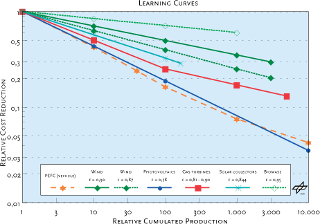
• Production costs tend to decrease with cumulative production capacity, following a so-called learning curve, a logarithmic curve typically described by a learning factor, which is the cost reduction achievable by doubling the cumulative production. The learning factor, which tends to be fairly stable for each specific technology (see figure 4.2), is typically between 0.9 and 0.75, meaning a cost reduction of 10-25% when doubling cumulative production. More innovative technologies tend to have the lowest learning factors (largest cost reductions) compared to more established technologies (cf. also figure 4.2), which also implies that the learning factor does change when seen over very long time horizons. The learning curves for cost reductions mainly reflect savings in manpower, but physical efficiency improvements also play a role. Conservative learning factors (i.e. 0.85 - 0.95) may therefore be used as proxies for the physical flows in a life cycle study when the physical efficiency improvements in these flows are not known from other sources.

Figure 4.2 Learning curves for selected energy technologies. From M. Pehnt: Life Cycle Assessment of Fuel Cells in the Energy and Transportation Sector. Dissertation to be published in summer 2001, Institute for Technical Thermodynamics, German Aerospace Center, Stuttgart

Sources of time series may be:

• Technical literature and technical experts re. the process in question.
• Statistics of industrial associations.
• General statistical publications.

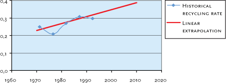
Figure 4.3 shows a simple linear extrapolation of a time series of aluminium recycling rates. The recycling rates are extrapolated by dividing the secondary production of a metal with the primary production. Since recycling rates are influenced by many different conditions, both technical and political, this may be an example of an area where simple extrapolations may not be valid beyond a few years.

Figure 4.3 Simple linear extrapolation of the recycling rate of aluminium

As shown by example 18 an extrapolation is not necessarily quantitative, but can be e.g. a text description of the consequences of extending the prevailing trends into the future.

Limitations of extrapolation in forecasting
Since extrapolation is based on historical data alone, and does not include combined effects of several developments, it can only be used for medium or short-term forecasts for smaller, specific areas, where no radical or untypical developments are expected.

In spite of its limitations, an extrapolation is a better forecast than an assumption of status-quo. Thus, even when there is no time or resources to involve technical experts, it may be justified that a non-expert makes a simple extrapolation as a first approximation.

| Front page | | Contents | | Previous | | Next | | Top |

Version 1.0 December 2005, © Danish Environmental Protection Agency