Effects of Mechanical Weed Control in Spring Cereals – Flora, Fauna and Economy
2 Methods
- 2.1 Study sites and general design of the field study
- 2.2 Weeds and arthropods
- 2.3 Birds
- 2.4 Weed control
- 2.5 Statistical methods and modelling
2.1 Study sites and general design of the field study
The study was carried out in 2004 and 2005 in organic fields that were spring-sown with wheat (Triticum aestivum L.). In both years, six farms located on Zealand, Denmark (Figure 2.1) were used for the study. Two of the farms (Asnæsgård and Viskingegård) were located on Northwestern Zealand, Denmark, another two (Vibygård SØ, Vibygård NV) on Eastern Zealand and the remaining two farms (Oremandsgård and Gl. Oremandsgård) were located on Southeastern Zealand (Figure 2.1, Table 2.1). All study farms were situated on rather clayish soils, which are common in most of Eastern Denmark.
Figure 2.1. Mapped locations of the six study farms in Zealand in Denmark.
A spring-sown crop as selected as the experimental crop because spring-sown cereals are the crops favoured by one of the main study species, the Skylark Alauda arvensis. Spring-sown wheat was preferred to barley and other spring crops because the current trend in Danish organic farming is towards wheat.
In both years the six host farms contributed one field each, yielding a total of 12 experimental fields. In each field, two adjacent plots of approximately equal size (preferably 6 ha and rectangular, in practice 5 to 8 ha and of varying shape) were demarcated, thus retaining the same basic design as in previous studies (Esbjerg & Petersen 2002, Navntoft et al. 2003). This plot size made it probable that a sufficient number of Skylark nests could be found. All plots were placed some distance away from hedgerows and coverts, in an attempt to ensure equal risk of nest predation across plots (within each field).
In each field, the two plots were randomly allocated to one of two different treatments: 2 weed harrowings and 4 weed harrowings. At each farm, the first two harrowings were performed on the same days in “2 harrowings” and “4 harrowings” plots. The first harrowing was carried out before or coinciding with the emergence of the wheat, while the second harrowing was carried out after crop emergence. After that, “4 harrowings” plots were harrowed two times more while “2 harrowings” plots were left untreated. The timing of weed harrowing and other farming operations was the individual farmer’s decision (Table 2.1). The growth stage intervals for the timing of the four weed harrowings were 09, 12-22, 13-31 and 22-46, respectively (decimal code by Tottman & Broad 1987). No restrictions were placed on the farmer with respect to cultivation of the experimental fields before the experiments, previous crop, wheat variety, sowing date, fertilizer use etc.
Table 2.1. The location of the experimental farms and timing of sowing and harrowing.
| Farm | Co-ordinates | Sowing | Weed harrowing | ||||||||||||
| (wgs84) | First | Second | Third | Fourth | |||||||||||
| 04 | 05 | 04 | 05 | 04 | 05 | 04 | 05 | 04 | 05 | ||||||
| Asnæsgård | 55° 39' 48" N; 10° 57' 18" E |
12/4 | 3/4 | 21/4 | 20/4 | 28/4 | 6/5 | 10/5 | 20/5 | 19/5 | 30/5 | ||||
| Viskingegård | 55° 39' 30" N; 11° 14' 42" E |
12/4 | 16/4 | 19/4 | 22/4 | 24/4 | 5/5 | 11/5 | 18/5 | 30/5 | 9/6 | ||||
| Vibygård SØ* | 55° 33' 46" N; 12° 01' 22" E |
13/4 | 3/4 | 21/4 | 18/4 | 12/5 | 13/5 | 28/5 | 26/5 | 8/6 | 10/6 | ||||
| Vibygård NV* | 55° 33' 46" N; 12° 01' 22" E |
15/4 | 4/4 | 23/4 | 18/4 | 14/5 | 14/5 | 1/6 | 20/5 | 8/6 | 26/5 | ||||
| Oremandsgård | 55° 04' 10" N; 12° 03' 53" E |
17/4 | 12/4 | 22/4 | 25/4 | 11/5 | 17/5 | 18/5 | 25/5 | 26/5 | 9/6 | ||||
| Gl. Oremandsgård | 55° 04' 47" N; 12° 06' 18" E |
18/4 | 13/4 | 22/4 | 25/4 | 11/5 | 13/5 | 18/5 | 19/5 | 26/5 | 25/5 | ||||
*Distinct parts of the same holding; co-ordinates denote location of main building
Additional ornithological studies were carried out in a number of fields at one of the farms (Vibygård) in 2006. The crops involved and the farming operations carried out are described in section 2.3.2 below.
2.2 Weeds and arthropods
2.2.1 Field study
Sampling was restricted to the main crop area. Plot margins of minimum 20 m from the field edge were excluded in order to minimise interference between plots and field edges. Within each plot, 11 subplots of 100 m² were selected for sampling (Figure 2.2). For each subplot, the distance to the nearest field margin or other perennial vegetation was measured using GPS. The 11 sub-plots were distributed evenly along the tramlines where the sampling equipment was transported in order to reduce crop damage. Each sample from a subplot comprised four subsamples of 0.15 m² circles. Within subplot no 11, five subsamples were collected. In total 45 = 10´4 + 5 subsamples were collected per plot.
Effects of weed harrowing were determined by estimating arthropod abundances and vegetation biomass simultaneously in the plots subject to two and four times weed harrowing, respectively. Sampling was carried out within one week after the second, the third and the fourth mechanical weed harrowing.
The soil flooding method was used to obtain density estimates of each species of arthropods. The method is described by Brenøe (1987) and Basedow et al. (1988). A 25 cm high circular tube with cross section 0.15 m² (equals one sub sample) was quickly inserted approximately 10 cm into the soil. The above ground vegetation was immediately harvested by cutting and separated into four plant biomass groups: wheat, undersown crop, perennial weed species and annual weed species. While cutting the vegetation all visible arthropods were collected and transferred to 70% alcohol. Immediately after the vegetation was collected the tube was filled with water (approximately 5 l) and all emerging arthropods were collected from the surface. Another 5 l of water was added and the upper soil layer and water was mixed and stirred in order to extract remaining arthropods.
In 2004 the soil flooding method was supplemented with pin point analyses to estimate vegetation cover and pitfall trapping to sample epigaeic arthropod predators. It was decided to use two sampling methods in order to clarify which one was the most efficient and therefore should be the final choice.
Pin point analysis was done with a 1 ´ 1 m² frame equipped with a 10 cm thread mesh, giving 100 intersection points. At each point, a 3 mm Ø pin was inserted vertically, and the plant hit was recorded. The pin point frequency in percent equals number of hits per frame (0-100). The pin point frequency is correlated with cover. One frame per each of the 11 subplots was analyzed. The pin-point analyses were done shortly after 2nd and 4th harrowing in all fields, and only 2004.
Pitfall trapping was carried out using 20 pitfalls placed within each plot as presented in Figure 2.2. The traps were placed approximately 1.5 m from the soil flooding spots. Each trap consisted of a plastic container (diameter 92 mm, depth 80 mm) partly filled with 200 ml of trapping and preservation fluid (a mixture of 1:1 ethylene glycol and tap water, with one drop of nonperfumed detergent per 10 l). A flat roof (20 cm x 20 cm) was placed 15 cm above each of the pitfalls to protect them from rainfall and from predation from birds. The traps were put in the field within a few days after the 2nd, 3rd and 4th weed harrowing and within three to seven days thereafter the traps were collected, labelled and placed in a cold storage until sorting.
Figure 2.2. Schematic diagram of the sampling design in a single experimental field. Pitfall sampling was carried out in 2004 only. Each plot was minimum 6 ha. Arrows indicate tramlines.
In the laboratory, the vegetation samples were dried at 80oC for at least 48 hours, kept at 18-20 oC and weighed. The arthropods were identified under binocular microscope at 5 - 40 x magnification. Araneae were identified at minimum to family following Roberts (1985-1993, 1995). Carabidae were identified to species following Lindroth (1985, 1986) and Staphylinidae were identified to sub-family or more detailed level following Hansen (1951, 1952, 1954). Other arthropods were identified at minimum to order. The scientific, English and Danish names of the organisms studied are presented in Appendix A.
Loooking at the individual weed species the occurring weed species in one the 0.15 m² circles (subsamples) was cut off at soil level and the above-ground biomass of each species was transferred to separate paper bags to determine the dry biomass for each species. The biomass in g dry matter of each species pr subsample was weighed after two, three and four times weed harrowing respectively as describes previously. In total, 81 sampling units were used, of which 65 were determined to species level. In some cases, only genus level determination was possible. Taxonomy according to Hansen (1981).
In august 2004 and 2005 weed phenology was studied. The flowering and diversity of weed species was investigated in 10 of the 11 subplots for each treatment. At each subplot the occurring weed plants, in 2 squares at 0.25 m² each, were determined and classified into one of the following growthstages: seedlings (seed leaves present and less than 5 leaves developed), vegetative plants (no seed leaves present and no flower bud, flower or seed present on the plant), flowering plants (flower bud, flower or immature seeds present) and seedsetting plants (plant with mature seeds or plant that has dropped the seeds).
Species diversity for the weed flora is given by species density (number of species at a given area).
Frequency of flowering is the number of flowering or seed setting weed plants in a square divided by the total number of weed plants in the square.
2.2.2 Field arena experiments
Choice-experiments with carabids placed within steel frames in the field were carried out in order to investigate the indirect effects of weed harrowing measured as the animals preference for weeded and un-weeded ground. The field arena experiments were selected for the reason that results were closer to natural conditions than laboratory experiments as the field provides natural light, humidity and soil conditions, hiding places and natural plant canopy. It was investigated whether the two carabid species Anchomenus dorsalis (Pontoppidan) (subgenus under the genus Agonum) and Bembidion lampros (Herbst) preferred weed harrowed or non-harrowed field.
The experiments were carried out in 2006 and located within a 4 ha South-Eastern corner of a 43 ha large field on Vibygård SØ (Figure 2.3). Against East the experimental area was bordered by a road with a 5 m grass verge in between. Against South the field was bordered by a 20 m wide set-aside area covered with grass and various herbs. The soil was sandy-clay and the crop was spring wheat (cv. Fiorina sown 14 April). Just prior to crop emergence 23 April, the entire field was weed harrowed. Another weed harrowing was carried out 26 May but this time the harrowing excluded the 24 m wide headland.
Figure 2.3. Illustration of the field arena experiments in the South-Eastern corner of an organic spring wheat field. The area was approximately 200 ´ 200 m². Two experiments were carried out, one from 3 - 5 June and one from 9 - 11 June. For the first experiment transects 1, 2, 4 and 5 were used and for the second experiments, transects 3, 4 and 6 were used. The steel frames were placed in such a way that the transects separated the area within the frames in halves with undisturbed soil and vegetation in one half and newly weed harrowed soil in the other half. For each experiment 100 frames were used.
The field arena experiment was carried out twice; the first time from the 3 - 5 June and then again from 9-11 June. At this time the crop was 30 – 40 cm high and GS 32 - 33 (Tottman and Broad 1987).
3 June the headland within the experimental area was weed harrowed, however in such a way that a 2 m wide strip of the headland was left un-harrowed (Figure 2.3). This strip was created by lifting one of middle sections of the harrow (Einbock Aerostar®, 24 m wide harrow from 2002) during operation. The weed harrowing was carried out on slightly humid soil at 7 km/hr and at a pressure of 60 bar, leaving lines with fairly sharp boarders between the weeded an un-weeded soil (four transects).
The steel frames themselves (diam 43 cm, ht 10 cm) caused some shading within the arenas, especially when the sun was at a low angle on the horizon, which could affect the behaviour of the beetles. Different orientations of the transects and the different orientation of weeded and un-weeded soil between transects, secured randomly light intensity between weeded and un-harrowed parts within the arenas, thereby avoiding the introduction of systematic errors in the experimental design.Two of the transects (no. 1 and 2) were running North - South and two were running East – West no. 3 and 4) (Figure 2.3).
4 June, 100 frames were evenly distributed along the transects and placed in such a way, that one half of each arena was covering the weed harrowed field and the other half was covering undisturbed ground. Transect 3 however, had such a poor quality that we considered it unusable for the experiment due to little differences between the weed harrowed and un-harrowed fields. This was caused by unevenness of the ground being an obstacle of efficient weed harrowing. Instead another transect (no. 5) was chosen for the experiment (Figure 2.3). This transect was created by the outer section of harrow.
Not all parts of a transect used were suitable for the choice experiments. Consequently the frames were put in spots selected with the criteria that the harrow had created a clear difference between harrowed and un-harrowed field with a relatively sharp boarder. The frames were forced 5 – 6 cm into the soil leaving 4 - 5 cm above the soil level. On the inside of each arena the upper 5 cm was covered by smooth tape (tesa®) in order to prevent beetles from escaping.
After the establishment of the frames in the field 5 June, each arena was gently searched for naturally occurring beetles, which were removed. Following that, one A. dorsalis and one B. lampros was put in the middle of each arena between 4.30 and 5.30 p.m. The beetles had been marked the previous day with pink fluorescent powder (product from Sun Chemicals A/S), making it possible to trace the beetles in darkness and to distinguish the experimental beetles from possible naturally occurring individuals. The experimental beetles were collected in various organic fields in Eastern Zealand between 24 April and 16 May, using aspirators or pitfalls, which were emptied on daily basis. The beetles were kept in polyethylene boxes (22 x 17 x 6 cm³) with a bottom of slightly humid sand and stored in a refrigerator without food and light at 5°C until use.
Between 11 pm and 0.30 am the beetles were traced within the arenas with as little disturbance as possible using UV-lamps (UNIROSS Lightpower CH8858) and their position recorded (weeded or un-weeded location) (Figure 2.4).
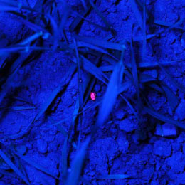
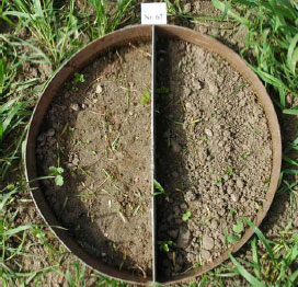
Figure 2.4. Left picture: night photo of an A. dorsalis marked with fluorescent powder and exposed to UV-light. Right picture: steel frame no. 67, 5. June. Undisturbed soil is to the left and weed harrowed soil to the right.
The following day (5 June between 8 am and 10 pm) the position of the beetles within the arenas were recorded again in random order using the following procedure: first a 43 cm x 10 cm steel plate was forced into the ground within the arena, thereby separating the frame in a weeded and an un-weeded half (Figure 2.4). The plate prevented movements of the beetles from one half to the other during inspection. After a brief search for beetles the vegetation from each half was excised at ground level and collected. The biomasses from the weeded and un-weeded halfs were kept apart, separated into weeds and crop and put in paper bags for later biomass estimation using the same procedure as described for the field experiment. Simultaneously with this operation all B. lampros and A. dorsalis seen were collected. Thereafter the upper soil layer was searched for beetles. If the beetles could still not be found, water was added to the arena in order to extract remaining beetles as described for the field experiment (section 2.2.1). All beetles looking like the two experimental species were collected, numbered and their position was recorded together with the name of the finder and the time they were found. They were placed individually in small labelled polyethylene chambers and brought to the laboratory for further species identification and for tracing the marked beetles.
The weather from 3 - 5 June was unstable ranging from dry and sunny to windy with a few showers. The temperatures were 10-20°C. Due to the unstable weather conditions, which were anticipated to have a strong influence on the beetle behaviour, it was decided to repeat the experiment the following week.
9 June a new weed harrowing was carried out, which extended the transects 3 and 4 against West and created a new transect (no. 6) along a gap which had been left untouched by the previous weed harrowing 26 May (Figure 2.3). An attempt was made to harrow transects 1 and 2 again, but we found the result unsuitable for the experiment. The soil was dry and it was weeded with a speed of 10 km/h and at a pressure of 100 - 125 bar. 10 June the 100 frames were placed on transects 3, 4 and 6 on appropriate positions which had not been used before, and following the procedure described previously. No attempt was made to remove naturally occurring beetles from within the frames. Following that, one A. dorsalis was put in the centre of each arena between 2 – 3 pm. The beetles were not marked with fluorescent powder because night observations were omitted from the experiment and because of the risk that it would affect beetle behaviour inappropriately. Furthermore it was decided to include naturally occurring beetles in the experiment. No B. lampros was put artificially as we decided to rely on naturally occurring beetles based on the experience from the earlier study. The vegetation was harvested roughly within the arenas to enhance the chance of finding the beetles but no attempt was made to collect and quantify it because it would become too time consuming. On 11 June between 9.30 am and 10 pm the position of the beetles (harrowed or non-harrowed ground) were recorded as described previously, with the exceptions that this time the arenas were sampled in chronological order to save time and that all arenas were floated to make the experimental condition more uniformly.
The weather from 9 - 11 June was stable with sunshine and light wind. 9 June the day temperature ranged from 15-20°C. 10 and 11 June the day temperatures were between 20-25°C.
2.3 Birds
2.3.1 Skylark
On all experimental fields, nests were searched in 2004 and 2005. The search for Skylark nests on a field began a few days after emergence of the crop, i.e. between 26 April and 4 May (or 13 to 23 days after the field was sown), when the tramlines were just discernible.
Following the recommendations of Odderskær et al. (1997), nest searches were performed using a 4WD vehicle as a hide. While driving up and down the tramlines at low speed (10-15 km/h), the driver and a co-observer constantly looked out for Skylarks. The distance between tramlines varied between fields (12, 18 or 24 m), depending on the equipment used. Whenever a lark was seen rising from the field within 10-20 m of the vehicle, the area from where the bird was flushed was searched by the observers. Also, if a Skylark was seen carrying food or nest material in its bill or showing other signs of nesting behaviour, the car was stopped and the bird was followed using binoculars. At each visit the field was driven through twice, in opposite directions.
As soon as a Skylark nest was found, its location was recorded using GPS
and the site was (in 2004) also marked with two sticks placed c. 5 and 10 m from the nest. This way of marking was used to avoid attracting predators to the nest. However, the nests sometimes proved difficult to re-locate for the observers if the weed cover was dense, increasing search time and vegetation trampling and thus perhaps increasing the risk of predation. Therefore, in 2005 two more sticks (placed so that the two rows of sticks intersected each other at the nest) were used to mark each nest. As there were many other sticks placed in the experimental fields (cf. section 2.2.1), we believe that the marking of nest locations did not attract predators to the nests.
Each field was visited at 4 to 5 day intervals and, in addition to this, after each weed harrowing. At each visit to a nest, its stage was recorded (nest cup without/with complete lining, eggs, young) and the number of eggs and young (alive/dead) in the nest was noted. Age of nestlings was estimated from their size and plumage development. In cases where the age of the young was known (because the nest was visited at time of hatching) it was possible to calibrate our estimation of nestling age at later visits. We believe from these calibrations that our estimations of age, and thus of the day of hatching, were accurate ± 1 day.
Skylark eggs are laid at the rate of one per day, usually early in the morning (Donald 2004). If a nest was found with an incomplete clutch, the date of laying of the 1st egg was therefore known exactly. Also, if a nest was found during nest-building but contained eggs at the next visit, the date of 1st egg could usually be accurately estimated. Incubation generally begins with the laying of the last egg (Cramp 1988, Donald 2004) and the normal incubation time is 11 days (Cramp 1988), although it may vary between 10 and 13 days (Donald 2004). Based on these figures and on the estimations of nestling age, date of 1st egg and start of incubation were estimated in those cases where a nest was discovered with a complete clutch (usually 3 to 5 eggs) or with nestlings.
The young leave the nest while still flightless, usually at an age of 8-10 days (Cramp 1988). Nests containing live young at the last visit before day 8 after hatching and found empty at the next visit (day 8 or later) were classified as successful unless there were clear signs of predation (such as scraped out nest material) or other causes of nest failure. In case of nest failure, the cause was noted (predated, destroyed by weed harrowing, flooded, abandoned etc.). No attempts were made to estimate the survival of chicks after they had left the nest.
The number of visits to each field is shown in Table 2.2. In 2004, the last nest searches were performed on 26 June, with later visits being restricted to controls of previously found nests. In 2005, nests searches continued until 21 July (with later controls of nests), allowing second broods to be included. The stopping of the nest searches in July 2005 coincided with a clear decline in Skylark activity on the fields.
Table 2.2. The number and timing of field visits with searches or controls of Skylark nests in 2004 and 2005.
| Farm | 2004 | 2005 | ||
| Period | No. of visits | Period | No. of visits | |
| Asnæsgård | 29.04 – 25.06 | 12 | 02.05 – 20.07 2) | 19 2) |
| Gl. Oremandsgård | 04.05 – 22.06 | 8 1) | 03.05 – 17.07 | 16 |
| Oremandsgård | 04.05 – 07.07 | 15 | 04.05 – 21.07 | 18 |
| Vibygård NV | 28.04 – 28.06 | 18 | 26.04 – 31.07 | 23 |
| Vibygård SØ | 28.04 – 10.07 | 18 | 26.04 – 23.07 | 22 |
| Viskingegård | 29.04 – 30.06 | 12 | 02.05 – 20.07 | 18 |
1) Number of visits reduced because no signs of Skylark breeding were observed
2) A change of study field was rendered necessary on 17 May (after 4 visits) due to a mistake in the experimental harrowings
The variation between fields in tramline distance (12, 18 or 24 m) possibly affected the probability of nest detection. However, tramline distance and number of visits did not vary between plots within a field. Therefore, the number of nests and the estimates of nest success rate are comparable between treatments, but not between fields or years.
2.3.2 Lapwing and Oystercatcher
In 2004, two of the experimental fields (Oremandsgård and Vibygård NV) held breeding Lapwing (at least 6 and 5 pairs, respectively). Because Lapwing nests were also supposed to be vulnerable to mechanical weed control, and the incubating birds were fairly easily seen in the low vegetation, it was decided to include the species in the study. Thus, Lapwing nests were recorded and marked in the same way as the Skylark nests.
In 2005, searches for Lapwing nests were included from the outset and were also performed (by scanning the fields with binoculars) at a number of exploratory farm visits between 13 and 22 April. Nest locations were GPS recorded and marked with two sticks, as in 2004.
In 2006, a dedicated study of the effect of farming operations on Lapwing breeding success was carried out on a single farm (Vibygård). Four crop types were included:
- Permanent grass – no treatments
- 2nd year grass/clover – no treatments
- Spring cereals with undersown grass – ploughing, sowing and rolling performed but no weed harrowing
- Spring cereals – ploughing, sowing and 3 weed harrowings performed
The experimental fields and the farming operations carried out in 2006 are described in Table 2.3. The oat fields were lying as harrowed stubble until ploughing.
Table 2.3. Fields on Vibygård used for Lapwing studies in 2006 and the dates of the farming operations carried out on each field.
| Field ID Crop Size |
8-1 Permanent grass c. 6 ha |
1-2 2nd year grass/clover c. 20 ha |
4 Spring oats with undersown grass 57 ha |
5+6 Spring oats 21 ha |
95 Spring oats 9 ha |
| Coarse rolling | – | – | 18.04 | – | – |
| Liquid manure spread | – | – | 21.04 | – | – |
| Ploughing | – | – | 22.04 | 11-12.04 | 12-15.04 |
| Harrowing | – | – | 23.04 | 16.04 | 16.04 |
| Sowing | – | – | 24.04 | 18.04 | 18.04 |
| Rolling | – | – | 29.04 | – | – |
| 1st weed harrowing 1) | – | – | – | 28.04 | 28.04 |
| 2nd weed harrowing 2) | – | – | – | 03.05 | 03.05 |
| 3rd weed harrowing | – | – | – | 27.05 | 27.05 |
1) Before crop emergence
2) Immediately after crop emergence
The nest searches in 2006 were carried out from a 4WD vehicle as described for Skylark and by scanning the fields from vantage points, using binoculars and telescope (27 x magnification). Nest locations were recorded and marked as in the previous study years. Until 10 May the fields were generally visited at 3 to 4 day intervals, but from mid-May onwards access to some fields was restricted due to hunting interests. The number and timing of visits to each field are shown in Table 2.4.
Table 2.4. The number and timing of field visits with searches or controls of Lapwing nests in 2006.
| Field ID / Crop | 8-1 Permanent grass |
1-2 2nd year grass/clover |
4 Spring oats with undersown grass |
5+6 Spring oats |
95 Spring oats |
| Period | 07.04 – 10.05 1) | 07.04 – 27.05 2) | 07.04 – 08.06 | 07.04 – 31.05 3) | 07.04 – 31.05 |
| No. of visits | 10 1) | 14 | 15 | 11 | 13 |
1) Period curtailed to avoid conflicts with hunting interests
2) Only nest controls (no nest searches) after 15 May
3) Visits after 15 May limited to two nest controls (27 and 31 May)
Date of 1st egg and start of incubation were estimated using the following information: Lapwing eggs are laid with an interval of c. 36 hours, implying that a clutch of four eggs (85-90% of clutches) is normally completed on day 5 after the laying of the first egg (Cramp & Simmons 1983). Incubation begins with the last egg, but earlier eggs are covered intermittently, especially in bad weather. Different authors cited by Cramp & Simmons (1983) state incubation times ranging from 21 to 28.1 days; in the present study we found incubation times of 25-26 days in those (few) cases where date of clutch completion as well as date of hatching were known. A standard incubation time of 25 days was used to estimate the date of clutch completion and/or hatching date. A similar incubation time was used by Galbraith (1988).
Lapwing chicks are precocial and usually leave the nest within few hours after hatching. The larger eggshell parts are removed by the adults, whereas the tiny fragments derived from the initial perforation of the egg by the young are left (H. Olsen pers. comm.). These fragments may usually be found by careful inspection of the nest and indicate that hatching has occurred. If such fragments could not be found, a nest found empty at the first visit after the estimated date of hatching was only classified as successful if anxious adults were nearby (indicating the presence of chicks) or if the eggs had actually been in the process of hatching at the previous visit. In case of nest failure, the cause was noted (predated, destroyed by farming operations, abandoned).
The chicks may move far away from the nest and no attempts to estimate chick survival were made.
In addition to the Lapwing nests, a few nests of Oystercatcher Haematopus ostralegus were found in 2004 and 2005. These nests were marked and monitored like the Lapwing nests. In the Oystercatcher, the most frequent clutch size is 3, the eggs are laid at a rate of one per day and the normal incubation time is 27 days (Cramp & Simmons 1983, van Oers et al. 2002). However, in one successful nest monitored in 2004, incubation time was at least 28-29 days.
The data on Lapwing and Oystercatcher nests that were collected during the present project were supplemented with data from Kalø Estate, East Jutland (56º18’N, 10º30’E), collected as part of the project “Ukrudtsstriglingens effekter på dyr, planter og ressourceforbrug” (Odderskær et al. 2006). In the Kalø project, two fields (27 and 35 ha, respectively) sown with spring wheat in 2004 and 2005 were divided into two plots of equal size. One of the plots in each field received 3 weed harrowings (performed after emergence of the crop, between 17 and 38 days after sowing) while the other plot was left untreated. The fate of the Lapwing and Oystercatcher nests found on these fields was recorded in the same way as in the present project.
2.3.3 Data analysis
The major causes of nest failure on the study fields were farming operations (first of all weed harrowing) and predation. Nests were classified as failed if no young left the nest, while nests where at least one young left the nest were classified as successful. For calculation of nest and egg loss rates caused by weed harrowing, only nests that were known and active at the last visit before a harrowing event were used. In a few cases, a previously unknown nest was found after weed harrowing with the age of the nest indicating that it had survived the harrowing. These nests were not included in the calculation of loss and survival rates in relation to harrowing because unknown nests that do not survive harrowing will not be discovered afterwards. Loss/survival rates were calculated simply as the number of nests or eggs destroyed/partially destroyed/intact divided by the number of monitored nests or eggs.
Contrary to nest losses caused by farming operations, predation losses may occur any day a nest is active. Simple calculations of predation frequency (no. of known nests predated / no. of known nests) underestimate the frequency of predation, because a number of nests may be predated before they are found, especially if predation rates are high. Therefore, mean daily predation rates were calculated by dividing the number of nests predated by the number of days the nests were monitored (nest-days). The frequency of predation was then estimated from the formula 1 – (1 – P)n where P is the daily predation rate and n is the mean number of days from the first egg is laid until the young leave the nest (put at 23 days in Skylark and 30 days in Lapwing and Oystercatcher). The formula assumes P to be constant throughout the nest cycle. Especially in the Skylark this may be an oversimplification, but data did not allow separate estimation of daily predation rates during incubation and chick-feeding.
2.4 Weed control
Three types of “Landsforsøg” trials have been selected to describe the economy and the weed control effect of chemical and mechanical weed control in spring barley. The three describe the effect of 1) An increased number of weed harrowings in organically grown spring barley, 2) Chemical and mechanical weed control strategies in conventionally grown spring barley, and 3) Barley varieties, seed density and chemical weed control in spring barley.
The trial designs, treatments, field registrations and results can be found on the homepage of Danish Agricultural Advisory Service: http://www.lr.dk, and some of the results are reported and discussed in Petersen (2002, page 121+122, 123+124 and 241+242). Each trial has a table number, a Danish title and a unique series number. The series number can be used to access the series’ electronic data storage. For instance data on series 091970101 can be found on http://www.lr.dk/dbmf/tabelbilag/0919701.html.
2.4.1 Data for an increased number of post-emergence harrowings
To analyse the economy and weed control effect of an increased number of harrowings in spring barely, 8 national trials from 2001 and 2002 are selected.
Table H36. Increased number of weed harrowings in organically grown spring barley, 2001 and 2002. Series 020280202, 020280101, 091970101, 091990202.
http://www.lr.dk/dbmf/tabelbilag/0242802.html
1. Untreated
2. Pre-emergence harrowing 5 days and post-emergence harrowing 7 days after sowing.
3. Pre-emergence harrowing 5 days and post-emergence harrowing 7 + 14 days after sowing.
4. Pre-emergence harrowing 5 days and post-emergence harrowing 7 + 14 + 21 days after sowing.
5. Pre-emergence harrowing 5 days and post-emergence harrowing 7 + 14 + 21 + 28 days after sowing.
2.4.2 Data on chemical and mechanical weed control strategies
To analyse the economy and weed control effects of different weed control strategies, including chemical (use of pesticides) and mechanical (pre and post crop emergence harrowing) weed control, 32 national trials (Petersen 2005) with mechanical and so-called chemi-chanical (kemikaniske) treatments are selected. The trials are performed in the period from 1999 to 2002 using more than three different designs, each involving five to eight treatments. But all of the trials include an untreated reference treatment, a treatment with a proper (full, half or optimal) dose of herbicides, and a treatment combining a pre and a post emerge harrowing. The rest of the two to five treatments per site are focusing on timing and number of treatments as well as combinations of low herbicide doses and pre or post emergence harrowing.
Table C36. Weed harrowing in spring barley. Series 092129999 http://www.lr.dk/dbmf/tabelbilag/0921299.html
1. No weed control
2. St. 11-12 PC-Plant protection, weed + 50 % Recommended dosage
3. St. 11-12 PC-Plant protection, weed + 25 % Recommended dosage
4. St. 08: Weed harrrowing, St. 11-12 PC-Plant protection weed + 50 % Recommended dosage
5. St. 08: Weed harrrowing, St. 11-12 PC-Plant prtotection, weed + 25 % Recommended dosage
6. St. 08 Weed harrrowing
7. St. 08 Weed harrrowing, St. 12-13 Weed harrrowing
Table C35. Weed harrowing in spring barley. Series 091910000.
http://www.lr.dk/dbmf/tabelbilag/0919100.html
1. No weed control
2. St. 11-12 PC-Plant protection, weed + 50 % Recommended dosage
3. St. 11-12 PC-Plant protection , weed + 25 % Recommended dosage
4. St. 08: Weed harrowing, St. 11-12 PC-Plant protection ukr. + 50 % Recommended dosage
5. St. 08Weed harrowing, St. 11-12 PC-Plant protection ukr. + 25 % Recommended dosage
6. St. 08 Weed harrowing
7. St. 08 Weed harrowing, St. 12-13 Weed harrowing
8. St. 08 Weed harrowing, St. 12-13 Weed harrowing, St. 12-13 + 7 days Weed harrowing
Table C35. Increased number of weed harrowings in organically grown spring barley. Series 091970101, 020280101.
http://www.lr.dk/dbmf/tabelbilag/0919701.html
1. No harrowing
2. 5 days after sowing Harrowing, 7 days after sowing Harrowing
3. 5 days after sowing Harrowing, 7 days after sowing Harrowing, 14 days after sowing Harrowing
4. 5 days after sowing Harrowing, 7 days after sowing Harrwoing, 14 days after sowing Harvning, 21 days after sowing Harrowng
5. 5 days after sowing Harrowing, 7 days after sowing Harrowing, 14 days after sowing Harrowing, 21 days after sowing Harrowing, 28 days after sowing Harrowing
6 Weed maximum 4 leaf stage 2 tb Express + 0.1 l Lissapol Bio
Table C33. “Chemi-chanical” weed control in spring barley. Series 092010101
http://www.lr.dk/dbmf/tabelbilag/0920101.html
1. No weed control.
2. St. 11-12: PC-Plant protection, weed + Recommended dosage
3. St. 08: Pre-emergence harrowing St. 11-12 PC-Plant protection weed + Recommended dosage
4. St. 08: Pre-emergence harrowing, St. 12-14 Weed harrowing
5. St. 11-12: Chemi-chanical PC-Plv. + Recommended, 5-7 days after spraying weed harrowing
6. St. 11-12: Chemi-chanical PC-Plv. + Recommended, 16-18 days after spraying weed harrowing
Table C34. Chemi-chanical weed control in spring barley. Series 092020101
http://www.lr.dk/dbmf/tabelbilag/0920201.html
1. No weed control.
2. St. 11-12: PC-Plant protection, weed + Recommended dosage
3. St. 11-12: Chemi-chanical PC-Plp. + 50 % REcommended dosage, 8-10 days after spraying Weed harrowing
4. St. 11-12: Chemi-chanical PC-Plp. + Recommended, 8-10 days after spraying Weed harrowing
5. St. 11-12: Chemi-chanical PC-Plp. + 200 % Recommended dosage, 8-10 days after spraying Weed harrowing
6. St. 08: Pre-emergence harrowing, St. 21-25 Weed harrowing
Table C36. Chemi-chanical weed control in spring barley Series 091960202.
http://www.lr.dk/dbmf/tabelbilag/0919602.html
1. No weed control
2. St. 11-12: PC-Plant protection, weed + Recommended dosage
3. St. 08: Pre-emergence harrowing, St. 11-12: PC-Plant protection, weed + Recommended dosage
4. St. 08: Pre-emergence harrowing, St. 12-14: Weed harrowing
5. St. 11-12: Chemi-chanical PC-Plp. + Recommended dosage, 5-7 days after spraying Weed harrowing
6. St. 11-12: Chemi-chanical PC-Plp. + Recommended dosage, 16-18 days after weed spraying Weed harrowing
7. St. 11-12: 0.5 ta Express + 0.25 l Oxitril CM
Table C37. Chemi-chanical weed control in spring barley. Series 091970202.
http://www.lr.dk/dbmf/tabelbilag/0919702.html
1. No weed control
2. St. 11-12: PC-Plant protection weed + Recommended dosage
3. St. 11-12: Chemi-chanical PC-Plp. + 50 % Recommended dosage, 8-10 days after spraying Weed harrowing
4. St. 11-12: Chemi-chanical PC-Plp. + Recommended dosage, 8-10 days after spraying Weed harrowing
5. St. 11-12: Chemi-chanical PC-Plp. + 200 % Recommended dosage, 8-10 days after spraying Weed harrowing
6. St. 08: Pre-emergence harrowing, St. 21-25: Weed harrowing
7. St. 11-12: 0.5 ta Express + 0.25 l Oxitril CM
2.4.3 Data on barley varieties and seed densities weed control effect
To analyse the economy and weed control effects of different spring barley varieties and varying seed densities with and without chemical weed control, nine more national trials (Petersen 2005) are selected. The trials were performed on 3 locations in 2001 and 6 locations in 2002 using the same three factors and the 18-treatments design. The spring barely varieties Lux, Jacinta and Otira are supposed to compete less, normally and well with the weed. The 0.4 tablet Express and 0.1 l Oxitril corresponds to a TFI of 0.3 (BI).
Table C39. Spring barley’s competitive advantage over weeds. Series 091910202.
http://www.lr.dk/dbmf/tabelbilag/0919102.html
Table C36. Spring barley’s competitive advantage over weeds. Series 091910101.
http://www.lr.dk/dbmf/tabelbilag/0919101.html
Factor 1 (Variety):
1. Lux
2. Jacinta
3. Otira
Factor 2 (Density):
1. 150 Fit barley seeds per m²
2. 300 Fit barley seeds per m²
3. 450 Fit barley seeds per m²
Factor 3 (Weed control):
A. No weed control
B. Growth stage 11-12 0.4 tablet Express + 0.1 l Oxitril CM + 0.1 l Lissapol Bio
2.5 Statistical methods and modelling
The statistical models used are listed in Table 2.5. In the following the models are described in words whereas the mathematical formulations of the models are given in Appendix C.
Table 2.5. Statistical models used for analysing the recorded data.
| Model number | Applied to | Purpose |
| 1 | Number of weed species and number of hits after 3rd or 4th harrowing in a single year | To estimate and test for effect of farm and two or more harrowings when adjusting for the recording after 2 harrowings |
| 2 | Biomass and arthropods after 3rd or 4th harrowing from all farms in both years | To estimate and test for effect of year, two or more harrowings and their interaction |
| 3 | Arthropods after 3rd or 4th harrowing from all farms in both years | To estimate and test for the effect of distance to perennial vegetation, the effect of crop biomass and weed biomass when adjusting for the effect of year, two or more harrowings, their interaction and recorded arthropods after 2 harrowings |
| 4 | Biomass and arthropods from both harrowings at all farms in both years | To estimate and test for the effect of year, two or more harrowings and time of harrowings together with their 2- and 3-way interactions |
| 5 | Pitfall trapping of arthropods in 2004 | To estimate and test for the effect of farm, two or more harrowings and distance to perennial vegetation when adjusting for the recording after 2 harrowings |
| 6 | Arthropods in 2 harrowing plots at the time of 4th harrowing | To have a model that could be used as a basis (null-model) for comparison with model 7 to estimate a vegetation – arthropod relationship |
| 7 | Arthropods in 2 harrowing plots at the time of 4th harrowing | To estimate and test for the effect of weed biomass, crop biomass and distance to perennial vegetation |
| 8 | Average number of artropods per m² in each field | To estimate and test the effect of weed biomass, crop biomass and distance to perennial vegetation on the number of arthropods |
| 9 | Preferences of two species in the field arena experiments at each of the recordings | To estimate and test the preference for harrowed or non-harrowed soil and the effect of species for A. dorsalis and B. lampros |
| 10 | Preferences of two species in the field arena experiments at each of the recordings | To estimate and test the preference for harrowed or non-harrowed soil, the effect of species together with the effect of some covariates for A. dorsalis and B. lampros |
| 11 | Preferences of two species in the field arena experiments simultaneously for the two day recordings | To estimate and test the preference for harrowed or non-harrowed soil, the effect of day, the effect of species, interaction between species and day together with the effect of time for A. dorsalis and B. lampros |
| 12 | Recorded relative variables for birds | To estimate and test the effect of two or four harrowings on the recorded relative variables |
| 13 | Recorded number of nests, eggs, hatchlings and fledglings | To estimate and test the effect of two or four harrowings on the recorded numbers |
| 14 | Calculated variables per nest day for birds | To estimate and test the effect of two or four harrowings on the variables calculated as nest-days |
2.5.1 Weeds and arthropods
2.5.1.1 Field experiment
For each plot 45 sampling were taken per sampling day. This number was chosen as an analysis based on earlier sampling in organic fields showed that this would yield an acceptable power.
The number of weed species and number of hits in 2004 were analysed in a generalised linear mixed model (see e.g. McGulloch & Searle 2001) where the effect of farm and number of weed harrowings were included as fixed effects. The random effect of weed harrowings on each farm was included as a random effect (model 1).
The weight of each type of biomass was analysed using linear mixed models. The weight of each type of biomass recorded after 2nd, 3rd and 4th weed harrowing were anlysed in a basic model including the effects that were “dictated” by the design, i.e. number of weed harrowings, year, farm, subplot and sub sampling together with relevant interaction (model 2).
There were found several different arthropod taxi, but only four of them were found in sufficient numbers for statistical analysis. That was the spider family Linyphiidae, the rove beetle genus Tachyporus and the two carabid genera Agonum and Bembidion. Each arthropod and sum of arthropods recorded after the 3rd and 4th weed harrowing was analysed using 3 different models. The first, basic model only included the effects that were caused by the design, i.e. number of weed harrowings, year, farm, subplot and sub sampling together with relevant interaction (model 2 - as for weight of biomass). The second model also included covariates in order to describe any possible effects of the number of arthropods after the 2nd weed harrowing, the distance to nearest perennial vegetation, amount of weed and crop in the sub sample (model 3). After fitting model 3 this model was reduced step by step until all remaining effects were significant at the 10% level. The reduced model was used to evaluate how the different type of vegetation and distance to perennial vegetation influenced the number of arthropods. Finally all the recordings from all three sample times were analysed jointly in a model that also included the effect of time and relevant interactions with time for comparisons of effects of 3 and 4 harrowings on polyphagous predators (model 4).
The parameters of these models (and the following models) were estimated using the method of Restricted Maximum Likelihood (REML). Based on the estimates the parameters of interest were calculated as linear functions of the fixed effects mentioned above. Tests were done using F-tests with denumerator according to the theory of mixed models (see McCulloch & Searle 2001) using the principles of Satterthwite (Satterthwite 1946) for calculating the approximate denumerator degrees of freedom. All calculations were done using the SAS procedures glimmix and mixed (SAS Institute Inc. 2005 and 2006).
Pitfall trapping of arthropods in 2004
The data were analysed in a generalised lienar mixed model. The following effects were included in the model: farm weed harrowing, number of arthropods after second weed harrowing and distance to nearest perennial vegetation (model 5).
The relation between weed biomass and weed species composition
The question was whether variation in weed species composition reflects differences in ecological growth conditions between the experimental plots, based on Sørensen similarity and Ellenberg index calculations (Ellenberg 1974, Ellenberg et al. 1991). In total 81 taxons of weed plants were found in the biomass subsamples. In order to calculate Sorensen similarity and weighted Ellenberg indices, the biomass samples were ranked in separate weight classes. The number of intervals was 30, and the total number of biomass samples was 789. The Sørensen similarity index is calculated as
![]()
where a is the number of shared species, b is the number of species only in collection 1, and c is the number of species only in collection 2. See Krebs (1998) for further methods and indices.
Ellenberg indices cover a range of environmental variables of importance to plant growth. The variables are: L: Light; T: Temperature; K: Continentality; F: Humidity; R: pH; N: Available nitrogen. For all observed plants, their position on a scale from 1 to 9 for these 6 categories is taken from published tables based on the present scientific knowledge of the species autecology, and the number multiplied by the chosen importance value, if weighted indices are wanted. If, e.g., the species composition is characterized by a generally high score on the F scale, the analysed site is probably close to a wetland ecosystem. See further in Ellenberg (1974) and Ellenberg et al. (1991).
Vegetation effect on arthropod abundance
In order to exclude any effects caused by the number of harrowings this analysis only include those recordings after 4 weed harrowings from field halfs that were treated with only 2 weed harrowings. Each arthropod taxon (Agonum, Bembidion, Linyphiidae, Tachyporus) and the sum of these were analysed using two different models. The first model only included year as fixed effect (model 6). The second model also included the effect of the number of arthropods after 2nd weed harrowing and distance to nearest perennial vegetation and amount of the two biomass types: crop and weed (model 7). Afterwards the 2nd model was reduced using the same principles as when analysing the data from both weed harrowing (see above).
Estimating a non-linear vegetation-arthropod relationship
In order to estimate a non-linear dependence between biomass and arthropods, the number of arthropods, logarithm of distance to nearest vegetation, amount of crop and of weed was averaged within each field half receiving a maximum of two weed harrowings. (across subplots and sub samples taken after the fourth harrowing) Those averages were used to fit models that described this dependence. The parameters of the model thus depend only on the means recorded in each individual field.
The non-linear mixed model was based on the logistic function and included the effect of distance to perennial vegetation, amount of weed and crop biomass and assumed that an upper bound of arthropods per unit of land exists. The effect of the crop biomass was described relative to the effect of weed (model 8).
2.5.1.2 Field arena experiments
For each assessment 100 frames were used. This number were chosen as power calculations showed that it would be necessary to have about 100 animals in order to be able to decide (at the 5% level of significance) whether there were significance preference for either of the treatments if the true preference were 35%/65%.
The recorded animals were analysed using a generalised linear mixed models that assumed that the preference (probability) of being in the weeded part of the frame was binomial distributed. Three different models were used. The first, basic model only included the effects of weed harrowing and species (model 9). The second model also included covariates in order to describe any possible effects of variables such as biomass (crop and weed) in the two halves and recording time (model 10). However, some covariates were only present at certain recording dates. This model was reduced step by step until all remaining effects were significant at the 10% level. The reduced model was used to evaluate how the different covariates influenced the preferences of the two species. Finally all the recordings from the two day samplings were analysed jointly in a third model that also included the effect of dates and relevant interactions with dates (model 11).
The parameters were estimated and tested using the same statistical methods as described for the field experiment.
2.5.2 Birds
The variables recorded as numbers or relative numbers were analysed in a generalised linear mixed model that took into account the treatment effect and the random effects of year, farm and the combination between year and farm. A possible overdispersion/underdispersion was included in order to take into account any additional random variation between years and between farms (model 12 and 13). The variables calculated per nest-day were analysed in a linear mixed model assuming that the data were normally distributed and with the same effects as mentioned above for numbers and relative numbers (model 14).
2.5.3 Weed control
2.5.3.1 The complex of weed control models
A complex of first and second order models has been established to describe crop yield, crop density, weed density, weed biomass, and yield loss (from harrowing, herbicides and weed) as functions of planned (ex ante) and actual (ex post) weed density, weed plant biomass potential, crop yield potential, crop seed density, crop plant yield/biomass potential, herbicide dose, harrowing intensity, etc. The model complex includes new herbicide response and synergy functions (Ørum, Rydahl & Kudsk 2006), novel use of this new response functions for mechanical weed control (Ørum & Rasmussen 2006), and, inspired by Cousens (1985), the models also include hyperbolic inter- and intra-specific (crop and weed species) competition. The basic hyperbolic inter- and intra-specific (crop and weed species) competition functions are established in close cooperation with the Crop Protection Online (PVO) project (Jørgensen et al. 2007) and with help, inspiration and data from Anne Mette Jensen (University of Copenhagen), Jens Erik Jensen, (Danish Agricultural Advisory Service) and Peter Kryger Jensen, Niels Holst and Karen Henriksen (University of Aarhus, Faculty of Agricultural Sciences). All in all, the model complex is novel and not yet published, and neither University of Aarhus nor Danish Agricultural Advisory Service is responsible for the model complex or the way it is used in this report. The following presentation gives a brief overview of the model complex used.
For each trial and strategy (treatment), the crop density (P), weed density (D), relative crop soil cover (z), and crop yield (Y) has been registered, whereas the weed biomass (W) has not been registered.
A model complex (formula 1-9) has been established in order to calculate the within-trial treatments (i),crop yield (Y), and the weed biomass (W) as a function of planned crop density (P), herbicide dose (x), harrowing intensity (z), potential crop yield (Y), potential (untreated and crop free) weed biomass (W), and conditions for the effect of herbicides and harrowing (α):
Weed biomass:
1) 
Crop yield:
2) 
Formulas 1-2 are the primary functions, whereas formulas 3-4 are used for estimation purposes:
Weed density and biomass:
3) 
Crop density:
4) ![]()
The functions f, g, and h express the harrowing (z) and herbicides’ (x) relative effect (survival) on weed, crop yield and crop density, respectively. Theα represents local (ex post) herbicide and harrowing response parameters. Theω, μ are local (ex post) weed and crop plant weights. And the β, ρ κ λ γ andC are common (ex ante) response slopes, synergy and intra/inter-specific feedback parameters.
Herbicides relative effect (survival) on weed biomass, crop yield and crop density is calculated:
5) 
Harrowing relative effect (survival) on weed biomass, crop yield and crop density is calculated:
6) 
In the case of repeated post emergence harrowing:
7) ![]()
In case of a combination of pre- and post-emergence harrowing:
8) ![]()
In case of a combination of herbicides and post emergence harrowing:
9) ![]()
2.5.3.2 Parameter estimation and testing
Some of the model complex parameters used in formula 1-9 above have been set beforehand or estimated from findings in the literature and DJF trials included in the Crop Protection Online project (Jørgensen et al. 2007), but most of the parameters have been estimated by using the selected 32 + 9 Landsforsøg and non-linear simultaneous regression analysis using weighted least square estimation by means of the Newton-Raphton method.
The beta response parameter βx used to calculate the herbicides’ (x) effect on weed and crop in formula 5 and 9 has been set to 0.6. Experiments in the Jørgensen et al. (2007) project has shown that the beta parameter for the different herbicides varies from 0.57 to 1.33. Express (tribenuron-methyl) and Express + Oxitril (ioxynil and bromoxynil) are the most used herbicides in the 32 + 9 trials. The general beta response parameter for these herbicides has in Jørgensen et al. (2007) been estimated to 0.65 and 0.57, respectively. An additional analysis has shown, that 0.6 is a decent beta parameter for blends of herbicides including herbicides with even higher individual beta parameters.
Also the beta response parameter βz used to calculate the post emergence harrowing (z) effect on weed and crop in formula 5 and 9 has been set to 0.6. Findings from scientific articles on weed response to post emergence harrowing indicate that the harrowing beta varies from 0.53 to 0.84 with an average around 0.58 (Ørum and Rasmussen, 2007).
Modelling the weed biomass and the crop yield as a function of the weed biomass is the main task for the model complex, but unfortunately the weed biomass and the specific weed density has (as always) not been registered in the available Landsforsøg trials with mechanical weed control and barley species. To compensate for this gap, the weed biomass is estimated by using the weed density data plus knowledge and functionality established in the Jorgensen et al. (2007) project. In that project the relation between weed density and weed biomass has been analysed for more than 100 herbicide trials in spring barely, including more than 1.100 treatments and detailed registrations on crop yield and weed species density and biomass.
In the Jørgensen et al. (2007) project, the ρ parameter in formula 3, used to describe the correlation between the reductions in weed density and weed biomass from using herbicides and harrowing, has been estimated to 0.6 for herbicides (ρx). Here it is also found that the observed average untreated weed plant weight (W0/D0) is 5 g per m², and that the estimated average crop-and-weed-free weed plant weight (ω) is 10 g per m² with a 10 g per m² standard deviation.
The rest of the parameters are in principle estimated simultaneously, but in practice the parameters have been estimated in an iterative stepwise process. First the local (ex post) parameters (see table 2.7) are estimated for each location, then the common (ex ante) parameters, all the local parameters, the common parameters plus local crop and weed weights, and the common parameters and the local response parameters (see table 2.6) have been estimated. All these parameters have been estimated again and again until the weighted sum of the squared error terms (εW, εY and εD) from formula 1, 2 and 3 are minimized (stabilized).
Unfortunately none of the selected trials are dealing with sole post emergence harrowing, weed biomass has, as mentioned, not be registered and the harrowing intensities (z) have not been registered in the series 091970101 and 020280101 trials. A crop soil cover from 10 to 20% is recommended in the Landsforsøg trials, but intensity varies from trial to trial, having an average crop soil cover around 10%. If the intensity for the series 091970101 and 020280101 trials are set to high, the average effect of a 20% crop soil cover harrowing is underestimated, and if the crop soil cover is set to low, the average effect of a 20% crop soil cover harrowing is overestimated. According to Rasmussen (2004) and Odderskær et al. (2006), a 20% crop soil cover harrowing is expected to reduce the weed biomass by 70%. Due to the above mentioned shortcomings, the resulting average reduction in weed biomass from a standard harrowing can not be estimated exactly nor calculated from the selected Landsforsøg trials alone. It has been decided to estimate an average crop soil cover between 10 and 20% for the series 091970101 and 020280101 trials yielding an average 70% reduction in case of a 20% crop soil cover harrowing in all 32 trials with weed harrowing. Actually an 8% crop soil cover in the series 091970101 and 020280101 trials is needed to achieve this goal. But in order not to overestimate the weed control effect a 12.5% crop soil cover has been set for the two series, resulting in a 68% average reduction in the weed biomass. If the two missing crop soil covers were set to 5 or 20% the average effect of a 20% crop soil cover would have been 66 and 71% respectively.
Table 2.6 shows the common (ex ante) parameter estimates.
Table 2.6. Common (ex ante) parameter estimates.
| Parameter | Explanation | Weed biomass | Crop yield | Crop density |
| βx | Herbicide response (slope) | 0.6 | ||
| βZ | Harrowing response (slope) | 0.6 | ||
| ρx | How herbicides retard weed | 0.6 | ||
| ρZ | How harrowing retard weed | 0.73 | ||
| κ | Crop influence on weed biomass | 0.045 | ||
| λ | Weed biomass influence on crop | 0.6 | ||
| αYx | Crop damage from herbicides | 0.26 | ||
| C1. 2. 3… | Post x Post synergy | 0.752 | 1.09 | 0.714 |
| Pre x Post synergy | 0.05 | 0.05 | 1.25 | |
| Herbicides x Post synergy | 1.25 | 0.05 | 0.05 | |
| Aux. αp | Alpha factor Pre harrowing | 18% | ||
| Alpha factor Post harrowing | 58% | |||
| Varieties | Lux weight and yield factor | 1 | 1 | |
| Jacinta factors | 0.72 | 1.04 | ||
| Otira factors | 1.4 | 1.02 | ||
| μ | Aux. density factor | 0.973 | ||
Source: Selected Landsforsøg (Petersen, 2006).
In the Crop Protection Online (PVO) decision support system for chemical weed control (Bøjer & Rydahl 2007) used in wide range of arable crops, it is anticipated that each herbicide has only one beta parameter valid for all conditions, weed species and crops. As a parallel to this, it has been decided that also harrowing has only one, general beta response parameter valid for all conditions, weed species and crops.
The ρZ parameter used to describe the correlation between the reductions in weed density and weed biomass from using harrowing has been estimated to 0.73. This value does not differ significantly from the 0.6 found for herbicides (ρx). But, it indicates that weed treated with herbicides are more retarded than weed treated with harrowing, and that weed surviving the harrowing is more vital than weed surviving herbicides.
The synergy parameters C are used to add up the effect of more harrowing or combinations of harrowing and herbicides. According to Ørum et al. (2007), a synergy factor close to 1, like the estimated harrowing plus harrowing synergy effect on the crop yield, indicates that each harrowing is reducing the yield or weed biomass by the same factor (Minimum survival model, MSM), whereas a synergy factor close to 0.6, like the harrowing plus harrowing synergy effect on the crop density, indicates that the herbicide doses and harrowing intensity are additive (Additive dosage model, ADM). In case of a high (higher than 0.6) synergy factor, like the herbicide x post emergence harrowing effect on weed biomass (1.2), the combined effect of a low herbicide dose and a normal post emergence harrowing is supposed to be very effective. And in case of a low synergy factor (below 0.6), like the pre x post emergence harrowing effect (0.15), the weed control effect of a pre-emergence harrowing is almost lost if the pre-emergence harrowing is combined with an effective post emergence harrowing. The 0.7 harrowing x harrowing synergy factor for weed biomass indicates that the effect of splitting up the harrowing is somewhere between MSM and ADM. This could indicate, that ADM is the right model if the exact effects of the harrowings are known, and the better synergy than ADM is due to the fact that for one intensive harrowing with a good or bad timing is on average less effective than two less intensive harrowings having a good and a bad timing. In case of the harrowing x harrowing synergy factor for weed biomass right between MSM and ADM, more analyses are needed to identify the most efficient harrowing strategy.
The auxiliary alpha factors for pre- and post emergence harrowing indicate that harrowing and, especially, pre-emergence harrowing are relatively less damaging to the crop density than to the crop yield. The local pre- and post emergence harrowing alpha response parameters used to calculate the crop yield are also used to calculate the crop density, but multiplied by the auxiliary alpha.
The estimated barley varieties factors indicates, as expected, that the varietis Otira with a 1.4 weight factor is the most competitive of the three varieties, but, the varieties Jacinta and not the variety Lux is found to be the least competitive variety. The yield factors indicate that, on average, Jacinta and Otira offer a 4% and 2% higher yield potential than Lux. In this way Jacinta may still end up being more competitive or less weed depending than Lux.
Table 2.7 shows the local (ex post and stochastic) parameter estimates.
Table 2.7. Local (ex post or stochastic) parameter estimates.
| Parameter | Explanation | Unit | Average | Standard deviation | Average | Standard deviation |
| 32 herbicide and harrowing trials | 9 variety and seed density trials | |||||
| Y | Potential yield | Hkg ha-1 | 63.2 | 11.1 | 59.7 | 13.3 |
| γ | Crop plant weight | Hkg ha-1 | 12.7 | 2.3 | 9.9 | 4.9 |
| ω | Potential weed plant weight | g m-2 | 10.3 | 8.2 | 8.4 | 4.0 |
| P | Observed untreated crop density | m-2 | 242 | 54.5 | 300*) | 150 |
| D0 | Observed untreated weed density | m-2 | 103 | 92 | 241.7 | 54.5 |
| αWx | Herbicide weed response | 3.6 | 2.2 | 4.3 | 2.6 | |
| αWb | Pre-emergence harrowing weed response | 0.85 | 0.60 | |||
| αWz | Post emergence harrowing weed response | 4.8 | 1.9 | |||
| αYB | Pre-emergence harrowing yield response | 0.17 | 0.27 | |||
| αYz | Post emergence harrowing yield response | 1.1 | 0.9 | |||
*) The crop density in the variety and seed density trials are defined as150, 300 and 450 plants per m-2.
Source: Selected Landsforsøg (Petersen, 2006).
Version 1.0 August 2007, © Danish Environmental Protection Agency