Model assessment of reductive dechlorination as a remediation technology for contaminant sources in fractured clay: Case studies
4 Vadsbyvej
- 4.1 Characterization of contamination source
- 4.2 Geological characterization – Fracture distribution
- 4.3 Hydrogeological characterization
- 4.4 Model configurations and scenarios
- 4.5 Modeling results
- 4.6 Sensitivity analysis on parameters
4.1 Characterization of contamination source
The source zone is defined based on the mass distribution calculations performed by the consulting company Orbicon. The concentration measurements performed at the site have shown that the source zone is divided into two hotspots. These hotspots have been further divided into 5 zones each, as illustrated in Figure 4.1.
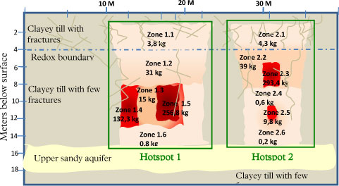
Figure 4.1 - Mass distribution at Vadsbyvej - vertical cross-section adapted from (Region Hovedstaden 2009)
The red zones on Figure 4.1 represent the residual phase, that is assumed to persist at the site. However in the model this residual phase cannot be taken into account. Furthermore the total mass given in the figure has to be converted to aqueous concentrations, in order to be used in the model.
The parameters used for such calculations are taken from (Region Hovedstaden 2008c)
- Clayey till porosity φ = 0.3
- Clayey till bulk density ρb = 1.96 kg/L
The aqueous concentrations are calculated with the following formula:
![]()
Where Cw is the aqueous concentration, Mtot is the total contaminant mass in the zone (without residual phase), Vtot is the total volume of the zone, φ is the porosity, ρb is the bulk density and Kd is the distribution coefficient. Some discussions are currently held concerning the sorption capacity of clay for chlorinated solvents [e.g. (Region Syddanmark 2007)]. Based on experiments conducted at DTU Environment with clay samples from Vadsbyvej and other Danish sites (DTU Environment 2008), the following distribution coefficients for the chlorinated solvents will be used:
- KdPCE = 1.4 L/kg
- KdTCE = 0.6 L/kg
- KdDCE = 0.12 L/kg
- KdVC = 0.04 L/kg
The simplified source distribution is shown on Figure 4.2. At hotspot 2 (zones A2 + B2), PCE is the dominant contaminant and it can be assumed that reductive dechlorination is not taking place. In contrast, hotspot 1 consists of PCE, TCE, DCE and VC in significant quantities, and the presence of daughter products is indicative of reductive dechlorination. This difference between the two hotspots will be taken into account for the modeling.
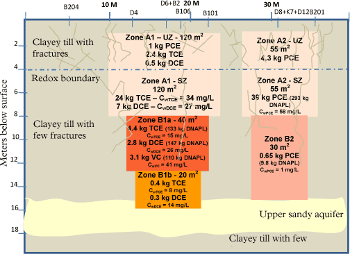
Figure 4.2 - Simplification of contaminant source distribution and average aqueous concentrations (disregarding the DNAPL phase)
4.2 Geological characterization – Fracture distribution
Intensive field experiments have been conducted at Vadsbyvej on fracture mapping from excavation, but data are available only for the upper 4 meters (above redox boundary). The model of this site is focusing on the zone below the redox boundary. From the field observations and some data extrapolation, a geological model is built for the clayey till, between 4 and 15 meters below surface. This model is based on a linear extrapolation of fracture frequency variation with depth observed at Vadsbyvej (red line on Figure 4.3). Therefore at 15 meters depth, a vertical fracture spacing of 5.6 meters is expected.
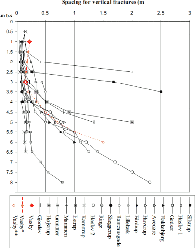
Figure 4.3 - Fracture distribution at 13 Danish clay till sites – in red Vadsbyvej (Christiansen and Wood 2006)
It can be assumed that the contaminant has migrated downward from the surface along the vertical fractures. Hence it is expected that the contaminant has spread into the matrix around the fractures. Therefore it is assumed that the two hotspots are each located symmetrically around two of the deepest vertical fractures. This configuration is shown in Figure 4.4.
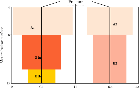
Figure 4.4 - Vertical fracture network and source location
4.3 Hydrogeological characterization
The hydraulic values (hydraulic conductivities and gradients) for clayey till and the underlying upper sandy aquifer are taken from (Region Hovedstaden 2008c) and summarized in Figure 4.5. These hydraulic conductivities are obtained from slug tests (one in the clayey till at 12 meters depth and two in the sand layer). The vertical hydraulic gradient was assumed based on head measurements in boreholes at different depth in the clay layer. The vertical hydraulic gradient and the bulk hydraulic conductivity correspond to a net recharge rate of 86 mm/year.
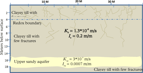
Figure 4.5 – Hydraulic characteristics for clayey till and upper sandy aquifer
A water balance can be performed on the source zone sketched on Figure 4.5. Assuming a source width of 22 meters, the water balance can be calculated per unit meter length (see Figure 4.6):
- Vertical water flow through the source zone
Qclay = KbivW = 1.8 m³ / year / m length - Horizontal water flow through the upper sandy aquifer
Qaq = KaqiaqTaq = 1.6 m³ / year / m length
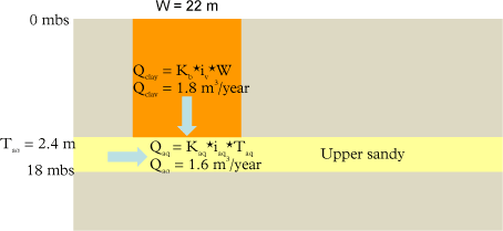
Figure 4.6 – Water balance for the upper sandy aquifer
Assuming that the hydraulic conductivity for the clay matrix is very low compared to Kb (generally in the order of 10-¹0 m/s (Jorgensen et al. 2002)), the average fracture aperture 2b is calculated from the bulk hydraulic conductivity and the spacing between two vertical fractures (2B = 5.6 m) to be 50 µm, with the following formula (Mckay et al. 1993):
![]()
Where ρ is the fluid density (kg/m³), g is the gravitational acceleration (m/s²) and μ is the viscosity (Pa.s).
4.4 Model configurations and scenarios
The model is used to assess the remediation time at Vadsbyvej using enhanced reductive dechlorination for different remediation scenarios, in comparison with the no remediation scenario. The remediation time can be evaluated with respect to the mass removal, the flux reduction and/or the concentration in the upper sandy aquifer. The results from the modeling will be compared with the remediation objectives described in Section 2.2.2.
The geometry (fracture distribution) presented in the previous sections is simplified; the present work focuses on downward transport from the till to the aquifer so horizontal features are neglected. For the same reason, only the fully penetrating vertical fractures are taken into account and an uniform fracture spacing is assumed (see Figure 4.7).
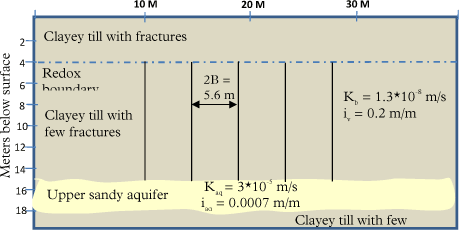
Figure 4.7 - Simplified geometry for Vadsbyvej
The two hotspots are modeled separately in order to reduce model size and computing time.
Different scenarios are considered for the modeling, in order to assess the effect of several remediation strategies compared to applying no remediation:
- Baseline = Reductive dechlorination occurs in hotspot 1, with a reduced amount of specific degraders (measured at the site) and no dechlorination occurs in hotspot 2.
- Remediation A = Reductive dechlorination occurs only at the injection depth.
- A1 - Reductive dechlorination is enhanced with injection of substrate and bacteria every meter
- A2 - Reductive dechlorination is enhanced with injection of substrate and bacteria every 25 cm
- Remediation B = Reductive dechlorination occurs in a 10 cm thick reaction zone around the injection depth (from the results at Rugårsdvej site)
- B1 - Reductive dechlorination is enhanced with injection of substrate and bacteria every meter
- B2 - Reductive dechlorination is enhanced with injection of substrate and bacteria every 25 cm
- Remediation C = Reductive dechlorination is enhanced with injection of substrate and bacteria every 10 cm, and dechlorination occurs in the whole matrix
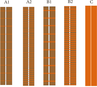
Figure 4.8 - Schema of remediation A1, A2, B1, B2 and C (from left to right) – the orange areas indicate the location where degradation occurs
4.5 Modeling results
In this section, we will focus on the modeling of hotspot 2, which is the one where reductive dechlorination does not occur naturally. It was decided to focus on this hotspot, as it is estimated that it will take longer to remediate.
4.5.1 Model parameters
Table 1 - Model parameters for Vadsbyvej
| Transport parameters | Value | Reference | |
| Fracture spacing 2B [m] | 5.6 | See Section 4.2 | |
| Fracture aperture 2b [µm] | 50 | See Section 4.3 | |
| Vertical hydraulic gradient Iv [m/m] | 0.2 | (Region Hovedstaden 2008c) | |
| Bulk hydraulic conductivity Kb [m/s] | 1.3*10-8 | ||
| Velocity in fracture vf [m/y] | 9478 | vf = KbI·2B/2b | |
| Matrix porosity φ | 0.3 | (Region Hovedstaden 2008c) | |
| Bulk density ρ [kg/L] | 1.96 | ||
| Tortuosity τ | 0.3 | τ = φ (Parker et al. 1994) | |
| Free diffusion coefficient D*i [m²/y] | (US EPA 2009) | ||
| PCE | 0.018 | ||
| TCE | 0.020 | ||
| DCE | 0.022 | ||
| VC | 0.026 | ||
| ETH | 0.033 | ||
| Sorption coefficient Kdi [L/kg] | See Section 4.1 | ||
| PCE | 1.4 | ||
| TCE | 0.6 | ||
| DCE | 0.12 | ||
| VC | 0.04 | ||
| ETH | 0 | ||
| Dispersivity in fracture [m] | 0.1 | assumed | |
| Microbial parameters | |||
| Maximum growth rate µi [1/d] | |||
| PCE | 3 | Assumed based on (Clapp et al. 2004,Lee et al. 2004) |
|
| TCE | 2 | (Miljøstyrelsen 2008a) | |
| DCE | 0.38 | ||
| VC | 0.14 | ||
| Specific yield Y [cell·µmol/L] | 5.2*108 | ||
| Biomass concentration X [cell/L] | |||
| Natural conditions (hotspot 1) | 107 | ||
| Enhanced dechlorination | 109 | from Gl. Kongevej (Region Hovedstaden 2008a) |
|
The velocity in the fracture can seem very high (9478 m/year), but such high values have been reported in the literature, with velocity up to 9125 m/year in (Mckay et al. 1993), 7800 m/year in (Sudicky and McLaren 1992), between 500-1000 m/year in (Harrar et al. 2007).
4.5.2 Hotspot 2
For hotspot 2, the results of the baseline and the different remediation scenarios are shown in term of both mass removal efficiency (Figure 4.9) and contaminant flux reduction (Figure 4.10).
The mass remaining in the system decreases very slowly for the baseline scenario and that less than half of the initial 40 kg is removed after 2000 years. Concerning the contaminant flux, it is expected to decrease with time from 80 to 25 g/year in 50 years. This simulated flux is higher compared to the measured flux at the site in the upper sandy aquifer (around 20 g/year from both hotspots). Several reasons could explain this difference:
- The initial concentrations in the source are overestimated
- The simulated fully penetrating fractures are not present at the hotspot
- Leaching from the source has occurred during the last 30 years, so the present flux could correspond to the simulated flux at 30 years (equal to 30 g/year)
- The bulk hydraulic conductivity (Kb) and/or the hydraulic vertical gradient (Iv) is overestimated
- The measured contaminant flux in the upper sandy aquifer is uncertain
Remediation scenarios A1 and A2, where dechlorination occurs at the injection depths only neither reduces the leaching time nor the flux compared to baseline scenario. This confirms the conclusions made in (Miljøstyrelsen 2008a); a reaction zone has to develop inside the matrix in order to be able to reduce clean-up times. This is also shown by the results for B1 and B2, where the mass is depleted in 200 and 50 years, respectively. However the contaminant flux for B2 is higher than for the baseline scenario during 7 years, due to the formation of more mobile daughter products (this phenomenon has been described in details in (Miljøstyrelsen 2008a).
As expected, remediation C is the most efficient with a mass depletion in 30 years, but again the contaminant flux peaks to 110 g/year and remains above the flux for the baseline scenario during 5 years. The composition of this flux can be seen in Figure 4.11, where the daughter products DCE and VC are dominant after few years.
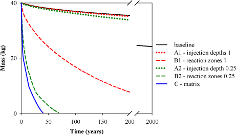
Figure 4.9 - Mass removal with time at hotspot 2. Note the break on the x-axis
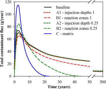
Figure 4.10 - Contaminant flux with time from hotspot 2. Note the break on the x-axis
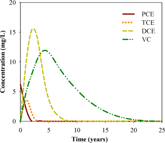
Figure 4.11 - Concentration at the fracture outlet for remediation scenario C (degradation in matrix)
For the defined remediation scenarios, it is assumed that reductive dechlorination occurs in the source for an infinite period after enhancement. However in most of the remediation plans the reductive dechlorination will be maintained (with regular injection of substrate) for only 10 years. Therefore remediation C is evaluated for the case where dechlorination stops 10 years after initiation (Figure 4.12). After dechlorination stops, the contaminant flux from source zone increases. This phenomenon is called “concentration rebound” (Mundle et al. 2007) and is due to the fact that one third of the initial mass is still present in the source zone. In Figure 4.12, it can also be observed that the rebound flux is higher than the flux resulting from the baseline situation (no remediation). This is due to the fact that after 10 years of enhanced dechlorination, the source zone consists of 50 % of DCE and VC, which are more mobile than the parent product PCE, and only 14% of the source was transformed to ethene.
This results show that dechlorination has to be maintained until most of the contaminated mass is converted to ethene, in order to avoid the risk of increasing the flux from the source zone and the contamination of the underlying aquifer, with very toxic daughter products (especially VC). This can be quantified by calculating the dechlorination degree in the source zone. After 10 years, the dechlorination degree is 60% only, which means that important quantities of contaminant have not been converted to ethene yet.
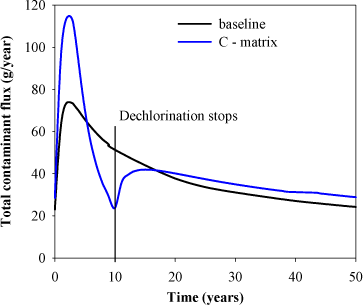
Figure 4.12 - Comparison of flux for baseline scenario and remediation C (where dechlorination stops after 10 years)
4.5.3 Hotspot 1
Given the results for hotspot 2, only the scenarios baseline, B2 and C are simulated for hotspot 1. For the baseline scenario, dechlorination is assumed to occur with degradation rates reduced by a factor 100 (compared to enhanced dechlorination). The results are given in Figure 4.13 and Figure 4.14.
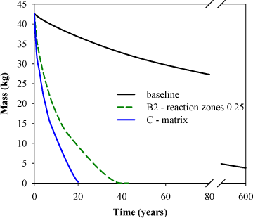
Figure 4.13 - Mass removal with time at hotspot 1. Note the break on the x-axis
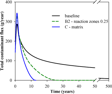
Figure 4.14 - Contaminant flux with time from hotspot 1. Note the break on the x-axis
The same trend is observed for hotspot 1, but the mass removal is faster than for hotspot 2. This is due to the natural degradation occurring at the source and the fact that the source consists mainly in daughter products TCE, DCE and VC, which are more mobile than PCE. The composition of the source also explains the higher contaminant flux that is simulated for the baseline scenario, although the same mass is present in the system at the initial time (around 40 kg).
4.5.4 Concentration in underlying sandy aquifer
The major concern in the underlying sandy aquifer is the concentration of vinyl chloride, therefore only this compound is used in the model. The model for the underlying aquifer developed in (Miljøstyrelsen 2008a) is used to simulate the plume development of VC for three different scenarios (baseline, B2 and C). The resulting VC flux from hotspots 1 and 2 is used as a contamination source for the aquifer (see Figure 4.15).
The parameters used for the aquifer are summarized in Table 2. It is important to notice that no degradation is assumed to occur in the aquifer. The flow factor (ff), defined as the ratio of the recharge rate and the mean specific discharge is very high (12%). This shows a significant recharge locally, however the recharge is most probably to high at a larger scale. Otherwise we will need very high flow velocities (high Kaq and iaq) in the upper sandy aquifer in order to get a reliable water balance. This can be explained by different reasons:
- The bulk hydraulic conductivity (Kb) and/or the vertical hydraulic gradient throughout the clay till (Iv) is much lower outside the source zone.
- An intermediate sand layer in the clayey till causes horizontal transport
- There is a hydraulic connection between the upper sandy aquifer and the regional chalk aquifer, and the downward water flow to this chalk aquifer is not negligible.
Table 2 - Parameters for the upper sandy aquifer
| Parameters | Symbol | Value | Unit | Reference |
| Aquifer thickness | Taquifer | 2.4 | m | (Region Hovedstaden 2007) |
| Hydraulic conductivity | Kaq | 3*10-5 | m/s | |
| Horizontal hydraulic gradient | Iaq | 0.0007 | - | |
| Effective porosity | φaq | 0.2 | - | |
| Recharge rate | R | 82 | mm/year | R = Kb*Iv |
| Flow factor | ff | 12 | % | ff = R/(Kaq*Iaq) (Miljøstyrelsen 2008a) |
| Longitudinal dispersvity | αL | 0.1 | m | (Hojberg et al. 2005) |
| Vertical transverse dispersvity | αT | 0.005 | m | |
| Source width | W | 22 | m | See Figure 4.4 |
As noted in (Miljøstyrelsen 2008a), the groundwater velocity in this aquifer is very low (around 3m/year), therefore a transient model is used in this part.
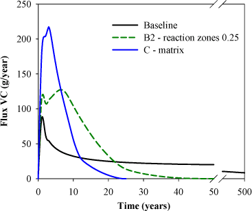
Figure 4.15 - VC flux from hotspots 1 and 2 for three different scenarios. Note the break on the x-axis
The resulting vinyl chloride concentration in the aquifer, just downstream of the source, is shown in Figure 4.16, where it can be seen that enhanced reductive dechlorination in the clay tends to increase the VC concentration in the aquifer, compared to the baseline scenario. This result was expected from the contaminant flux from the source, where it was seen that the formation of daughter products during reductive dechlorination entails an increase in VC flux from the source zone into the aquifer. However these high concentrations decrease after 30-40 years, compared to the baseline case, where the concentration is expected to maintain a value around 1000 µg/L during more than 100 years. The time lag between the peak in the flux from the source and the peak of concentration in the aquifer is due to the very slow groundwater velocity (3m/year, that can be compared with the assumed width of the source W = 22 meters).
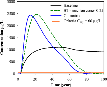
Figure 4.16 – Average VC concentration in upper sandy aquifer, under the source zone. Orange line = remediation criteria for the aquifer (CVC = 60 µg/L)
4.5.5 Comparison with field data
ERD has not yet been applied to Vadsbyvej, so it is not possible to compare the modeling results with some field data. However extensive field investigations have been performed at the site to characterize the source zone, the two hotspots, and the contaminant plume in the underlying sandy aquifer. These data can give a qualitative comparison with the modeling approach used in the present study.
The concentration in the sandy aquifer is monitored with several boreholes, shown in Figure 4.17. The relative contaminant composition based on the concentrations for the different boreholes (see Figure 4.18) shows that the daughter products DCE, VC and ethene are dominant in the sandy aquifer. This is very different from the source composition (see Figure 4.2), where TCE/DCE are dominant in hotspot 1 and PCE is dominant in hotspot 2. As the natural dechlorination in the sandy aquifer is expected to be negligible (Region Hovedstaden 2007), the domination of daughter products in the sandy aquifer can be explained by a faster breakthrough of these more mobile compounds. This phenomenon is predicted by the model and the results from Vadsbyvej tend to qualitatively support the findings from numerical modeling.
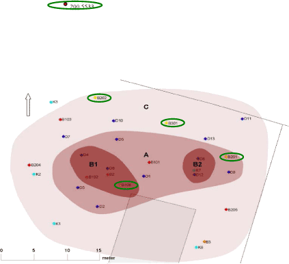
Figure 4.17 – Situation plan with the two hotspots (B1 and B2), and the boreholes monitored in the sandy aquifer (green circles)
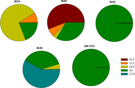
Figure 4.18 - Contaminant distribution based on concentration in the sandy aquifer for 5 boreholes
4.5.6 Comparison with remediation objectives
The functional remediation criteria defined for Vadsbyvej have been presented and explained in Section 2.2.2:
- a stationary or decreasing contaminant flux to the upper sandy aquifer compared to the baseline of 10 g/year (sum of chlorinated solvents)
- a stationary or decreasing concentration of vinyl chloride in the upper sandy aquifer compared to the baseline of 60 µg/l.
4.5.6.1 Remediation criterion on the contaminant flux
The contaminated flux criterion out of the clay can be compared with the results from Sections 4.5.2 and 4.5.3 (Figure 4.10 and Figure 4.14), where the contaminant flux from the source zone was assessed for different scenarios. From the different simulations, it results that this criterion will be reach after:
- 700 years for the baseline scenario
- 30 years for remediation B2
- 15 years for remediation C
For remediation B2 and C, these timeframes are defined by the flux reduction occurring at hotspot 2 only, as the flux from hotspot 1 reduces much faster.
However these timeframes are valid only if dechlorination goes on in the system, as it has been seen in Section 4.5.2 that there is a risk of rebound of contaminant after dechlorination stops. This means that reaching a contaminant flux below 10 g/year does not necessarily means that the flux will remain below this value when dechlorination stops. It was found that dechlorination has to be maintained during 25 years at hotspot 2 (remediation C), in order to ensure a contaminant flux below the remediation criteria several years after dechlorination stops. This is illustrated in Figure 4.19. This period increases to 40 years in case of remediation B2.
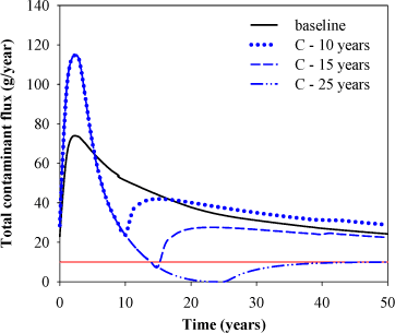
Figure 4.19 - Total contaminant flux from hotspot 2 for remediation C (matrix) for different termination times (10, 15 and 25 years). In red the actual remediation objective (10 g/year)
In practice it is very difficult to measure a contaminant flux at a field site, therefore it is interesting to evaluate the average water and total concentration that needs to be reached at hotspot 2 to ensure the respect of the remediation criteria.
For remediation C, this corresponds after 25 years of dechlorination to an average aqueous concentration of the chlorinated compounds in hotspot 2 below 20 mg/L, which corresponds to an average total concentration of 4 mg/kg. The initial average total concentration in hotspot 2 is 34 mg/kg, so this concentration has to be reduced by a factor of 10. The corresponding concentrations in case of remediation B2 are in the same range.
Furthermore it has been seen that in order to prevent rebound after remediation stops, an important part of the source has to be converted to ethene. This can be ensured by defining a remediation criterion on the dechlorination degree that has to be reached in the source zone. The model result shows that a dechlorination degree of 90% has to be achieved in the source zone, in order to prevent rebound.
4.5.6.2 Remediation criterion on VC concentration in the underlying aquifer
This criterion can be compared with the results from Sections 4.5.4 (Figure 4.16), where VC concentration in the underlying sandy aquifer was assessed for different scenarios. From the different simulations, it results that this criterion will be reached after:
- More than 700 years for the baseline scenario
- 80 years for remediation B2
- 70 years for remediation C
These long timeframes, compared to the ones for flux criteria, are due to the very slow velocity in the sandy aquifer (3m/year), and illustrates that in case of remediation, a buffer zone has to be created in the aquifer in order to enhance anaerobic dechlorination.
In a steady-state scenario, the concentration of contaminant downstream the source is reduced by 30% compared to the concentration at the bottom of the source. Therefore a VC concentration of 60 µg/L in the aquifer, corresponds to a VC concentration of 90 µg/L at the fracture outlet, which corresponds to a flux of vinyl chloride of 3.5 g/year (which is very close to the remediation criterion on flux). We can then see that the remediation criteria on flux and on concentration are closely linked together, and have been wisely chosen in the present case.
4.6 Sensitivity analysis on parameters
The most sensitive parameters identified in (Miljøstyrelsen 2008a) are varied within a realistic range of uncertainty in order to assess the influence on the results for the baseline and remediation C scenarios. The chosen parameters can be seen in Table 3. For some parameters (foc and φ), the initial aqueous concentration was modified to maintain the same initial mass (according to Equation ). For Kb and 2B, the value of the fracture aperture 2b is also modified to ensure a correct water balance. The last parameter is the reaction rate, which depends on the maximum growth rate µi, the biomass concentration X and the specific yield Y.
Table 3 - Parameters and range for uncertainty analysis
| Parameter | Baseline value | Min value | Max value |
| Bulk hydraulic conductivity Kb | 1.3*10-8 m/s | 10-9 m/s | 10-7 m/s |
| Fraction of organic carbon foc | 1 % | 0.1 % | 2 % |
| Fracture spacing 2B | 5.6 m | 2 m | 8 m |
| Porosity φ | 30 % | 20 % | 40 % |
| Reaction rate µiX/Y | Διϖιδεδ βψ 10 (/10) | Multiplied by 10 (*10) |
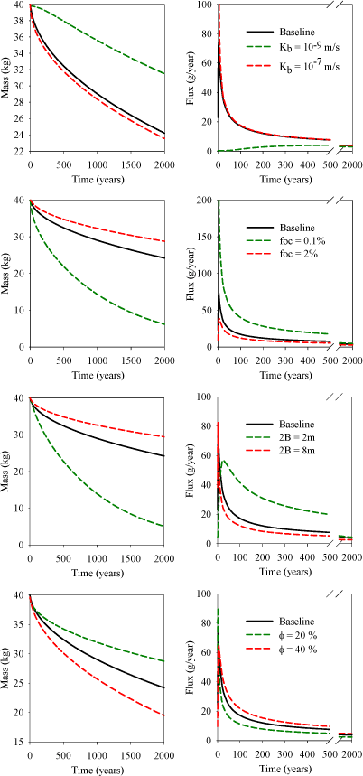
Figure 4.20 - Uncertainty analysis for baseline scenario at hotspot 2. Note the different scales on y-axis and the break on x-axis.
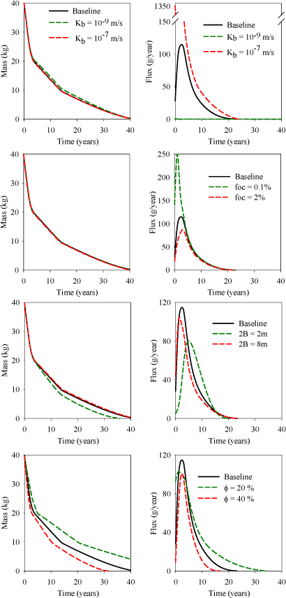
Figure 4.21 - Uncertainty analysis for remediation C scenario at hotspot 2. Note the different scales on y-axis and the break on x-axis.
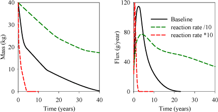
Figure 4.22 - Uncertainty of reaction rates on remediation C at hotspot 2
4.6.1 Sensitivity analysis for the baseline scenario
For the baseline scenario (no dechlorination), the system is mainly controlled by diffusion processes in the matrix with a high sensitivity to fracture spacing (2B), sorption coefficient (foc) and porosity (φ). This last parameter controls the effective diffusion coefficient in the matrix. The system is also very sensitive to the bulk hydraulic conductivity (Kb), which controls the quantity of clean water entering the fracture and flushing the contaminant. This last parameter influences both the mass removal and the contaminant flux, which varies by one order of magnitude, with variations in Kb. As explained in (Miljøstyrelsen 2008a), the limiting process is the back diffusion from the matrix into the fracture. The high sensitivity to the transport processes mean that site specific characterization is needed for the key parameters such as fracture spacing, sorption coefficients, porosity of the matrix and water balance of the clay unit.
4.6.2 Sensitivity analysis for remediation C (degradation in the whole system)
The results for remediation C are more sensitive to the microbial parameters (the reaction rate). When dechlorination occurs in the whole matrix, the system is controlled by the kinetics of the reactions. For this system, the clean-up time is mainly affected by the reaction rate µiX/Y. By increasing the reaction rates by one order of magnitude, the clean-up time is divided by 10, from 28 to 3 years. Conversely, a decrease by one order of magnitude of these reaction rates will multiply the clean-up time by 7 (to 180 years). The biomass concentration can easily vary by one order of magnitude from site to site, therefore the high sensitivity of the results of remediation C to this parameter highlights the need for a site specific characterization of the biomass populations, and for a better understanding of the microbial processes during reductive dechlorination.
In term of mass removal, the results are not sensitive to the other parameters (Kb, foc, and 2B), besides porosity (φ). However the flux magnitude varies significantly and this can have an influence on the contamination of the underlying aquifer during and after remediation treatment.
Version 1.0 July 2009, © Danish Environmental Protection Agency