Guidelines on remediation of contaminated sites
Appendix
5.8
Standard data to be used for risk assessments of groundwater
A series of calculation parameters must be used in connection with risk assessments of groundwater. This appendix provides examples of standard data which can be used in these calculations.
It must be stressed that more conservative values must be used if the parameters used are estimates, regional rather than local, or uncertain for other reasons. If risk assessment is to be precise and conservative estimates are to be avoided, more calculation data must be site-specific.
1 Groundwater recharge
Calculations of the amount of infiltrating soil water at a contaminated site include assessments of groundwater recharge proportion of precipitation.
In certain local areas, counties have knowledge of the proportion of precipitation which comprises groundwater recharge. However, for most areas it is necessary to use net precipitation as a conservative alternative. Figure 1 outlines the average net precipitation in Denmark and its distribution among areas /1/.
Evaporation from soil and plants (actual evaporation) is included in calculations of net precipitation and is established by means of model calculations by the computer model EVACROP. Evaporation varies with crop type/vegetation type and soil type. In these calculations, crops are estimated to comprise a mixture of 50% winter crops and 50% summer crops, a mixture which will cover 60-70% of the agricultural areas. The estimated soil type for Jutland is a mixture of coarse and fine grain soil, and the soil type for the rest of Denmark is set to be clay soil mixed with sand. These assumptions result in an actual evaporation of 400 mm per year for Jutland and 440 mm per year for the rest of Denmark. Local deviations from these typical values will occur due to land use and crop distribution. As net precipitation is the difference between precipitation and actual evaporation, this will occasion deviations from the values shown in Figure 1; for this reason, these values will have certain imperfections.

Figure 1
Net precipitation in Denmark (mm), mean 1961-90; /1/.
Deviations from the values shown here of up to approximately 40 mm per year are estimated to be common, but deviations of more than 60 mm will be rare.
2 Hydraulic conductivity and effective porosity
The hydraulic conductivity k is highly variable, and for this reason should always be determined at the specific site. Table 1 states typical values for horizontal hydraulic conductivity and effective porosity for various soil types /2, 5/.
In addition to this, certain known values for vertical permeability in clayey till are given /3,4/.
Table 1
Typical values for hydraulic conductivity (m/second) for various soil types /2,3,4/
and effective porosity /5/.
Material |
Hydraulic conductivity, k (m/s) |
Effective porosity, eeff. |
Horizontally: Clay soil (near the surface) Deep clay strata Silt Sand, fine Sand, medium grain Sand, coarse Gravel Organic silt Sandstone Limestone Rock, fissured and weathered |
10-8 - 10-6 10-8 - 10-2 10-5 - 5 x 10⁻⁵ 10-5 - 5 x 10⁻⁵ 5 x 10⁻⁵ - 10-4 2 x 10⁻⁴ - 10-3 10-3 - 10-2 ~ 10-10 - 10-8 - 10-5 10-7 - 10-5 10-8 - 10-4 |
0.01-0.2 0.01-0.2 0.01-0.3 0.1-0.3
0.15-0.3 0.2-0.35 0.1-0.35
0.1-0.4 0.01-0.24 |
Vertically: Clay till Clayey till Clayey till |
|
|
3 Hydraulic gradient
The hydraulic gradient, i, is not a standard parameter. The hydraulic gradient must be determined locally on the basis of water level measurements in investigation wells. Alternatively, the hydraulic gradient can be determined on the basis of local maps of the potentiometric surface.
4 Dispersivities
For risk assessments of groundwater, the longitudinal dispersivity aL, cf. Section 5.4 and Appendix 5.6 of these guidelines, is used for calculating mixing thickness in the saturated zone (steps 2 and 3 of step-by-step risk assessment).
Figure 2 shows known values for the longitudinal dispersion as a function of distance. The size of the symbols indicate the reliability of the tests /2,6/.
Calculations of the mixing thickness dm show that mixing thickness increases with dispersivity. The greater the longitudinal dispersivity, the greater the mixing thickness. For this reason, low values must be selected for aL to ensure conservation calculations. Figure 2 shows the longitudinal dispersivity for a given distance on the solid curve.
5 Retardation factors
For sorbing substances, soil-water velocity Vp can in some formulae be replaced by the spreading velocity of the substance front Vs. The correlation between these factors can be described as (cf. Appendix 5.6):
VS = VP/R, where R is the retardation factor.
The retardation factor R is not a standard parameter, where a value applies to a larger geographic area.
The retardation factor depends on the substances involved, and on the bulk density of soil r b, actual soil contents of organic substances foc, and on the octanol-water distribution coefficient Kow. The content of organic substances foc for various soil types is found in Appendix 5.3, Table 1, and log Kow values for various substances can be found in Appendix 5.5, Tables 1-5.
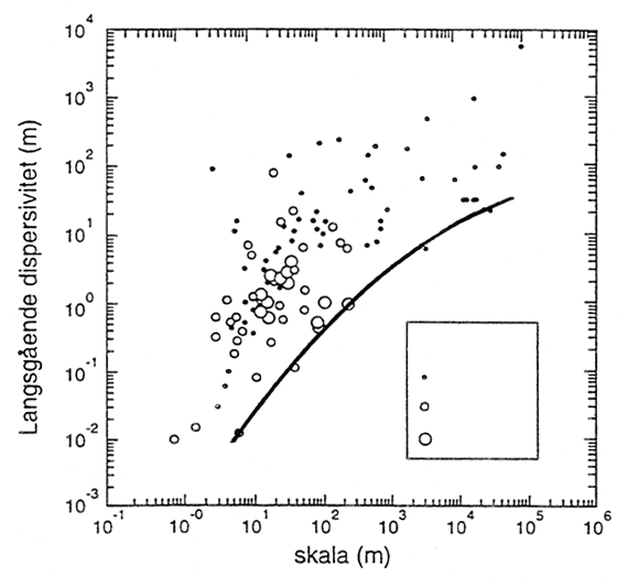
Figure 2
Longitudinal dispersivity as a function of distance /2,6/. The sizes of the symbols indicate the reliability of the
tests. For calculations of mixing thickness in saturated zones, aL-values from the solid curve are used.
Given the assumptions that log Kow < 5 and foc > 0.1%, the distribution coefficient Kd can be calculated by means of Abdul’s formula /1/:
log Kd = 1.04 × log Kow + log foc – 0.84
The retardation factor can then be calculated by means of the formula:
R = 1 + rb/ew × kd
where
rb is the soil density [ML-3],
ew is soil porosity when saturated with water [unitless],
and Kd is the distribution coefficient.
Examples of calculations of retardation factors are found in Appendix 5.7.
6 1st Order degradation constants
As was outlined in Appendix 5.6, the relative substance concentration C on the basis of a 1st order degradation can be calculated as:
C3 = C2 × exp (-k1 × t)
| where | t | is the time period, during which degradation occurs [T], |
| C3 | is the resultant contamination concentration of the most contaminated zone of the groundwater aquifer after having taken degradation into account [ML-3], | |
| C2 | is substance concentration before degradation[ML-3], | |
| k1 | is the relevant 1st Order degradation constant [T-1]. |
The degradation constants are substance specific, and moreover highly dependant on
geological and hydrogeological conditions. For example, the degradation constants are
often highly dependant on redox conditions. For many contaminants, degradation occurs
fastest under aerobic conditions, other contaminants are exclusively degraded under
anaerobic conditions, and some contaminants exclusively degrade under methanogenic
conditions.
As yet, only very few examples of degradation constants determined in field conditions are available.
The degradation constants established so far vary greatly from one another. For this reason, it would be most favourable to determine the degradation constant at each site. Alternatively, conservative degradation constants must be used in calculations.
If calculations are made for degradation, it is important to ensure that there is potential for degradation throughout the entire period for the entire geographical area used in the calculations. For instance, in cases of aerobic degradation it must be ensured that oxygen is present throughout the entire period and the entire geographical degradation area. This is ensured by means of monitoring.
As part of a technology project, the Environmental Protection Agency has compiled 1st order degradation constants which are deemed representative of Danish conditions /7/. Table 2 shows a compilation of these degradation constants.
Table 2
1st order degradation constants /5/;
compiled after Kjærgaard et al /7/.
Contaminant |
1st order degradation constant (day-1) |
Comment |
|
|
Aerobic |
Anaerobic |
|
BTEXs Benzene |
|
|
|
0.01-0.2 |
0.001-0.003 |
Unlikely to be degradable in denitrified conditions |
|
Toluene |
0.05-0.2 |
0.01-0.1 |
|
Ethylbenzene |
0.01-0.1 |
0.002-0.03 |
Educated guess at aerobic degradation due to insufficient data |
o-xylene |
0.02-0.1 |
0.002-0.02 |
|
m/p-xylene |
0.001-0.02 |
0.002-0.03 |
|
Chlorinated solvents |
|
|
|
1,2-dichloroethane |
0 |
0.001-0.007 |
|
1,2-dichloroethene |
0 |
0.001-0.009 |
|
cis-1,2-dichloroethene |
0 |
0.0001-0.002 |
|
Dichloromethane |
0 |
0.0001-0.06 |
|
Tetrachloroethylene |
0 |
0.0005-0.004 |
|
1,1,1-trichloroethane |
0.005-0.006 |
0.0005-0.005 |
|
Trichloroethylene |
0 |
0.0001-0.008 |
|
Trichloromethane |
0 |
0.006-0.1 |
|
Chloroethylene (Vinylchloride) |
0.01* |
0.0004-0.002 |
*Conservative estimate based on a single investigation |
Other substances |
|
|
|
Phenol |
0.07-0.4 |
0.001* |
*Conservative estimate based on a single investigation |
References
| /1/ | Mikkelsen, H. 1993. Nettonedbør. Udkast. (‘Net
Precipitation. Draft’) Statens Planteavlsforsøg. [Tilbage] |
| /2/ | Kemiske stoffers opførsel i soil og grundwater
(‘Chemical Substance Behaviour in Soil and Groundwater’) Projekt om soil og
grundwater (‘Project on Soil and Groundwater’), No. 20. The Environmental
Protection Agency, 1996. [Tilbage] |
| /3/ | Jørgensen, P. R. (Danish Geotechnical Institute) and Spliid,
N. H. (National Environmental Research Institute): Migration and Biodegradation of
Pesticides in fractured Clayed Till. [Tilbage] |
| /4/ | Grundvandsstrømning og udvaskning af forurening i
moræneler. Geoteknisk Institut informerer. (‘Groundwater Percolation and
Contamination Wash-out in Clayey till. Information from the Danish Geotechnical
Institute’) GI Info 5.8, 1993. [Tilbage] |
| /5/ | Wiedemeier, T.H. et al. 1996. Technical protocol for
evaulating natural attenuation of chlorinated solvents in groundwater. Draft –
Revision 1. Air Force Centre for Environmental Excellence, Technology Transfer Division,
Brooks Air Force Base, San Antonio, Texas. [Tilbage] |
| /6/ | Gethar, L. W., Welty C. and Rehfeldt K. R. 1992:A critical
review of data on field-scale dispersion in aquifers. Water Resources Research, 28,
1955-1974. [Tilbage] |
| /7/ | Kjærgaard, M., Ringsted, J.P., Albrechtsen, H.J. og Bjerg,
P.L. Naturlig nedbrydning af miljøfremmede stoffer i soil og grundwater
(‘Natural Degradation of Alien Substances in Soil and Groundwater’) the Danish
Geotechnical Institute in collaboration with the Technical University of Denmark. A
technology development project for the Environmental Protection Agency, 1998. [Tilbage] |