| Front page | | Contents | | Previous | | Next |

The indoor and outdoor concentrations of particulate air-pollution and PAHs in different size fractions and assessment of exposure and health impacts in the Copenhagen population

3 PM in indoor and outdoor air

• 3.1 PM1, PM2.5 and PMinh
• 3.1.1 Intrasite relationships and prediction of missing PM data
• 3.1.2 Outdoor-outdoor relationships and prediction of missing data
• 3.1.3 The contribution from traffic to the particulate air-pollution
• 3.1.4 Indoor-outdoor relationships
• 3.2 Seasonal variation and comparison with PM guidelines
• 3.2.1 Seasonal variation
• 3.2.2 Comparison with air-pollution guidelines
• 3.3 Evaluation of particle induced health effects
• 3.3.1 Assessment of adverse health effects related to PM2.5
• 3.3.2 Increase per million per 10 g/m3 increase in PM2.5
• 3.3.3 Health effect assessment based on the PM2.5 distribution function

In this chapter we discuss the levels of particulate air-pollution indoors and outdoors at Jagtvej and in the urban background. The relationships between PM₁, PM_2.5 and PM_inh were investigated at the three measuring points to create a regression line model for estimating missing data. Statistical analyses were conducted to suggest a yearly average concentration of the three PM fractions. Linear regression analysis are performed to investigate the contribution for all three size fractions in the urban background on the particulate air-pollution in the street as well as the influence from both Jagtvej and urban background to the particulate air-pollution indoors in the apartment studied.

3.1 PM₁, PM_2.5 and PM_inh

Tables 3.1-3.3 list the weekly measured and estimated air-pollution mass concentrations indoors (IN) and outdoors (EXT) at Jagtvej and in the urban background air (NIOH). The tables include PM₁ 2001 fall data from Sharma (2002) and predicted mass-concentrations for weeks with missing data (see section 3.1.1).

Table 3.1: Weekly indoor mass-concentration at Jagtvej

§ Measured PM₁ data from Sharma (2002).

$ Ventilation slits moved from the living room window to the bedroom window facing the backyard.

£ The artificial door to the sealed off kitchen was open the last 24 h.

Shaded cells: modelled data based on linear regression analysis

eq. # in shaded cells refers to which regression equation in section 3.1.1. that was used.

Tabel 3.2: Weekly street canyon mass-concentrations at Jagtvej

§ Measured PM₁ data from Sharma (2002).

Shaded cells: modelled data based on linear regression analysis

eq. # in shaded cells refers to which regression equation in section 3.1.1. that was used.

Tabel 3.3: Weekly urban background mass-concentrations at NIOH

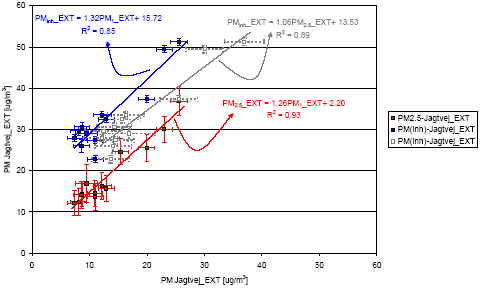
§ Data modelled based on data in Sharma (2002).

Shaded cells: modelled data based on linear regression analysis

eq. # in shaded cells refers to which regression equation in section 3.1.1. that was used.

The results show a wide range in the weekly particulate air-pollution at all sites. High levels occur during January 9 – 23 and March 27 – April 24, 2002 with PM₁, PM_2.5 and PM_inh reaching up to 26.00±1.56, 36.92±3.45 and 58±(95% CI) g/m³ at Jagtvej, respectively (Tables 3.1-3.3; Fig. 3.1.1a). Lower air-pollution concentrations were observed at the NIOH with measured concentrations reaching 23.30±1.38 g/m³ and 39.27±1.05 g/m³ for PM₁ and PM_inh, respectively. The lowest air-pollution level was observed February 6 – 13 with a PM₁ concentration of 7.40±1.32 g/m³ and 4.05±1.84 g/m³ at Jagtvej and NIOH, respectively.

Independent of measuring site, PM₁ on average makes appr. 70 wt% of PM_2.5. The average content of PM_2.5 in inhalable dust was 54 and 69 wt% at Jagtvej_EXT and NIOH, respectively. In the uninhabited apartment PM_inh consisted almost entirely of PM_2.5.

3.1.1 Intrasite relationships and prediction of missing PM data

Scatter plots show that there generally is a strong correlation between the PM₁, PM_2.5 and PM_inh from the same measuring locality. Fig. 3.1 shows an example of this co-variation for the PM measurements at Jagtvej_EXT.

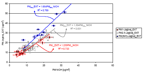
Figure 3.1: Scatter plot showing the high correlation for PM_2.5 vs. PM₁ (R²=0.93), PM_inh vs. PM₁ (R²=0.85) and PM_inh vs. PM_2.5 (R²=0.89) between the individual PM size fractions at Jagtvej_EXT.

The strong relationship between the fine and coarse size-fractions may be caused by the fact that the bulk of the particulate air-pollution is dominated by PM₁. Another explanation may be that the dominant particle sources emit particles in both fine and coarse particles. Regression analysis showed that the relationships between the size fractions measured at the same site enable prediction of missing PM-concentration data with p-values of at least 0.035:

1) PM_2.5_IN = 4.66 + 0.952 · PM₁_IN (p=0.000; R²=77.3%)

2) PM_inh_IN = 5.12 + 0.801 · PM₁_IN (p=0.003; R²=83.7%)

3) PM_inh_IN= 3.16 + 0.783 · PM_2.5_IN (p=0.003; R²=65.4%)

4) PM_2.5_EXT = 2.19 + 1.26 · PM₁_EXT (p=0.000; R²=93.5%)

5) PM_inh_EXT = 15.7 + 1.32 · PM₁_EXT (p=0.000; R²=84.7%)

6) PM_inh_EXT = 13.5 + 1.06 · PM_2.5_EXT (p=0.000; R²=88.6%)

7) PM_2.5_NIOH = 5.44 + 0.859 · PM₁_NIOH (p=0.003; R²=76.7%)

8) PM_inh_NIOH = 12.9 + 0.818 · PM₁_NIOH (p=0.035; R²=44.7%)

9) PM_inh_NIOH = 3.14 + 1.23 · PM_2.5_NIOH (p=0.012; R²=62.1%)

The regression equation for prediction of PM_inh_NIOH from PM₁_NIOH had a relatively poor, but still significant p-value (p=0.035). The probability was slightly improved (p=0.012) using the PM_2.5 data, but R² values were relatively low for all analysis intrasite NIOH regressions. Much better statistics were obtained using the regression equations between the data from JGTVJ_EXT and NIOH (see below). Consequently equations a to f were used to predict missing values at JGTVJ_IN and JGTVJ_EXT in Tables 3.1 and 3.2, respectively.

3.1.2 Outdoor-outdoor relationships and prediction of missing data

Similar to the intrasite co-variation, regression analysis showed a strong relationship between the levels of particulate air-pollution in the Jagtvej street canyon (Jagtvej_EXT) and the PM levels in the urban background at NIOH (Fig. 3.2):

10) PM₁_NIOH = - 3.50 + 0.998PM₁_EXT (p=0.000; R²=90.1%)

11) PM_2.5_NIOH = 1.93 + 0.914PM₁_EXT (p=0.000; R²=83.1%)

12) PM_2.5_NIOH = - 0.36 + 0.773PM_2.5_ EXT (p=0.000; R²=86.0%)

13) PM_inh_NIOH = - 2.82 + 0.667PM_inh_EXT (p=0.000; R²=85.5%)

14) PM₁_EXT = 4.48 + 0.903PM₁_NIOH (p=0.000; R²=90.1%)

15) PM_2.5_EXT = 2.85 + 1.112PM_2.5_NIOH (p=0.000; R²=86.0%)

16) PM_inh_EXT = 8.56 + 1.281PM_inh_NIOH (p=0.000; R²=85.5%)

Owing to better statistics than observed for intrasite regression statistics (equations 7 to 9), the equations numbered 10 to 16 were used to generate PM concentrations for the missing data at NIOH and Jagtvej_EXT (Table 3.3) when applicable.

Figure 3.1.2.1 shows a scatter plot with both measured and predicted PM data and associated linear regression equations. It is evident that the estimated values for the missing data generally fit very well with the trend of the measured data. Hence, the estimated data were included in the further data analysis presented hereafter.

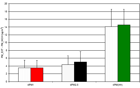
Figure 3.2: Scatter plot showing the correlation between PM in the Jagtvej street canyon and PM in the urban background at NIOH. The plot includes both measured and predicted data from the 2002 campaign.

3.1.3 The contribution from traffic to the particulate air-pollution

Based on the ultrafine to fine particle size of car exhaust, one may expect that traffic mainly would contribute significantly to the concentration of PM₁ and have less pronounced effects on PM_2.5 and PM_inh. However, coarse particles such as suspended dust as well as tire and brake wear particles also play an important role. Previous analysis by ) has shown that the contribution from "traffic" to PM₁₀ was on the order of 11.4 g/m³. In fact chemical analysis and particle characterization suggest that fine to coarse brake wear particles are quite significant constituents of this size fraction in the streets in Copenhagen (pers. comm. P. Wåhlin, NERI;.

The current study can provide an assessment of the contribution from traffic to both PM₁, PM_2.5 and PM_inh, assuming that the traffic contribution (dPM) can be estimated from the equation:

17) dPM = PM_EXT – PM_NIOH

Including estimated PM concentrations, equation 17 suggests that traffic on average contributes with 3.5±1.9 μg/m³ PM₁; 5.0±2.7 μg/m³ PM_2.5 and 14.6±4.0 μg/m³ PM_inh, respectively at Jagtvej (Fig. 3.3). Omitting estimated PM concentrations, did not change the amount of traffic dPM emissions significantly (Fig. 3.3). Noteworthy, the estimate of dPM_inh (14.6±4.0 μg/m³) is within the same range as determined for PM₁₀ (11.4 μg/m³) by Palmgren et al. (2002). Despite PM₁₀ and PM_inh are not directly comparable measures the results support each other. However, the estimates of dPM from this calculation should still be considered minimum values, because resuspension of dust and especially traffic emissions also contribute to the PM concentrations in the urban background.

Figure 3.3: Average contribution from traffic (dPM) to the particulate air-pollution at Jagtvej estimated from equation 17. Filled bars are PM contribution from traffic based on both modeled and measured data, whereas dotted bars are estimates based on measured data alone. Note there is only a minor difference between the estimates based on measured data alone and estimates including modeled data.

3.1.4 Indoor-outdoor relationships

Indoor-outdoor (I/O) mass-concentration ratios is often used to assess the penetration of outdoor air into the indoor environment. However, I/O-ratios, of-course cannot tell the origin of the particulate air-pollution. Because the measurements were conducted in an uninhabited apartment, the influence from indoor sources was reduced to a minimum in this study. Hence, the indoor PM concentrations should be a good measure of particles that have penetrated from the outdoor environment. Further assessment of the particle infiltration from outdoors is made by statistical analysis of the relationships between the indoor and outdoor air-pollution levels.

3.1.4.1 I/O ratios

Table 3.4 lists the I/O (indoor/outdoor) ratios for the particulate air-pollution in the apartment compared to the air-pollution levels in the Jagtvej street canyon and in the urban background (NIOH). Table 3.4 also lists the measured average total air-exchange rates in the apartment.

The average I/O-ratios for PM₁ (0.770.21) and PM_2.5 (0.770.24) were almost the same using the outdoor PM concentrations from Jagtvej. The average I/O-ratio was notably higher: 1.120.34 and 1.050.35 for PM₁, and PM_2.5, respectively when indoor concentrations were compared to the city background data from NIOH. The I/O-ratio for PM_inh was lower than observed for PM₁ and PM_2.5, averaging 0.390.10 and 0.480.17 using street and urban background data, respectively. This was expected due to the poorer penetration efficiency for coarse particles.

It is important to note that the average PM₁ and PM_2.5 I/O ratios were higher than or close to unity when the I/O-ratios was calculated based on urban background data. This may be of relevance for epidemiological studies that normally use urban background concentrations as a reference for estimating the frequency of adverse health effects. Since, the average I/O-ratios for PM₁ and PM_2.5 exceed unity, when calculated based on urban background PM concentrations and not when calculated based on street concentrations, the street PM appears to have significant influence on the indoor particle concentration in this fourth floor apartment. From the total mass concentrations, the bulk, however, appears still to be controlled by the urban background concentrations.

Table 3.4: I/O-ratios for indoor PM₁, PM_2.5 and PM_inh versus the particulate air-pollution in the Jagtvej street canyon (IN/EXT) and in the urban background (IN/NIOH).

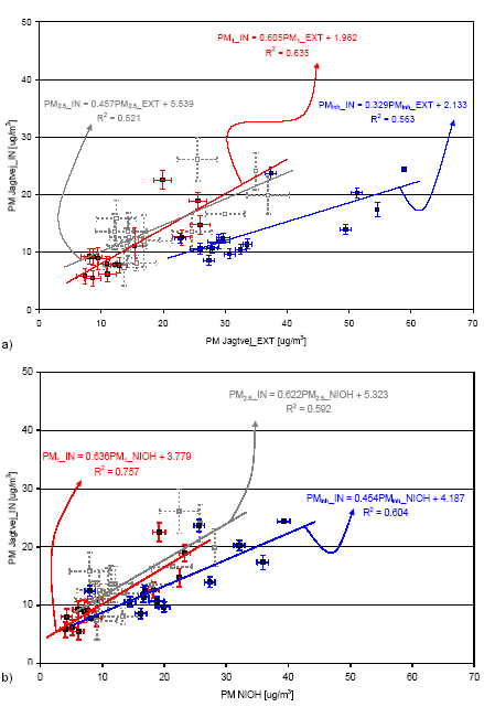
£ The artificial door to the sealed off kitchen was open the last 24 h.

$ Ventilation slits moved from the living room window to the bedroom window facing the backyard.

§ The air-exchange rate was uncontrolled and not monitored.

σ Standard deviation

Compared to a previous study, the average I/O-ratio for PM₁ was slightly lower than that observed in the same apartment during May 15 – June 13 and October 10 – November 11, 2001 (0.89±0.33 μg/m³;. However, in Sharma's study the street data for PM₁ were collected at first-floor level at the National Environmental Research Institute's Jagtvej monitoring station located on the other side of the street ~500 m NNE of the apartment outside Jagtvej 108. Owing to predominant western winds in Copenhagen, the PM-levels at this monitoring station are generally lower than at the other side of the street where the measurements in this study were conducted. During the current measurement campaign, the wind direction was in the western and eastern quadrant 42% and 29% of the time, respectively. Additionally, the ventilation slits were not installed in the apartment before October 2001. Before, during the 2001 summer campaign, the outdoor air entered the apartment through a large tube placed in the living room window. Both of these circumstances are expected to be of significant importance for the I/O relationships determined.

3.1.4.2 Variation in I/O ratio with air-exchange rate

It was anticipated that the infiltration of outdoor air-pollution would vary as function of the air-exchange rate in the apartment. - Increased air-exchange rates were expected to result in higher I/O ratios. However, no clear relationship was observed between I/O-ratios, or indoor particle concentrations for that matter, with air-exchange rate. The indoor particle mass concentrations only varied as function of the particle mass concentrations in outdoor air. Hence, variations in the ventilation rates appear to have insignificant effect on the indoor particle mass concentrations in the apartment. This is further supported by the modeling results in Schneider et al. (2004), who showed that the penetration of outdoor particles in the size-range 0.5 to 4.0 m was controlled mainly by the outdoor particle concentration and the indoor to street façade pressure difference.

3.1.4.3 Variation in indoor PM with outdoor PM

Scatter plots suggest a strong relationship between the levels of indoor particulate air-pollution with particulate air-pollution outdoors (Fig. 3.4). Based on the discussion above regression statistics was employed for further analysis of the indoor-outdoor relationships. The variation in indoor PM mass concentration was compared against PM measurements in the street canyon (Jagtvej_EXT) and in the urban background (NIOH) for each size fraction:

18) PM₁_IN = 1.98+0.604PM₁_EXT (p = 0.001; R²=63.5%)

19) PM₁_IN = 3.78+0.636PM₁_NIOH (p = 0.001; R²=75.7%)

20) PM_2.5_IN = 5.54+0.457PM_2.5_EXT (p = 0.004; R²=52.1%)

21) PM_2.5_IN = 5.32+0.622PM_2.5_NIOH (p = 0.001; R²=59.2%)

22) PM_inh_IN = 2.14+0.329PM_inh_EXT (p = 0.002; R²=51.1%)

23) PM_inh_IN = 4.19+0.454PM_inh_NIOH (p = 0.001; R²=60.4%)

It is clear that the indoor PM-levels can be predicted from outdoor particle concentrations with a relatively high probability for all three size-fractions measured. However, due to the high degree of mixing between the particulate air-pollution at Jagtvej and in the urban background (Fig. 3.2), it is unclear, whether the particulate air-pollution in the street or in the urban background has the greater influence on the indoor air from the direct regression analysis:

There appears to be a slightly better statistical relationship between the particulate air-pollution indoors and in the urban background. However, the I/O relationships using urban background data are unexpectedly high for PM₁ and PM_2.5 exceeding unity eight times. For comparison, the I/O ratio only exceeded unity three times when street data were used (Table 3.4). The high I/O ratios may be explained by episodic influence from indoor sources or indirect outdoor to indoor pathways. Indoor sources and indirect pathways have previously been suggested to play an important role on the fine and ultrafine particle concentrations in the apartment . However, it is not likely that the indoor sources would contribute with so much particulate air-pollution that the indoor PM₁ and PM_2.5 would exceed the outdoor air-pollution. Therefore, the apparent conclusion is that street air does have a significant influence on the indoor air pollution.

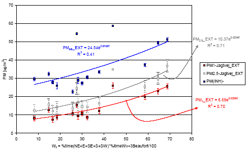
Figure 3.4: Scatter plots showing the relationship between the particulate air-polltion indoors and outdoors. a) PM₁, PM_2.5 and PM_inh indoors vs. corresponding PM₁, PM_2.5 and PM_inh at Jagtvej. b) PM₁, PM_2.5 and PM_inh indoors vs. corresponding PM₁, PM_2.5 and PM_inh at NIOH.

Analyzing the relationship between I/O values with the levels of particulate air-pollution and meteorological conditions show that high I/O ratios mainly occur when the air-pollution levels are low (Fig. 3.5). Low outdoor air-pollution levels generally occurred at high wind velocities and when the wind approached from the eastern and southern quadrants. In fact, the particle concentration showed a strong relationship with an empirical wind-factor (Wf) based on percent of time the wind velocity was below 3 Beaufort times the percent of time the wind direction was between NE and SW (Fig. 3.6). A similar trend was observed for PM in the urban background. This relationship may be explained by the fact that low wind velocities result in accumulation of traffic generated air-pollution in the street, whereas long-range transported air-pollution from Eastern and Central Europe generally are transported along air masses from South and East.

The relatively strong relationship between the Wf and I/O ratios suggest that meteorological conditions may play an important role on the particle penetration efficiency and penetration routes in the studied apartment complex. Especially elevated wind velocities could create complex pressure systems at Building facades and establishment of passage through alternative routes and/or enhancing transport of air-masses vertically in the Building complex. Further studies are required to understand these relationships in detail.

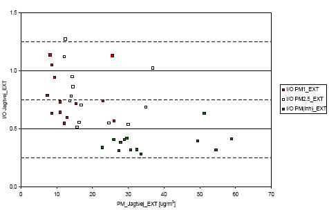
Figure 3.5: Scatter plot showing the relationship between the I/O ratio and the PM concentrations at Jagtvej_EXT.

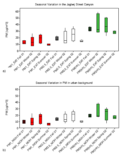
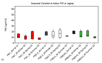
Figure 3.6: Variation in the particulate air-pollution in the Jagtvej street canyon with a combined wind direction and wind velocity (Wf) factor. The exponential regression equations were chosen based on visual best fit. Atmospheric data are listed in Appendix A.

3.2 Seasonal variation and comparison with PM guidelines

3.2.1 Seasonal variation

The collected and modeled data allows an evaluation of the seasonal variation in the particulate air-pollution levels in Copenhagen (Tables 3.5-3.7). To ensure comparison between the size-fractions, for all seasons, the summer season of was calculated based on four weeks only, omitting the NIOH data from the May 23-29, 2002 (Table 3.3). Despite predicted with high confidence (95%), the Fall '01 concentrations of PM_2.5 and PM_inh must be considered with caution as all data for that season are modeled.

Table 3.5: Seasonal and annual median and means for PM₁, PM_2.5 and PM_inh at Jagtvej_EXT

Click here to see Table 3.5

Table 3.6: Seasonal and annual median and means for PM₁, PM_2.5 and PM_inh at NIOH

Click here to see Table 3.6

The seasonal variation in the PM air-pollution is plotted in Figs. 3.7a to 3.7c representing each site. In the Jagtvej street canyon as well as in the urban background, all size fractions reached a maximum median PM concentration during the spring 2002 (EXT: PM₁ = 19.46, PM_2.5 = 25.54 and PM_inh = 37.38 μg/m³ and NIOH: PM₁ = 18.26, PM_2.5 = 21.38 and PM_inh = 25.63 μg/m³). At both of these outdoor locations, however, PM_inh had higher maximum concentrations during the winter 2002 (Tables 3.5 and 3.6; Fig. 3.7). This may be caused by higher amounts of traffic-generated air-pollution such as brake wear and resuspended dust (soil as well as sand and de-icing salts) from the road during wintertime. Increased effects of low wind velocities and long-range transport from eastern and middle-eastern Europe may also have an effect as indicated by the relationship between the wind factor (Wf) and PM levels in Fig. 3.6. Indoors, the maximum medians were observed during fall 2001 (PM₁ = 12.15, PM_2.5=16.23 and PM_inh=18.12 μg/m³) and spring 2002 (PM₁ = 12.60, PM_2.5=16.66 and PM_inh=13.95 μg/m³).

Figure 3.7: Seasonal variation of PM₁, PM_2.5 and PM_inh using both measured and modelled data. a) PM in the Jagtvej street canyon (EXT); c) PM in the urban background (NIOH); and c) PM indoors at Jagtvej (IN). Data from Fall '01 were obtained from Sharma (2002). The box plots show the median value, the upper and lower interquartile range and the 95% confidence interval for the interquartile range.

Table 3.7: Seasonal and annual median and means for PM₁, PM_2.5 and PM_inh at Jagtvej_IN

Click here to see Table 3.7

3.2.2 Comparison with air-pollution guidelines

Table 3.8 summarizes selected air-pollution guidelines. Currently, the Danish Environmental Protection Agency (DK-EPA) operates based on a limit for 24-hour average TSP concentrations (Total Suspended Dust) of 150 μg/m³. However, the EU has established a 2005 limit allowing a yearly average of 40 μg/m³ PM₁₀ and maximum 24-hour average of 50 μg/m³ that may be exceeded up 35 days per year. This limit will be further strengthened in 2010, where the annual average PM₁₀ concentration must not exceed 20 μg/m³ or exceed a 24h-average of 50 μg/m³ more than 7 times.

No EU-regulation has been developed for PM₁ and PM_2.5. However, American Environmental Protection Agency (US-EPA) have currently a guideline for a yearly average PM_2.5-concentration of 15 μg/m³, which the ASHRAE (American Society of Heating, Refrigerating and Air-conditioning Engineers) also suggest for indoor environments in the USA (Table 3.8). The EU, however, has formed a working group for establishing revised European air-pollution guidelines, including a guideline for PM_2.5 . This so-called CAFE working group has suggested that the future European guideline should not exceed an annual average PM_2.5 of 20 μg/m³ and a 90 percentile above 35 μg/m³ (Table 3.8).

Table 3.8: Selected National and International Air Quality Standards

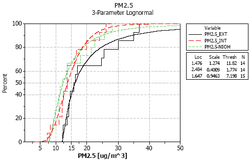
AM = Arithmic mean

£ Larssen et al. (2003) Air pollution in Europe 1990-2000, Topic report 4, EEA

$ www.epa.gov/airs/criteria.html

§ The guideline also accounts for indoor environments

z The EU CAFE Working Group on Particulate Matter recommends that an annual limit value should not exceed 20 μg/m³ and considers 12 to 20 μg/m³ as input for further assessment. The 35 μg/m³ is recommended as a reasonable starting point for a 24-hour limit.

Assuming that the average mass-concentrations represent the annual variation, the urban background concentration of PM_2.5 (14.85 μg/m³) was within the region of the EU-CAFE limit value proposals of 12 to 20 μg/m³ and just below the USA-EPA limit of 15 μg/m³. For comparison the average PM_2.5 concentration in the street was 19.80 μg/m³. Hence, the average street concentrations exceed the US-EPA annual average and all, but the maximum, EU-CAFÉ limit value proposals.

Whether there is a risk of exceeding the 24-hour PM_2.5 guideline was assessed by statistical analysis. The empirical distribution function analysis showed that the PM data could be described well with a 3-parameter lognormal distribution function. Fig. 3.8 shows the cumulative frequency plot and the distribution function for PM_2.5 at all three sites. The 3-way distribution function was chosen above the lognormal distribution function (P-value 0.026), because the 3-way function generally showed better fit and also defines a minimum threshold value based on the observed data. This prevents overestimation of low-concentration data.

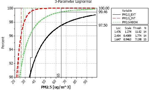
Figure 3.8: Cumulative histogram plot and the corresponding empirical 3-parameter lognormal distribution function for PM_2.5_EXT, PM_2.5_IN and PM_2.5_NIOH.

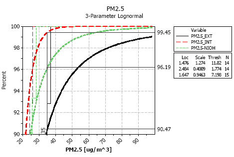
Figure 3.9: Percentiles for the 65 μg 24-hour limit on the empirical 3-parameter lognormal distribution function for PM_2.5_EXT, PM_2.5_IN and PM_2.5_NIOH.

Currently, the US-EPA requires that the 98% percentile of the 24-hour PM_2.5 concentrations is 65 μg/m³ or less. I.e., the average PM_2.5 cannot exceed 65 μg/m³ more than seven days during a year. Based on the distribution functions for PM_2.5, more that 99% of the PM_2.5 concentrations were below 65 μg/m³ in both the indoor and urban background air in this study (Fig. 3.9). In the street canyon, the PM_2.5 concentrations were statistically higher than 65 μg/m³ 2.5% of the time (9 days) in 2002 and hence exceeded the seven-day limit (Fig. 3.9). Despite, the estimates at the maximum concentrations drastically exceed reported values, a weekly average PM_2.5 concentration of 60.23 μg/m³ was measured in the urban background at NIOH during March 27 and April 4, 2002 during sampling on Teflon filters; outside of this project. This suggests that the statistical estimates presented are not unlikely.

Compared to the EU-CAFE proposal for PM_2.5, the PM_2.5 concentration at 4^th floor height at Jagtvej would be below 35 μg/m³ 90.47% of the time, hence just satisfying the potential EU 24-hour guideline (Fig. 3.10). Similarly, the annual average PM_2.5 EU-proposal of 20 μg/m³ was just satisfied in the street at Jagtvej (19.80±7.66 g/m³). In the urban background, the PM_2.5 concentration was below 35 μg/m³ 96.16% of the time and clearly complied with the potential future guideline.

Figure 3.10: Percentiles for the 35 μg 24-hour limit on the empirical 3-parameter lognormal distribution function for PM_2.5_EXT, PM_2.5_IN and PM_2.5_NIOH.

The average indoor PM_2.5 air-pollution (15.20±5.04 μg/m³) in the uninhabited apartment slightly exceeded the ASHRAE recommendation of 15 μg/m³. Regarding regulation of the particulate air-pollution in the indoor environment and considering that the apartment in this study was uninhabited, the results suggests great difficulties in compliance with the ASHRAE guideline for indoor environments and that susceptible people living at Jagtvej frequently may suffer from respiratory symptoms.

3.3 Evaluation of particle induced health effects

Increased concentrations of atmospheric air-pollution can result in acute health effects, such as increased rates of hospitalization owing to respiratory symptoms and cardiovascular disease as well as increased daily mortality. Long-term effects of air-pollution also occur and include increased risk of early mortality, respiratory morbidity and cancer related to long-term exposure to specific toxic compounds in the air .

Several studies have reported strong relationships between the incidence of acute or accumulated chronic health effects and increased 24-hour concentrations of especially PM₁₀ and PM_2.5 (e.g., Künnzli et al., 2001; Schwartz et al., 2001; 2002; Pope et al., 2002; Nafstad et al., 2004). The dose-response relationships are linear, at least up to several hundred μg/m³ of PM₁₀ and the response, here exemplified by acute daily mortality, is much stronger for PM_2.5:

24) %Incr_{AcuteMort-WHO2.5} = (0.151±0.039)PM_2.5)

than for PM₁₀

25) %Incr_{AcuteMort -WHO10} = (0.070 ±0.012)PM₁₀,

where %Incr_{AcuteMort-WHO} is the percent increase in mortality per million as function of the 24-hour mass dose of the respective PM measure in μg/m³ given by the WHO (2000). The stronger effect from PM_2.5 is in accord with the higher deposition efficiency of PM_2.5 in the lower human respiratory tract as compared to PM₁₀. The higher dose-response relationship for PM_2.5 also suggests that assessments based on PM₁₀ may underestimate the number of outcomes in regions if the atmospheric air-pollution is strongly dominated by fine particles.

Previously estimated the number of several health effects associated with atmospheric air-pollution in Denmark based on PM₁₀. They concluded that 435 extra deaths would occur per million adults above 30 years age (30+) in Denmark, including long-term effects, per 10 μg/m³ increase in PM₁₀. This mortality rate was determined at 7.5 μg PM₁₀/m³ resulting in a baseline of 10,122 deaths per year/million inhabitants. The corresponding number of excess hospitalization events for respiratory symptoms were 281 cases per million at a baseline of 14,670/year/million inhabitants.

3.3.1 Assessment of adverse health effects related to PM_2.5

In relation to this study, Relative Risk (RR) estimates only exist for 24-hour PM_2.5 measurements. Using the 7-day measurements, collected in this study directly, would result in underestimation of the maximum dose-response effects as compared to estimates using the corresponding 24-hour measurements. Applying the statistical distribution in mass-concentration from the 3-parameter lognormal distribution in Fig. 3.8 should minimize the risk of errors in the assessment of maximum and minimum acute dose-response effects. Moreover a statistical minimum value could be established, which is required for baseline calculations (Rate-PM_2.5base in equation 26). Consequently, the health effect assessment was made based on the statistical distribution of PM_2.5 in the urban background (Fig. 3.8). The variation was determined by converting the cumulative distribution frequency to number of days a year the air-pollution was below a specific PM_2.5 level, assuming that the statistical range reflected the 24-hour variation (Table 3.9). The statistically determined lower 24-hour PM_2.5 concentration of 7.57 μg/m³ was used to establish the baseline for the health effect assessment at which the contribution from urban air-pollution was assumed negligible. The statistical upper 24-hour PM_2.5 concentration of 79.12 μg/m³ was chosen as the maximum air-pollution level in the adverse health effect calculations (Table 3.9).

The effects on human health were assessed from published RR values for acute and accumulated (all cause) mortality, and for effects on acute hospitalization rates for cardiovascular and respiratory disease, respectively. The accumulated mortality includes deaths in relation to long-term exposure. Results are given as the number of incidents per million inhabitants per 10 μg/m³ PM_2.5. Health effect and population data used in the assessments were retrieved from Statistics Denmark (http://www.statistikbanken.dk) for the years 1999, 2000 and 2002 and listed in Table 3.10. The only exception was the 2002 data for mortality, which was estimated from the total number of deaths in 2002 using the average percentage of non-violent deaths in 1999 and 2000 (range 73.0±0.8% to 75.5±0.6% for the different population groups). Disease and mortality data were collected for Denmark as a whole and the Copenhagen and Frederiksberg Counties in the central part of Greater Copenhagen. The national population data (total population 5,313,577 to 5,368,354) were retrieved to test for abnormal variations in the Copenhagen data (total population 581,309 to 591,853). No sudden abnormalities were observed. However, higher disease and mortality rates were generally observed in the Copenhagen population.

Table 3.9: Cumulative distribution of the statistical PM_2.5 concentrations in the urban background (PM_2.5_NIOH) and method for conversion from cumulative distribution to time (t) mid mass distribution (PM_2.5mid).

In the first step of the assessment, the base level rates (Rate-PM_2.5base) were determined from equation 26 where the number of incidents per million inhabitants at the lowest air-pollution level was calculated:

26) Rate-PM_2.5base = N_obs/(1+[(RR-1)((PMave- PM_2.5base)/10 g/m³)]),

where N_obs is the observed number of incidents per million, RR is the relative risk estimate per million inhabitants per 10 μg/m³ increase in PM_2.5, and PM_2.5base (7.57 μg/m³) is the minimum PM_2.5 level. The number of cases per million per 10 μg/m³ (N-PM_2.5) was subsequently estimated from equation 27:

27) N-PM_2.5/10g/m³ = (RR-1)Rate-PM_2.5base

3.3.2 Increase per million per 10 g/m³ increase in PM_2.5

Table 3.11 lists the results from the assessment of acute mortality and cumulated mortality as well as the acute hospitalization rate for respiratory (Resp.) and cardiovascular diseases (CVD).

In all cases, the assessments for year 1999 and 2000 were conducted using PM_2.5 levels for 2002. Only the 2002 assessments were based on corresponding PM and health data sets. The results for the 1999 and 2000 assessments can only be used for evaluation of disease and mortality variations within the population.

Table 3.10: Data materials used for assessment of adverse health effects from PM_2.5.

Source: http://www.statistikbanken.dk

Filled cells = modeled data from percent of total mortality during 1999 and 2000

30+ denotes group of population at age 30 and above

The acute and total (all cause) mortality was estimated based on the average RR-value given by the WorL_D Health Organization, WHO (2000) and the 500,000 people metropolitan study from 1999-2000 by Pope et al. (2002), respectively. In the acute mortality, the RR value is based on the total age-range, whereas Pope et al (2002) estimated their RR-value for accumulated mortality in adults of 30 years age or oL_Der (30+).

The assessment of acute mortality suggest that the Copenhagen air-pollution may result in approximately 130 acute deaths per million Central Great Copenhagen inhabitants per 10 μg/m³ increase in PM_2.5 above the base level. Slightly lower effects (~120 ) were observed using national data (Table 3.11). The accumulated mortality including long-term health effects was notably higher and reached 721±480 and 833±555 per million per 10 μg/m³ increase in PM_2.5, using national and Central Great Copenhagen data, respectively. For comparison Palmgren et al. (2002) only predicted 435 deaths per million per 10 μg increase in PM₁₀. Assessment using PM₁₀ may underpredict the adverse health effects from particulate air-pollution the modern city environment. However, careful epidemiological studies are needed to verify this.

Table 3.11: Adverse health effect from PM_2.5 based on statistical urban background concentrations.

£ WHO (2000)

$ Pope et al. (2002)

§ Metzger et al. (2004)

Increased hospitalization rates for cardiovascular disease (CVD Hosp.) and respiratory symptoms (Resp. hosp.) are highly associated with increased levels of air-pollution. Metzger et al. (2004) determined a relative risk (RR) of 1.033±0.004 per 10 μg/m³ increase in PM_2.5 based on data from 4,407,535 all age emergency department visits in Atlanta (Georgia, USA) from 1993 to 2000. The average RR-estimate for increased hospitalization rates for respiratory symptoms (WHO, 2000) is slightly higher with a RR-value of 1.05 at a CI (confidence interval) of 95%.

The emergency visits for all CVD and respiratory symptoms reach 655±457 and 361 per million inhabitants in central Copenhagen per 10 μg/m³ increase in PM_2.5, respectively. The assessment of CVD and respiratory effects using national data (Table 3.11) results in similar rates as observed for Copenhagen (CVD=692±482; Resp.= 337).

3.3.3 Health effect assessment based on the PM_2.5 distribution function

In section 3.3.2. the adverse health effects were estimated as function of a 10 μg/m³ increase in PM_2.5. However, the expected number of adverse health effects is related to the actual exposure. To enable, an assessment of the number of cases related to specific air-pollution levels, the cumulative distribution function was converted to a time distribution function showing number of days with mid-point PM_2.5 levels (PM_2.5mid). The procedure to do this and the resulting time and PM_2.5mid data are shown in the right side of Table 3.9.

Thereafter, the number of incidents per million could be estimated using equation 28:

28) Nyear = Σ(Rate-PM_2.5base(RR-1)PM_2.5midt/365) for PM_2.5mid = 7.57 to 79.12

The 1-day upper and lower urban back-ground PM_2.5 level varied between 92.12 μg/m³ and 7.57 μg/m³ in the distribution function, respectively (Table 3.9). Assessment of the corresponding number of accumulated (all cause) daily deaths suggested an increase in up to app. 50% (= 117 people per million; Table 3.12). The corresponding maximum in excess hospitalizations for respiratory and cardiovascular disease reached was app. 25 (14±10 cases permillion) and 40% (8 cases per million), respectively.

Table 3.12: Range and total number of PM_2.5 dose-response effects in central Copenhagen.

£ Response effects were calculated with 95% CI based on the RR values listed in Table 3.11

Summing up over the year, the annual excess acute mortality was estimated 196±50 per million inhabitants in central Copenhagen (Table 3.12). The number of accumulated deaths were estimated as 780±520 per million inhabitants in the same population. Using similar technique, the predicted number of excess hospitalization events for CVD and respiratory symptoms amounted to 1006±701 and 554 per million Copenhagen inhabitants, respectively. Hence, in addition to approximately 800 early deaths, at least 1500 extra hospitalizations are expected to have occurred in Copenhagen per million inhabitants in 2002 owing to fine urban air-pollution.

| Front page | | Contents | | Previous | | Next | | Top |

Version 1.0 May 2005, © Danish Environmental Protection Agency