2 Methods

Buffer zones for biodiversity of plants and arthropods: is there a compromise on width?

In order to investigate the influence of buffer zone widths on biodiversity, we have tried to reduce the often challenging variation caused by using different farms over several years. Therefore, the whole experiment took place within one season at one large estate, Gjorslev Gods, on eastern Zealand. Gjorslev provided study facilities in four large spring barley fields with basically the same type of hedge composition with a herbaceous hedge bottom along the eastern side of the fields. The hedgerows had the same geographical orientation (north-south hedges). The size of the fields permitted the establishment of the necessary plot sizes within each field. The fertilization and spraying within the experimental plots was handled solely by the Farm Manager and one very experienced machine operator.

The biological work consisted of the following main parts:

Characterisation of the hedgerows (dimensions, composition of woody species and their flowering frequency)
Recording of all plant species in the fields and along the hedges, and in addition assessment of plant densities and flowering density.
Transect counting of selected insects such as butterflies and bumblebees.
Pitfall trapping of epigaeic beetles and spiders with focus on beneficials (natural enemies of pests).
Sweep net sampling of insects on plants designed to permit estimates of abundance, biodiversity and bird prey.
Beating tray samples of insects from hedges designed for obtaining abundance and biodiversity estimates.

Table 2. 1. Schematic summery of sampling times of wild flora and arthropods in hedge, hedge-bottom and field. Vegetation recording: 1) hedge dimensions, 2) hedge woody species composition, 3) hedge woody species flowering intensity, 4) coverage of hedge-bottom herbs 5) coverage of flowering and generative hedge-bottom herbs, field assessment of 6) number of Herbs and 7) number of flowering and generative Herbs. Arthropod recordings: 8) Pitfall trapping of epigaeic arthropods, 9) sweep net sampling of herbaceous dwelling arthropods, 10) transect counts of butterflies and bees and 11) arthropods sampled from woody hedge components.

Biotope	May, Period 1	June, Period 2	July, Period 3
Hedgerow	1, 2, 3, 11	3, 11	3, 11
Hedge-bottom	4, 8, 9	4, 5, 8, 9	4, 5, 8, 9
Field	6, 8, 9, 10	6, 7, 8, 9, 10	6, 7, 8, 9, 10

In Table 2.1 the sampling schedule of all data samplings is presented. Further details on the different methodologies are given in the subsequent sections of this chapter.

2.1 Study site and experimental design

The study was carried out as a single year field study at Gjorslev Estate in 2008.

2.1.1 Gjorslev Estate

Gjorslev Estate (Gjorslev vej 20, Holtug, 4660 Store Heddinge, Denmark, coordinates (wgs84): 55°21’14.34”N, 12°22’51.93”E) covers 1.668 ha of which 753 ha is forest. Gjorslev was asked to host the trial because of its large field sizes with well established homogeneous hedgerows. Large fields with long uniform hedgerows were needed in order to establish the required experimental design (section 2.1.2). An aerial view of a part of Gjorslev is presented in Fig. 2.1.

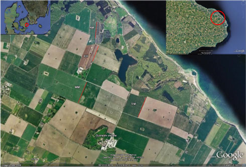
Fig. 2.1. Areal view of the four experimental fields At Gjorslev Estate: Møllemark (MM), Enghaven (EH), Anders mark (AM) and Skovmark (SM). The positions of the experimental parts of the hedgerows are indicated with red lines. The area is characterised by Large Fields in a relatively Heterogenous landscape with forest, lakes, running water and sea shore. As an indication of scale, the experimental area in Møllemark (MM) is 543 m long.

2.1.2 Experimental design

Four fields were included in the experiment (Fig. 2.1). In Fig. 2.2 an outline of an experimental field is presented. Data were collected on the western side of the eastern hedgerows in all fields. Along each hedge there were five treatments consisting of areas treated with neither fertilizer nor pesticides in 2008 – called buffer zones. The widths of the zones were 0, 4, 6, 12 or 24 m and they were arranged in chronological order for easier and more reliable management (Fig. 2.2).

Fig. 2.2. Outline of an experimental block within an experimental field. The trial included four such areas. There were five experimental plots within each block, each being 80 – 108.5 m long depending on the length of the hedgerow used in each field. The plot arrangement within a field was not randomized but was arranged at descending width of the buffer zone. However, within each field it was randomized whether the widest buffer zone of a field should be placed north or south. Five rows of sampling points perpendicular to the field edge were established for each experiment and were between 12.5 and 19.6 m apart depending on the plot length. The first and last sampling row within each plot was placed 15 m from the plot edge to lower interference from neighbour plots or ordinary field. Plant and arthropod sampling along each sampling row was carried out in the hedge bottom (ref. distance 0) and then 2, 5, 9 and 18 m within the field from the field edge (red squares). This sampling grid contained in total 25 sampling points per plot (5 × 25 = 125 pr. field). Additionally plant and arthropod recordings were carried out within the hedgerow.

The various buffer zones (treatments) are referred to as buffer 0 (0 m buffer), buffer 4 (4 m buffer) etc. It is important to emphasize that when the term “buffer 0 – 24” is used, it is the entire experimental plot area (in some cases at a specific distance from hedge) that is referred to and not only the width of the buffer strips (see Fig. 2.2). Hence, the size of the sampled area was always the same and it is only the ratio between treated and non-treated areas that varies.

The experiments were always surrounded by a section of ordinary field or headland. In both SM and MM the almost full length of the fields were included in the experiment and only guarded by 24 m of headland in both ends, as the field and the neighbour area on the western side of the hedgerow was fairly homogenous. In EH only the Northern end of the field was used, as the southern end was relatively low and often flooded during spring. This field was therefore guarded by 24 m of headland towards North and by approximate 200 m of field in the southern part. The experimental block in AM was placed along the middle of the hedgerow, thereby avoiding bordering up to a forest in the Northern part and a low waterlogged area in the Southern end. The experimental area AM was therefore bordered by 214 m toward North and 157 m toward South.

In SM and MM parts of the hedgerows had no trees or shrubs but herbs or grasses only. In SM this part was located in buffer 12 and comprised 30 m bordering to buffer 6. In MM buffer 24, 14 m were without woody plants. For more information on the hedgerows see section 3.1.1.

After randomization, the widest (24 m) buffer zone was placed at the northern end of the hedge in SM, MM and AM and at the southern end in EH. The plots in SM were 104.5 m long, 108.5 m in MM and 80 m in both EH and AM.

2.1.3 Pesticide and fertilizer applications

The four fields were treated identically with respect to the cultivation procedures, including fertilizing, sowing and pesticide application. The crop (spring barley cv. Henley) was sown relatively late in April due to wet soils. Right before sowing, liquid ammonia fertilizer was placed very accurate (injected) within the treated areas of the experimental plots. Later ammonium sulphate was applied (by rotary spreader) to the treated areas (for more information on fertilizer applications see Appendix A). Three weeks after sowing, a mixture of herbicides and fungicides was applied using low-drift (yellow) nozzles along with manganese sulphate. Eight weeks after sowing a mixture of fungicides and insecticides was applied (see Appendix A). Three weeks later, another insecticide treatment was carried out. The crop was harvested mid August (For more information on the pesticides and other field treatments see Appendix A). The pesticide dosages were normal according to the Danish Agricultural Advisory Service and close to the mean of 2008 (Miljøstyrelsen 2009).

2.2 Weather

The weather in spring (March, April and May) 2008 can be summarised as sunny and warm (dmi.dk/dmi/vejret_i_danmark_-_foraar_2008). The mean temperature in Denmark was 7.9ºC which is 1.7ºC above the average of the period 1961-90 but 1.1ºC lower than the same period in 2007. The mean precipitation in Denmark in spring 2008 was 131 mm which was 3 mm below the average of 1961-90. Denmark had 663 h of sunshine in spring 2008, which is the sunniest spring since the recording started in 1920.

The summer (June, July and August) in 2008 was sunny, wet and mild (dmi.dk/dmi/vejret_i_danmark_-_sommer_2008). The mean temperature in DK was 16.4ºC which is 1.2ºC above the average of 1961-90. The last half of July was very warm with several days above 25ºC. The mean precipitation was 240 mm which was 52 mm or 28% above the mean of 1961-90, although by far the highest amount of rain fell in August. Denmark had 721 h of sunshine in summer 2008, which is 130 h or 22% above the mean of 1961-90.

We measured the weather at Gjorslev using a local weather station (Hardi Klimaspyd) placed in the centre of the experimental field SM (Skovmark). These local weather data can be found in Appendix G.

2.3 Yield

The average barley yield in the experimental fields in 2008 was 72 hkg ha^-¹(79 hkg in SM, 72 hkg in MM, 76 hkg in EH and 59 hkg in AM). Yield losses within the buffer strips was not measured, however, according to the farm manager the yield in the buffer zones was assessed to be less than half the yield in the ordinary field (A.B. Hansen pers. comm.).

2.4 Vegetation recording

2.4.1 Hedgerow

Plant species composition of the hedgerows was assessed for all woody species and dominant herbs with 1 m resolution. The woody species were assessed once at May 7^th and the dominant herbs were assessed at three runs commencing May 7^th, June 19^th and July 17^th. The dimensions of the hedge were measured once at May 7^th with total height, height of bank and total width. Flowering intensity was determined for the dominant flowering woody species: May 7^th to 12^th for hawthorn (Crataegus spp.) and June 19^th for rose (Rosa spp.). Inflorescences (Crataegus) and number of flowers (Crataegus and Rosa) were counted on three 50 cm long branches in each plot. The value of the plants as pollen and nectar sources was recorded according to The Danish Beekeepers´ Association (Svendsen 1994).

2.4.2 Hedge bottom and field

In two sampling runs, 27 May - 12 June and 6 – 16 July respectively, vegetation was registered after the experimental fields had been sprayed with herbicides. At the distances 0, 2, 5, 9 and 18 m from the field edge (Fig. 2.2), 10 vegetation frames (Fig. 2.3) were used for density counts and for plant species (when possible) or genus recording according to Frederiksen et al. (2006). The frames were 40 × 50 cm², and divided into 20 sub-quadrants. Within the hedge bottom, density counts were not possible, and instead percent ground cover of each species/genus was recorded. At the second sampling run, flowering and generative stages of the plants were registered. The frames were always placed adjacent to one pit-fall (Fig. 2.3). Furthermore, 40 m from the hedge, 12 vegetation frames were sampled for additional information.

At the first sampling run, the number of spring barley plants was counted in all vegetation frames in four of the 20 sub-frames. The growth stage of spring barley was assessed according to the BBCH scale (Tottman & Broad 1987). Furthermore, the height and percentage cover of spring barley was registered, in treated and non-treated areas.

Click here to see: Fig. 2.3. The frames for wild flora registration (red squares). The frames in the hedge bottom and field were placed pair-wise with one pitfall for catching ground dwelling arthropods. A sampling point is indicated with a green spot. The sampling grid within a plot consisted of 25 sampling points (Fig. 2.2).Within the hedge bottom further spacing of the vegetation frames was needed because of the risk of flora damage when working with the pitfalls. Abbreviations for the four experimental fields: MM = Møllemark, EH = Enghaven, AM = Andersmark, SM = Skovmark.

2.5 Arthropod recording

Arthropod sampling was carried out in each of three sampling periods in 2008: Period 1 was after herbicide and fungicide application (May – early June). Period 2 was after the first insecticide and fungicide application (June – early July). Period 3 was after the second insecticide application (July).

2.5.1 Hedgerow

Arthropods were sampled on the woody plants of the hedgerows using a beating tray sampling technique. The sampling was carried out in May (28 May 2008), June (18 and 20 June 2008) and July (14 and 15 July 2008). Samples were collected in the five buffer zones per field along the west side of the hedges of the four experimental fields.

A beating sample was the sum of beating 1branch of 10 individual trees of the same species. Each branch received three firm beats. Arthropods were collected in plastic bags attached to the opening of the tray funnel. Samples were labelled with date, locality, buffer zone width, woody plant species and sample number.

The total number of samples per treatment was between 9 and 11 in order to accommodate that at least two samples were collected from each of the selected woody species present within a treatment (the average number of trees per combination of sampling time, field and buffer width was 9.6). In Andersmark, which was dominated by rose, it was not possible to obtain two samples pr treatment from the only other available species, hawthorn. The total number of samples was 576.

The faunal composition and total number of arthropods depends on the woody plant species. To obtain a correct picture of changes over time, and to be able to compare data from different treatments and fields, arthropods were only collected from the most common woody species available for sampling (it must be possible to reach and beat branches) in the four fields. In three of the fields, the woody species sampled were blackthorn (Prunus spinosa), elderberry (Sambucus nigra) hazel (Corylus avellana) and hawthorn (Crataegus spp.). However, the hedgerow of the fourth field, Andersmark, was strongly dominated by roses (Rosa spp.), with a few hawthorn interspersed, and only these two species were sampled in this hedgerow. Though present, it was not possible to sample from roses in the other three fields, as the roses in these fields were growing inside the hedgerow, and were not accessible for sampling.

Samples were kept in cooling boxes in the field. Cooling boxes maintained samples near 12^oC, hereby reducing deterioration as well as arthropod activity, hence the risk of predation in the samples. In the laboratory samples were kept at -20^oC until sorting and identification to order, family, genus or species under the stereomicroscope (see Table C.1 in Appendix C). All arthropods were named according to Fauna Europaea 2009 (http://www.faunaeur.org/index.php).

For important bird food items, the fresh weight was determined as a quantitative measure of the amount of bird food. For details on arthropod prey included as bird food see section 2.5.2.2.

For each sample, the woody species was recorded and the number of arthropod species was counted. The number of species was summed over the samples in each plot and Shannon’s indexes were averaged over the trees in each plot. Shannon’s biodiversity index was calculated for each combination of sampling time, field and buffer width (see section 2.6).

2.5.2 Hedge bottom and field

Three different sampling methods were used in order to cover arthropod populations of flying (avian), herbaceous dwelling and ground dwelling (epigaeic) species.

2.5.2.1 Transect counts of butterflies and bees

Standardized transect counts of Lepidoptera (butterflies) and Apidae (bees) were carried out following a method by Pollard (1977) and Pollard & Yates (1993) in order to estimate the activity of these insects in relation to buffer zone width.

Insect counts during systematic walks along the fields (transects) were carried out 2, 5, 9 and 18 m from the field edge. The 2 m distance census area was 4 m wide. It covered the hedgerow and 4 m into the field. In the relatively narrow 4–6 m strip (see Fig. 2.2) the census area was only 2 m wide. At the 9 and 18 m distances the census area was 4 m wide. In all cases the census area in front of the observer was 5 m long. The order of field visits, the starting points of the transect walks (North or South) and the order of the starting distance from the field edges were all randomised. Care was taken not to count an individual more than once, however, in doubtful cases or if an individual came from behind of the observer, it was always counted as a new individual. If the identity of an individual was uncertain, it was caught with a butterfly net and identified to species.

The observer spent 5 – 15 minutes walking through each census area of a plot. The time spent for each plot within a field was kept approximately uniform and was always registered.

Transect counts were preformed during three periods with three or four replicates in each of the four fields. Period 1: 27 May to 4 June. Period 2: 25 June to 11 July. Period 3: 24 – 31 of July. In total 40 transect counts were carried out. The earliest transect count began at 10.37 and the latest transect count ended at 18.14 (Greenwich Mean Time + 2 h). Wind speed (m/s at 24 m from the hedgerow), sunshine (on a scale from 0 – 4 with 0 representing full sun and 4 completely clouded) and temperature (ºC) were all registered. The wind speed never exceeded 6.5 m/s and the temperature was always above 17 °C during transect counts. If rain set in, the counting was abandoned and a new attempt was made the next day. During each period, one set of transect walks were completed in each of the four fields before starting the next sampling round. Each round lasted no more than three days.

2.5.2.2 Sweep net sampling of arthropods in the herbaceous vegetation

Herbaceous-dwelling arthropods like butterfly larvae and leaf beetles were sampled using standard sweep nets (diam. 27 cm). One sample (10 standard sweeps) was taken at each of the 25 sampling points per plot (see Fig. 2.2) on three occasions. The first sampling occasion was 2-3 June, 12-13 days after herbicide and fungicide applications. The second sampling round was carried out 24-26 June, 7-9 days after the first insecticide and fungicide application. The third and last sampling occasion was 15-16 July, 13-14 days after the second insecticide application. In total 1500 sweep net samples were collected.

The catch from each sample was put in a plastic bag, labelled and placed in a cooling box until it was frozen at -20ºC later the same day. In the laboratory all arthropods were counted and identified at least to order. The majority of, taxonomic units were identified to species (see Table D.20 in Appendix D). All arthropods were named according to Fauna Europaea 2009 (http://www.faunaeur.org/index.php).

Chick-food items

In order to identify buffer zone effects on the availability of arthropod food for higher trophic levels, arthropods being important as chick-food (see Wratten & Powell 1991, Sotherton & Moreby 1992, Petersen & Navntoft 2003) from the sweep net samples were grouped and weighed per sample (g fresh biomass after de-frosting): Araneae, Opiliones, Coleoptera (except Coccinellidae and Cantharidae), Hemiptera, Lepidoptera (larvae only), Tenthredinidae (larvae only), Syrphidae (larvae and pupae only), Orthoptera and Neuroptera.

2.5.2.3 Pitfall trapping of epigaeic arthropods

Carabidae (ground beetles), Staphylinidae (rove beetles), Araneae (spiders) and other epigaeic arthropods were sampled with pitfall traps (plastic cups, diameter 82 mm, depth 70 mm, with snap-on lids) buried flush with the soil surface. The traps were partly filled with 200 ml of trapping and preservation fluid (a mixture of 1:1 ethylene glycol and tap water, with one drop of non-perfumed detergent per 10 l). In total 25 traps were used per plot (see Figs. 2.2 and 2.3). Three sampling rounds were carried out. The first set of traps were started 28 May (six days after herbicide application, see Appendix A for pesticide details). The second set of traps was started 18 June (one day after the first insecticide application) and the third set of traps was started 11 July (nine days after the second insecticide application). The first sampling round lasted 48 h and the second and third 72 h before the traps were collected, labelled and stored at 5°C until further processing. In total 1500 pitfall samples were collected. In the laboratory arthropods belonging to Araneae (spiders), Carabidae (ground beetles), Staphylinidae (rove beetles) and a few other taxa were counted and identified at minimum to family but preferably to species (see Table D.24 in Appendix D)

2.6 Data analysis

In addition to the actual recorded number of individuals, two measures were calculated in order to access the biodiversity: The number species (species diversity) and Shannon´s biodiversity index, H (Magurran 2004). Shannon´s H was calculated as:

Formula

Both measures were calculated and analysed for selected groups of plants and arthropods.

In order to estimate and test the effects of buffer width, distances from hedge and in some cases sampling time, the data were analysed statistically. The applied statistical methods and models depended to a large extent on the type of data, so that linear mixed models were used for data that could be assumed to be normally distributed such as weights, Shannon´s biodiversity index and log-transformed number of species, while counts and relative counts that could be assumed to be Poisson distributed and binomial distributed, respectively, were analysed using generalised linear mixed models. The random effects included in the models reflect that each field could be regarded as a complete block (replicate) in the same experiment – an experiment that is regarded as a split-block design. The actual applied models are explained, shown in a mathematical form and listed in Appendix F. In the following, the models are described very briefly with reference to the detailed description in Appendix F. The theory of linear mixed models and generalised linear mixed models may be found in books such as McCulloch and Searle (2001) and West et al. (2007). All statistical analyses were performed using the procedures MIXED, GLIMMIX and NLMIXED of SAS (SAS, 2008). Some of the results were visualised using the graphical procedures of SAS (SAS 2009a and SAS 2009b).

2.6.1 Flora analyses

The number of counted plants at each sampling period was analysed using generalised linear mixed models. The analyses were carried out for the different sampling period and groups (all, type and family) of plant species. The fixed effects in the model depended on the source of the data: field or hedge. For data from the hedge the model included the fixed effect of field and buffer width (Model 6 of Appendix F). For data from the field the model included the fixed effect of field and buffer width, distance to hedge and the interaction between buffer width and distance (Model 8 of Appendix F). The data from the field were also analysed in models, where the effect of buffer width and distance to hedge were treated as continuous variable using a second degree model (Model 12 of Appendix F). This model was then subsequently reduced by removing non-significant effects in order to get a model as simple as possible. The percentage of flowering plants at the second sampling run were analysed using a generalised linear mixed model including the effect of field and buffer width, distance to hedge and the interaction between buffer width and distance (Model 9 of Appendix F). The percent flowering plants in hedge-bottom at the second sampling run was calculated from the sum over coverage of all plants and flowering plants for each combination of field and buffer width. The log-transformed values were analysed in a linear model including the effect of field and buffer width as fixed effects (Model 13 of Appendix F).

Shannon´s index and the number of species (after log-transformation) were analysed in different models. Initially the data were analysed in a linear mixed model. The effect of location (control recordings in “the middle” of the field versus plots close to the hedge) together with the following three effects: ¹⁾ distance to hedge, ²⁾ width of buffer zone and ³⁾ the interaction between distance to hedge and width of buffer zone. The model also included the effect of sampling period and interactions with sampling period (Model 14 of Appendix F).

In order to evaluate the distance at which Shannon's index was reduced to half its value at the hedge, the difference between its value in the hedge and its value in “the middle” of the field was also modelled using the logistic function. Two versions of the models were used: ¹⁾ where it was assumed that decrease per unit (log distance) were the same for all buffer zones and ²⁾ where it was assumed that decrease per unit (log distance) depended on the buffer zone (Model 5 of Appendix F).

2.6.2 Arthropod analyses

2.6.2.1 Hedgerow

The different groups of arthropods in the beating tray samples at each sampling period were analysed in a generalised linear mixed model including the fixed effect of field, buffer width and tree species (Model 7 of Appendix F) whereas the weights of bird feed at each sampling time were analysed using a linear mixed model including field, buffer width and tree species as fixed effects (Model 4 of Appendix F).

2.6.2.2 Hedge bottom and field

Transect counts of butterflies and bees

The number of individuals for different groups of arthropods were analysed separately for each sampling period using a generalised linear mixed model that included the fixed effect of field and buffer width distance to hedge and the interaction between buffer width and distance. In order to adjust for time spent in the transect, day and time of sampling and the other conditions for activity (e.g. temperature) the logarithm of the time spent in the transect was includes as an offset variable, the actual day was included as a fixed effect while the linear and quadratic effects of the following variables were included as covariates (fixed continuous effects): time of day (hours before or after noon), amount of sun (on a scale from 0 to 4 with 0 being full sun (no clouds) and 4 being fully overcast) and temperature (°C). This model was then reduced step by step by removing non significant covariates. The full model is Model 10 of Appendix F.

Shannon´s index (see section 2.6) and number of species (after log-transformation) for selected groups of arthropods were analysed using a linear mixed model including the fixed effects of buffer width, distance to hedge, sampling period and all 2- and 3-way interactions between these (Model 2 of Appendix F).

Sweep net sampling of herbaceous dwelling arthropods

The data were aggregated over replicates before analyses in order to decrease the number observations with zero target arthropods. Different groups of arthropods at different sampling periods were analysed using a generalised linear mixed model that included the fixed effect of field, buffer width, distance to hedge and the interaction between buffer width and distance (Model 8a in Appendix F).

The weight of bird feed at each sampling period were analysed in a linear mixed model including the fixed effects of field, buffer width, distance to hedge and the interaction between buffer width and distance (Model 3 of Appendix F).

Shannon´s index and number of species (after log-transformation) for selected groups of arthropods were analysed using a linear mixed model including the fixed effects of field, buffer width, distance to hedge, sampling period and all 2- and 3-way interactions between buffer width, distance to hedge and sampling period (Model 2 of Appendix F)

Pitfall trapping of epigaeic arthropods

The data were aggregated over replicates before analyses in order to decrease the number observations with zero target arthropods. Different groups of arthropods sampled were analysed separately at each sampling time using a generalised linear mixed model that included the fixed effect of field, buffer width, distance to hedge and the interaction between buffer width and distance (Model 8a of Appendix F).

Shannon´s index and number of species (after log-transformation) for selected groups of plants were analysed using a linear mixed model including the fixed effects of field, buffer width, distance to hedge, sampling period and all 2- and 3-way interactions between buffer width, distance to hedge and sampling period (Model 2 of Appendix F)

2.6.3 Combined flora and arthropod analyses

2.6.3.1 Activity of Lepidoptera (butterflies) and Bombus in relation to flower and host plant abundance

In order to evaluate the effect of plants on the occurrence of selected groups of arthropods, avian species from transect data were analysed in a second model. This second model included the same fixed effects as the model for transect data (Model 10 of Appendix F) together with linear and quadratic effects of the following variables: number of host plants (or coverage of host plants)and number of flowers for selected or all plant species (Model 11 of Appendix F). The full model was reduced step by step by removing non significant variables.

2.6.3.2 Analyses on the marginal gain of biodiversity when increasing buffer width

For wild plants and selected arthropods groups (Heteroptera, herbivorous coleopterans, Carabidae and Lepidoptera), the total number of species in each of the distances ranges 0, 0-2 m, 0-5 m, 0-9 m and 0-18 m was summarised for each combination of field and buffer width. Woody species in the hedge rows were not included in the plant analyses. Lepidoptera (butterflies) were not analysed for distance 0 m, as this distance was included in distance 2 m during data recording.

The number of species from each of those distance ranges were analysed in a linear mixed model (after log-transformation) including the effect of field and buffer width (Model 13 of Appendix F). These analyses were carried out on the July data comprising hedge bottom and field area (sampling run 2 for plants and sampling period 3 for arthropods) where the experimental plot had received the full fertilizer and pesticide effects.

The data for all buffer widths were also analysed in a non-linear model (Model 15 of Appendix F) to estimate the species – area relationship (SPAR). Arthropod data from the woody species in the hedgerows were included in the modelling, however, the distances in the hedgerow (hedge bottom versus hedge row) were analysed as one distance (dist. 0) in this model to make them fit into the assumed species – area relationship. The area for each distance was counted as the unit 1. Data were summarized across all sampling times in order to reveal buffer effects on biodiversity comprising the entire season.

2.6.3.3 Lepidoptera (butterflies) as bioindicator for biodiversity gains of buffer zones

The data for selected group of arthropods were analysed in a generalised linear model in order to examine the possible correlation between arthropod species diversity and species diversity between arthropods and dicotyledons. In order to avoid that the possible correlation was introduced by the difference between treated and untreated plots, the model include the effect of treatment as fixed factor as well as possible significant effect of field. The model also allowed the correlation to depend on whether the plots were treated or untreated (for more details see Model 16 in Appendix F).