Calibration of Models Describing Pesticide Fate and Transport in Lillebæk and Odder Bæk Catchment
3 Model Setup
- 3.1 Modelling water flow in the catchments
- 3.2 Modelling water flow in the stream models
- 3.3 Pesticide model for the catchment
- 3.4 Pesticide model for streams and ponds
- 3.4.1 Solar insolation
- 3.4.2 Dispersion
- 3.4.3 Suspended matter, temperature and pH
- 3.4.4 Biomass of macrophytes
- 3.4.5 Sediment bed
- 3.4.6 Sorption to sediment and suspended matter
- 3.4.7 Sorption to macrophytes
- 3.4.8 Biological degradation in pore water and water column
- 3.4.9 Biological degradation at macrophytes
In the following, a description is given of the specific data included in the Lillebæk and Odder Bæk models. As the final data choice in some cases builds on considerable analysis, the main issues are summarised in the following sections and the details are given in appendices.
3.1 Modelling water flow in the catchments
3.1.1 Discretisation
Both models are established in a 50-meter grid – i.e. each calculation cell measures 50x50 meter. Given the catchment areas to which the model areas where adopted the number of boundary cells and internal calculations cells equal (178/1849) and (243/3929) per layer for Lillebæk and Odder Bæk respectively. The vertical discretization is set to reflect the geological model – i.e. the calculation layers are set equal to the geological layers. For the unsaturated zone, the discretisation is fine near the surface and coarser towards the groundwater table. In Lillebæk the cell height is between 2.5 and 5 cm in the A and B horizon, and between 5 and 50 cm in the C horizon. In Odder Bæk the discretisation has not been strictly linked to the horizon but more controlled by the depth resulting in 2.5 to 10 cm cell height in the A horizon, 5 to 10 cm in the B horizon, and 20 to 50 cm in the C horizon.
3.1.2 Boundary conditions
In the upstream end of the Lillebæk catchment, water flows into the area since a groundwater divide can be identified outside the model area – found using a map of groundwater potentials provided by the county of Funen. In the downstream end outflow through a white sand layer is expected to take place towards the sea (Dansk Geofysik, 2000; DGU, 1989a). Where the groundwater flow is expected to take place across the boundary, boundary conditions are described using the option constant hydraulic pressure where. Furthermore, modifications had to be made for the sand lens (see the chapter on geological description, 3.1.6). Evaluating the extent of the lens, the surface topography and the topology of the Hammersbro Bæk just south of the Lillebæk model it is found that flow is likely to take place in the lens towards Hammersbro Bæk. For a proper boundary description knowledge of the potentials in the lens would be of most importance. No direct information is available and it was chosen to fixate the potential head in the lens east of Oure town – over 750 meters going from 34 m.a.s in west to 24 m.a.s. in east.
The boundary of the Odder Bæk model is slightly modified compared to the surface catchment area. To the north the boundary is adjusted to match the groundwater divide. From the two hydro-geological reports (DGU, 1989b, Nordjyllands amt, 1998), the following assumptions with regard to groundwater were adopted:
- Groundwater flow in the upper aquifer is most likely routed towards the stream
- The lower aquifer has a larger extent than the small Odder Bæk stream catchment and groundwater flow is assumed flow from north to south.
- There may be contact between the two aquifers in parts of the catchment
- Based on head observations in the upper aquifer, it is likely that an east-west groundwater divide is located north of Gislum.
By running the model with different boundary conditions the most probable direction of groundwater flow in the upper aquifer was estimated. In this way, the model itself was used to establish the most probable groundwater catchment for the upper aquifer, and a new catchment was established which are smaller than the topographical catchment and more smooth around the corners (Figure 3.7).
Finally, the southern border was opened to allow water to move towards the stream to the south. This last change is in correspondence with a map of hydraulic potential made available by the county of Northern Jutland and improved the simulations of groundwater variations in the southern part of the Odder Bæk catchment.
3.1.3 Climatic variables
The choice of climatic parameters is not entirely consistent. This is mainly caused by several changes in recommendations from the concerned institutions over the time of the project, and differences in data availability in the two catchments.
For Lillebæk, precipitation is measured in the catchment during the whole period of the project (station: Bolsmose). In addition, rainfall intensity (per 15 minutes) is measured at a special station in the catchment from mid 1999 till the present. The measurements of precipitation are corrected, using the (new) standard correction factors (Allerup et al., 1998). Climatic parameters for calculation of evaporation are measured at a nearby research station (Aarslev). Evaporation is calculated according to Makkink (Aslyng and Hansen, 1982).
It should be noted that the Lillebæk catchment and the drain stations have been the object of other model studies. An analysis of earlier simulations for the catchment showed considerable differences between climatic datasets chosen, partly due to selection of different data sources and partly due to errors in the data sets. The results presented here are therefore not necessarily similar to what has been presented earlier from NOVA (the National Monitoring Programme).
For Odder Bæk, the choice of climatic data went through several iterations, see Appendix A. The precipitation record finally selected is grid precipitation from DMI for grid no. 10215, modified with the correlation (P = 0.926 * Pgrid, R2 = 0.96). This generated series is then corrected, using the dynamic correction factors from Vejen et al. (2000) and (2001). Evaporation is calculated according to Makkink, for the same grid.
Due to the fact that macropores are included in the description in Lillebæk, data from the rainfall intensity station 28184 on Funen was analysed. It is the intensity station that resembles the Bolsmose station the most. Data was summarised for every 6 minutes, and the record corrected so that the monthly rainfall is identical to the rainfall at the Bolsmose station. This is not entirely correct, because one of the differences between the station types is that very small events are not measured by the intensity stations. With this correction method, the lacking rainfall is added to the measured events through scaling of the measured events. It was, however, the only possible way to create a record with realistic intensities for the whole of the measurement period. This high intensity rainfall was only used in the scenarios, while the calibration of the water flow was done on daily values. For the calibration of pesticide transport, however, the model was run with the intensity record in order to generate macropore flow and colloids.
3.1.4 Vegetation parameters
Within the two catchment areas of forest, wetlands, urban/fallow and arable lands were mapped. In the arable lands different crop are represented – winter cereal, spring cereal, pea, beet, potato, and grass – and randomly distribution of the crops was performed.
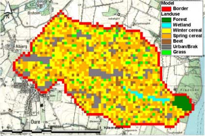
Figure 3.1 Distribution of vegetation in the Lillebæk model.
Figure 3.1 Arealanvendelsen i Lillebæk-modellen.
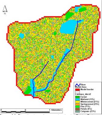
Figure 3.2 Distribution of vegetation in the Odder Bæk model.
Figur 3.2 Arealanvendelsen i Odder Bæk-modellen.
The MIKE SHE water model requires data about the development of leaf area index and root depth for each crop or vegetation. These are derived from (Plauborg, F. Olesen, 1991) for the agricultural crops.
Inception and transpiration is described as a function of root depth, root distribution and leaf area index in the model. However, experience has shown that transpiration exceeds potential evaporation under certain conditions. To account for that, the potential evaporation is multiplied with 1.25 for permanent grass along the stream (wetland), and with 1.1 for crops during the period of maximum vegetative growth. This is in line with the general recommendations of FAO for calculation of evapotranspiration for crops, and it is believed to be in line with the new recommendations for calculation of evapotranspiration under Danish conditions (Plauborg et al., 2002).
3.1.5 Soil parameters
The sources of soil information for the two catchments are: Soil profile descriptions carried out for six profiles in each catchment (Nielsen, 1998, Nielsen, 1999, Jensen and Madsen, 1990), soil maps from Foulum ("Jordklassificering, Danmark, Basisdatakort, 1:50.000-JB 1312 11 NØ (Lillebæk) and similar maps made available by the County of Northern Jutland), soil type maps from GEUS describing the soil material in 1 m's depth, and to some extent information from geological boreholes and geophysical measurements of the two catchments.
For Lillebæk, the soil map of the plough layer is almost uniform for the whole catchment. The map of 1 m's depth shows sandy underground in the eastern end of the catchment. This corresponds well with the geological interpretation of the catchment in general and with the soil profiles described. The easternmost profile shows sand at depth. However, in spite of the fact that the catchment appears uniform on the maps, the hydraulic parameters measured differ from profile to profile. To catch the variation in the model, parameters from the 5 profiles analysed are distributed randomly in the uniform area, while parameters from the 6th profile are used for the area with sand at depth. Macropores are included in the description. They make up 1% of the volume of the soil. Key parameters for each soil are shown in Appendix B.
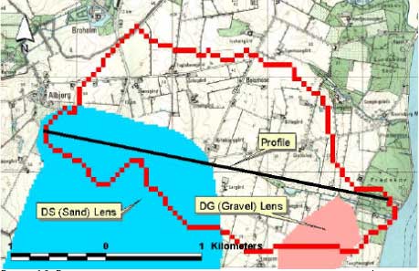
Figure 3.3 Map showing the distribution of the soil types used in Lillebæk and the locations of the measured soil profiles (St. 1-6). Profile 1-5 are distributed randomly, while profile 6 is used in areas where the geology indicates sand at 1 m's depth.
Figur 3.3 Kort over fordelingen af jordtyperne i Lillebæk og placeringen af de målte profiler (St 1-6). Profilerne 1-5 er tilfældigt fordelt mens profil 6 anvendes i den del af arealet hvor geologien indikerer sand i 1 m's dybde.
The interpretation of soil types in Odder Bæk was less straightforward. Topsoil parameters in terms of soil texture, retention curves and saturated hydraulic conductivity have been measured at 6 locations within the catchment (black dots on Figure 3.4 with measured top- and subsoil texture class (JB)). Comparing the measured data with the available map of topsoil classes shows that only 3 of the 6 measured data sets match the map classification. Some of the profiles show rather heavy textures at depth. To improve the understanding, an effort was made to interpret the geological borehole data of the area. A clay layer was identified which varies from 0.5 metre to 42 metre below the soil surface with a thickness varying between 1 and 26 metre. In addition, a local appearance of clay deposits close to the soil surface, oriented east-west, has been identified in the middle of the catchment. The thickness of this deposit varies between 0 and 15 m. The soil map finally generated is thus somewhat different from the original.
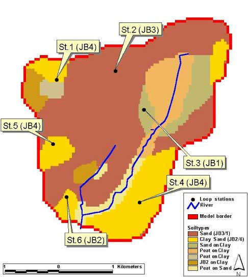
Figure 3.4 Map showing the distribution of the soil types used in Odder Bæk and the locations of the measured soil profiles (St. 1-6).
Figur 3.4 Kort over den anvendte jordtypefordeling i Odder Bæk og placeringen af de beskrevne profiler.
The hydraulic parameters used for the different zones were initially based on measured values, but some values were changed during calibration. Initially, the measured values from station 2 represented the soil type "Sand" but it was not possible to reproduce the measured variations in groundwater levels corresponding to the measured values with this rather extreme retention curve. The values finally selected are described in Annex B. No measurements were available to represent the organic soils present in the catchment. General parameters from literature were therefore used (Annex B).
3.1.6 Geological description and hydraulic parameters
For Lillebæk, the geology is described on the basis of geological borehole data from the ZEUS geological database. Secondly, during the spring 2000, the county of Funen mapped the area by means of geophysical measurements (Dansk Geofysik, 2000) providing an excellent extension of data available for geological interpretation. Thirdly, the utilisation of the geological interpretation tool, GeoEditor (DHI, Water & Environment, 2000), has made a simultaneous interpretation possible from both geological borehole information and geophysical data.
The interpretation has been conducted at DHI, but the County of Funen has played an important role in the verification of the model by providing geological experience along with previously interpreted profiles.
The adopted interpretation procedure was to import the borehole database in the GIS-based GeoEditor, and construct geological profiles. Three of the profiles match interpreted profiles by the County of Funen, another 15 of the profiles match geophysically interpreted (TEM) profiles by Dansk Geofysik (2000), and seven of the profiles were oriented west east to cover the overall area mainly with respect to the boreholes. The geological layers were afterwards interpolated on the basis of the digitised profiles.
A three-layered geological model was established – with a sequence from surface of moraine, white sand and tertiary clay. Two major lenses of sand and gravel are encapsulated in the moraine clay. The extents of the lenses are shown in , and a west-east cross section of the geological model is shown in . The upper sandy lens (a secondary aquifer) consists of diluvial sand, whereas the lower sandy (primary aquifer) consists of interglacial sand. The main orientation of the sandy deposits is horizontal. In most of the area the lower sandy aquifer is underlain by tertiary clay (Kerteminde mergel) forming an aquitard of very low permeability. The approximate location of the bottom of the lower sandy aquifer is 0-10 m below sea level. The thickness of the primary aquifer typically varies between 8 and 16 m, but increases to 20-30 m to the very west and decreases to 0 m to the very east of the area.
The hydraulic conductivities applied in the model are listed in .
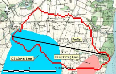
Figure 3.5 Extent of gravel and sand lenses in the moraine clay layer in Lillebæk.
Figur 3.5 Udbredelsen af grus- og sandlinser i morænelers-området i Lillebæk.

Figure 3.6 West-East geological profile in Lillebæk along the line indicated in Figure 3.5.
Figur 3.6 Geologisk profil i Lillebæk gennem linien vest-øst indikeret i figur 3.5
Table 3.1 Parameters applied for the geological formations in Lillebæk. For the top calculation layer the storage capacity values are automatically adjusted by values specified in the unsaturated zone.
Tabel 3.1 Parametre anvendt til beskrivelse af de geologiske formationer i Lillebæk. For det øverste beregningslag er porevoluminet automatisk justeret med værdierne specificeret for den umættede zone.
| Formation | Conductivity | Storage Capacity (-) |
Specific Yield (-) |
|
| Horizontal (m/s) | Vertical (m/s) | |||
| Moraine | 4.37e-6 | 4.37e-7 | 0.2 | 0.001 |
| White Sand | 1.36e-5 | 1.36e-6 | 0.3 | 0.002 |
| Tertiary Clay | 3.74e-6 | 7.48e-8 | 0.2 | 0.001 |
| Sand Lens | 8e-5 | 4e-5 | 0.3 | 0.002 |
| Gravel Lens | 8e-5 | 4e-5 | 0.3 | 0.002 |
With respect to Odder Bæk, the area is not well enough covered by deep boreholes to create a reliable geological model only from boreholes. Thus, geophysical data have been employed in the interpretation.
The geological model has been established on the basis of two reports on hydro-geological mapping (DGU, 1989b; Nordjyllands Amt, 1998), together with borehole data extracted from the geological database (ZEUS) at GEUS. The adopted interpretation procedure was to import the borehole database in a GIS-based GeoEditor, and construct geological profiles which as close as possible match 7 interpreted profiles, which are presented in the latter of the mentioned reports. The geological layers were afterwards interpolated on the basis of the digitised profiles.
The outcome of the process is a geological model with 2 sandy aquifers divided by a clay layer. The bottom of the model is the top of a thick clay layer located underneath the two sandy aquifers, approx. 20 m below sea level. In the geological reports a third deep aquifer has been identified (approx. 70 m below sea level), but as this will not be in contact with the stream, Odder Bæk, it has been excluded from the model setup. The position of the clay layer varies from 0.5 m to 42 m below surface with a thickness varying between 1- 26 metre. In addition, a local appearance of clay deposits close to the soil surface has been identified in the western part of the catchment – beneath a small lake. This deposit has been included in the model as a lens with specified extent – shown in and in cross section in Figure 3.8.
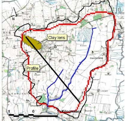
Figure 3.7 Extent of clay lens in the top sand layer in Odder Bæk. The black curved line shows the topographical catchment, while the red "box"-line shows the actual model area.
Figur 3.7 Udbredelse af lerlinse i det øverste sandlag i Odder Bæk. Den sorte kurvelinie viser det topografiske opland mens den røde "kvadrat-linie" viser det faktiske modelområde.
Figure 3.8 NWest-SEast geological profile in Odder Bæk along the line indicated in Figure 3.7.
Figur 3.8 Geologisk profil i Odder Bæk gennem linien nordvest-sydøst indikeret i Figur 3.7.
Table 3.2 Parameters applied for the geological formations in Odder Bæk. For the top calculation layer the storage capacity values are automatically adjusted by values specified in the unsaturated zone.
Tabel 3.2 Parametre anvendt til beskrivelse af de geologiske formationer i Odder Bæk. For det øverste beregningslag bliver porevoluminet automatisk justeret med værdier specificeret for den umættede zone.
| Formation | Conductivity | Storage Capacity (-) |
Specific Yield (-) |
|
| Horizontal (m/s) | Vertical (m/s) | |||
| Top Sand | 1.03e-5 – 1.25e-4 | 12/100*Kh | 0.3 | 0.0004 |
| Clay | 4.00e-7 | 8.00e-8 | 0.35 | 0.0005 |
| Bottom Sand | 2.00e-5 | 1.00e-5 | 0.3 | 0.0004 |
| Clay Lens | 1.4e-7 | 1.60e-7 | 0.35 | 0.0005 |
The overall impression of the geological interpretation is that the area is rather complex with respect to groundwater flow with clay deposits located near the soil surface in 15-25% of the area. The hydraulic conductivities have for the top sand been specified as distributed values, with a ratio between horizontal and vertical values of 100/12. The distribution is shown in Figure 3.9
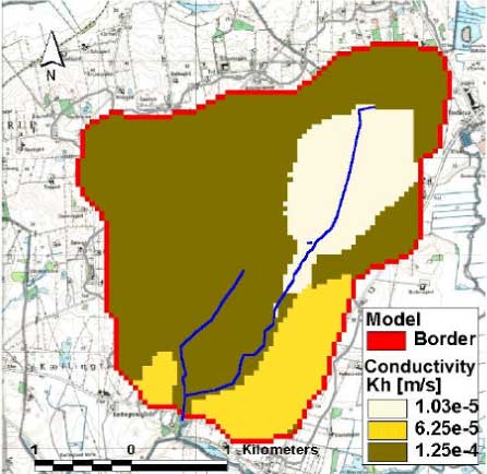
Figure 3.9 Horizontal conductivity in top geological layer in Odder Bæk. The vertical conductivity is set to 12/100 of the horizontal values.
Figur 3.9 Horizontal ledningsevne i Odder Bæk-oplandet. Den vertikale ledningsevne er sat til 12/100 af de horizontale værdier.
3.1.7 Drains
It was foreseen that drains were common in Lillebæk. Additionally, the stream is piped along most of its length. The "stream system" shown on Figure 3.10 is modelled in MIKE 11, as streams, while the drainage systems are modelled in MIKE SHE.
Drainage maps were received from the county of Funen. In the model drainage is implemented in almost the whole catchment area – in Figure 3.10 the drained area is marked and only minor areas along the border are not drained. The depth of the drains is set to 1 m.
Drain flow is monitored at several (seven) stations in the catchment, but pesticides are measured only at station 2 and 6. In Figure 3.10 the approximate catchments are marked along with an ID as "Dræn" 1-7.
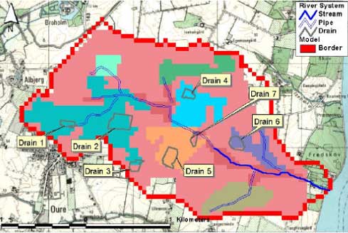
Figure 3.10 Stream system in Lillebæk. Different drain areas are connected – these are marked with different colours. Drain 1-7 are small drain areas, where drainflow is measured.
Figur 3.10 Å-system i Lillebæk. Forskellige drænede områder er tilsluttet å-systemet, disse er vist med forskellige farver. Dræn 1-7 er små områder hvor drænafstrømning er målt.
For Odder Bæk, it was not expected that drains would be of importance. However, the appearance of clay deposits near the soil surface indicates a need for artificial drainage in particular in the areas close to the stream. An effort was therefore made to identify existing drainage systems. At present, 25 -30 known drainage systems have been identified, most of which are located in the area around Riskær and along the piped runoff from Gislum Enge. It is, however, most likely that more drainage systems are active, but as these have been established long time ago by the local farmers advisory service, data are only accessible if the name of the farmer owning the land at the time of establishment is known. At present it is therefore assumed in the model that all areas near the stream are artificially drained. The depth of the drains is 1 m.
Within Odder Bæk catchment, one drain station has been monitored with respect to water flow and solute transport. It was therefore assumed that these data could be used for detailed calibration of parts of the model. In addition, information of pesticide application on the fields assumed to feed the drain station has been obtained through interviews with farmers. These should have been used for a cause and effect analysis - how long time does it take from application to a pesticide is found in drain water. The drain is shown on Figure 3.11.
Unfortunately it appears that a much larger area than indicated on Figure 3.11 drain to station 51. In , the model has estimated the topographical catchment for the drain station. It shows that the water caught by the drained area stem from the green and red triangular areas to the west of stream. This has implications for the interpretation of pesticide findings in the drain water.
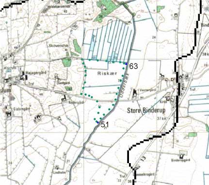
Figure 3.11 Location of the originally assumed drainage catchment and the drain station (51) in Odder bæk catchment. The assumed drainage area is delineated by the spots.
Figur 3.11 Placering af det forventede drænopland og drænstation (51) i Odder Bæk-oplandet. Drænoplandet er indrammet med prikker.
Model simulations based on the illustrated catchment area for the drain gave reasonable results during the winter season, but underestimated the flow during the summer season. This was not in accordance with the fact that groundwater measurements showed a falling water level during summer. The drainage system was investigated further and it became clear that side drains are found up to three meters from the stream at level with the bottom of the stream. Water may therefore, during the summer, move from the stream to the drain and back in the stream further down. Alternatively, there is an unidentified inflow from the north.
The conclusion is that the mass balance with respect to solutes on this drain is very doubtful and that the drain is not suited for validation of pesticide simulations.
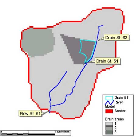
Figure 3.12 Drainage zones for different parts of the stream system. Note the estimated catchment for stream station 63 is the whole area upstream the station and the area for station 51 (dark gray) is larger than the actual pipe-drained area, indicated with a line.
Figur 3.12 Drænzoner for forskellige dele af å-systemet. Bemærk at det estimerede opland for å-station 63 er hele arealet opstrøms for stationen, og arealet til station 51 (mørkegrå) er større end det rør-drænede område, der er indikeret med en linie.
3.1.8 Abstraction
For Lillebæk, abstraction data from the County of Funen has been applied for the waterworks of Oure. On average, the yearly abstraction is approximately 100000 m3 influencing the overall water balance of the Lillebæk catchment significantly. Other individual water abstractions are present in the area, but none of them exceeds 3000 m3/year, which is found to be of local interest only.
In Figure 3.13 the four production wells of the waterworks of Oure are shown. It is seen that the screen of three of the wells is located in the lower primary aquifer whereas the screen of the last well is located in the upper secondary aquifer. During 1999-2000 BAM contamination has been monitored in two of the wells in the primary aquifer.
Figur 3.13 Vandforsyningsboringer tilhørende Oure vandværk. Filtersætningen i brøndene er vist med blå og vandspejlet med de trekantede markører.
Abstraction data were received from the county of Northern Jutland. Figure 3.14 shows the location of the wells. The total amount extracted from the Gislum Waterworks is constantly about 6.000 m3 per year, while extraction for irrigation differs from year to year – from almost nothing in year 1999 to 18.500 m3 in year 1992.
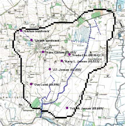
Figure 3.14 Water supply wells and irrigation wells located in the Odder Bæk catchment.
Figur 3.14 Placeringen af vandforsyningsbrønde og vandingsbrønde i Odder Bæk-oplandet.
3.2 Modelling water flow in the stream models
3.2.1 Cross-sections
The spatial discretion of the stream model is based on a series of cross-sections. Linear interpolation was conducted between these to define the calculation unit of the MIKE 11 model. To obtain an updated and detailed description of the geometry of the streams, measurement of the cross- sections conducted in the winter of year 1999 to 2000. The measured cross- sections were combined with existing information of cross-sections of the counties and a final cross section-data base was established for each set up of MIKE 11. The distance between the cross-sections depends on the uniformity of the stream and on the logistic constraints, such as the impossibility of measuring cross-sections in the dense forest of the catchment of Lillebæk. Hence the distance between the cross-sections varies between hundreds of meters at the most uniform sections of Odder Bæk to a few meters around bridges or other structures causing major local changes of the shape of the streams. An overview of the horizontal placement of the cross-sections in Lillebæk and Odder Bæk appear from Figure 3.15 and Figure 3.16 respectively, whereas the code of the bottom of the creek of each cross-section appears from Figure 3.17 and Figure 3.18 respectively.
Figure 3.15 Horizontal distribution of the cross-sections of the MIKE 11 model in the Lillebæk catchment
Figur 3.15 Horizontal fordeling af tværsnit i MIKE 11-modellen for Lillebæk-oplandet.
Figure 3.16 Horizontal distribution of the cross-sections of the MIKE 11 model in the Odder bæk catchment
Figur 3.16 Horizontal fordeling af tværsnit i MIKE 11-modellen for Odder Bæk-oplandet.
Figure 3.17 Altitude of the cross-sections of the MIKE 11 model in the Lillebæk catchment.
Figur 3.17 Kote for de i MIKE 11-modellen anvendte tværsnit fra Lillebæk-oplandet.
Figure 3.18 Altitude of the cross-sections of the MIKE 11 model in the Odder bæk catchment.
Figur 3.18 Kote for de i MIKE 11-modellen anvendte tværsnit fra Odder Bæk-oplandet.
3.3 Pesticide model for the catchment
3.3.1 Spraying data
The counties of Funen and Northern Jutland supplied GIS-maps with field numbers for 1998-2000, with corresponding files of management practices and pesticide use. These files contain information regarding date of spraying and amount sprayed. The information for selected pesticides is transformed to input for MIKE SHE. The overall use of pesticide in Lillebæk and Odder Bæk is shown in Table 3.3 and Table 3.4.
Table 3.3 Area treated with selected pesticides in Lillebæk from 1998 to 2000. Note that the spraying season of 1998 starts during autumn 1997.
Tabel 3.3 Areal behandlet med udvalgte pesticider i Lillebæk fra 1998 til 2000. Bemærk at sprøjtesæsonen 1998 begynder i efteråret 1997.
| 1998 | 1999 | 2000 | ||||
| Pesticide | ha | kg | ha | Kg | ha | kg |
| Bentazon | 17 | 3.7 | 7 | 2.2 | 6 | 4.2 |
| Pendimethalin | 148 | 57.8 | 24 | 9.5 | 267 | 135.6 |
| Fenpropimorph | 542 | 62.3 | 264 | 30.0 | 200 | 20.1 |
| Ioxynil | 165 | 12.9 | 248 | 18.6 | 190 | 13.7 |
| Ethofumesat | 31 | 3.4 | 35 | 3.9 | 56 | 6.3 |
| Isoproturon | 167 | 115.9 | 10 | 3.6 | 183 | 127.8 |
| Terbutylazin | 19 | 6.4 | 9 | 5.9 | 8 | 6.1 |
| Diuron | 2 | 1.2 | 1 | 1.0 | 16 | 16.9 |
| Pirimicarb | 116 | 7.5 | 93 | 8.9 | 98 | 6.7 |
| Prochloraz | 0 | 0.0 | 4 | 0.2 | 0 | 0.0 |
| Propiconazol | 456 | 17.8 | 233 | 9.2 | 109 | 4.5 |
* The sprayed area inside the catchment is only approximately 10 ha, as parts of the fields are outside the catchment. aTreated area overestimated as some of the fields included in the calculation are not located within the model catchment area. As a result of this the amounts may not represent exactly what is being applied within the model catchment.
Table 3.4 Area treated with selected pesticides in Odder Bæk from 1998 to 2000. Note that the spraying season of 1998 starts during autumn 1997.
Tabel 3.4 Areal behandlet med udvalgte pesticider i Odder Bæk fra 1998-2000. Bemærk at sprøjtesæsonen 1998 begynder i efteråret 1997.
| 1998 | 1999 | 2000 | ||||
| Pesticide | Ha | kg | ha | kg | ha | kg |
| Bentazon | 125 | 42.0 | 127 | 28.7 | 119 | 35.4 |
| Ethofumesat | 134 | 11.5 | 201 | 20.2 | 83 | 9.0 |
| Fenpropimorph | 185 | 24.3 | 245 | 27.4 | 224 | 24.4 |
| Ioxynil | 165 | 11.9 | 256 | 20.1 | 279 | 19.1 |
| Isoproturon | 94 | 44.1 | 116 | 53.7 | 116 | 25.0 |
| Pendimethalin | 165 | 97.5 | 222 | 102.2 | 213 | 114.0 |
| Terbutylazin | 61 | 29.9 | 72 | 23.0 | 10 | 2.6 |
| Diuron | 0 | 0.0 | 0 | 0.0 | 0 | 0.0 |
| Pirimicarb | 47 | 5.7 | 21 | 2.1 | 0 | 0.0 |
| Prochloraz | 21 | 0.5 | 0 | 0.0 | 21 | 4.8 |
| Propiconazol | 160 | 7.3 | 217 | 8.7 | 229 | 7.6 |
a Treated area overestimated as some of the fields included in the calculation are not located within the model catchment area. As a result of this the amounts may not represent exactly what is being applied within the model catchment.
3.3.2 Pesticide properties
The properties of the pesticides to be used for the simulation were extracted from the PATE database of the Danish Environmental Protection Agency. The treatment of the data turned out to be rather difficult as much of the data did not contain all the necessary information to transform the values to reference conditions. As part of the supporting information is confidential, the detailed calculations cannot be shown for most of the pesticides. However, the method used for normalisation of degradation values followed the guidelines given in FOCUS 2000.
The values used for modelling are given in Table 3.5.
Table 3.5 Pesticide properties extracted from the PATE database (Danish Environmental Protection Agency). The values (Halflife (DT50), sorption coefficient (Koc) and the Freundlich Exponent (1/n) are aggregated and normalised as described in FOCUS (2000). Not all data in the database could be normalised due to lack of information, and is therefore not included in the estimates.
Tabel 3.5 Pesticidegenskaber udtrukket af PATE-databasen (Miljøstyrelsen). Værdierne (Halveringstid (DT50), sorptionskoefficient (Koc) og Freundlich-eksponenten (1/n) er aggregeret og normaliseret som beskrevet i FOCUS (2000). Ikke alle data i databasen kunne normaliseres på grund af manglende information, disse er ikke inkluderet i estimaterne.
| Pesticide | DT50*, days | KOC ** | 1/n | Comments |
| Bentazon | 25.2 | 19.6 | both linear and freundlich adsorption among the results | |
| Pendimethalin | 66.3 | 15615 | 0.9¤ | It is stated in he data that adsorption follows a Freundlich isotherm, but no exponent is given. Degradation data results in a change in rate of 1.66 per 10 degrees (beta =0.0505) |
| Fenpropimorph | 22 | 4384 | Limited information, particularly on degradation | |
| Ioxynil | 1.86 | 236 | ||
| Ethofumesat | (45)& | 82.8 | The degradation data cannot be recalculated to reference conditions. | |
| Prochloraz | not collected | |||
| Isoproturon | 16.1# | 125 | 0.9¤ | It is stated in he data that adsorption follows a Freundlich isotherm, but no exponent is given. |
| Terbutylazin | 78.2 | 250 | 0.91¤ | A Q10-value of 3.43 was calculated from the values in the database. |
* The halflife is normalised to pF 2 and 20 degrees.
** For the freundlich values, KOC is determined at a concentration of 1 mg/l.
¤ In Odder Bæk, linear sorption was employed.
# Only two soils were included in the estimate from the PATE database. The dataset was extended with one soil from Lindhardt (1997). The extreme value was selected.
& No figure ws available for in the PATE database for DT50. A figure from the inception report (DHI et al., 1998) has been used.
3.3.3 Organic matter
In principle, the organic matter content of each of the known soil horizons should be used as input to the model. This is done in Lillebæk. However, for Odder Bæk, the soil types were modified compared to the original data, and no data existed for the organic soil. The values deduced are given in Annex B for each soil in the two catchments. Kd is then calculated as fOC * KOC. For Odder Bæk the foc-value are rather high and during the calibration phase, all values were halved in order to arrive at reasonable correspondence with observations.
3.3.4 Standard values
The default values for the FOCUS (2000) report were used for the following parameters as a starting point:
- The diffusion coefficient in water is 4.3 x 10⁻⁵ m2/day. This value is generally valid for molecules with a molecular mass of 200-250.
- Dispersion length is set to 5 cm.
- If nothing else is known, the Q10-factor is 2.2 (change in degradation rate with 10 degrees change in temperature).
- The exponent of the Walker equation, relating the degradation to soil moisture (f = (θ/θref)B, Walker, 1974), is 0.7.
- The degradation depth is supposed to decrease with depth. From 30-60 cm, the value is multiplied with 0.5 and from 60-100 cm with 0.3. Below 100 cm, no degradation is expected to take place. This assumption, however, turned out to be too conservative compared to observations and the factor of 0.3 was extended downwards into the upper part of the groundwater.
- If no data are available, and a Freundlich relation is expected, the default value for the exponent is 0.9. However, data available in the Pate database with the EPA only in one case supported the use of a Freundlich exponent. In addition, the concentration range in which these values are established is different from the concentration range found in at least the lower part of the soil profile.
- The transpiration stream concentration factor is set to 0 for non-systemic compounds and to 0.5 for systemic compounds.
- The interception factor by leaves is estimated on the basis of the plant cover at the time of spraying. The basic curves used to estimate this are shown in Styczen et al. (2004b, Appendix 2). The values stem from Jensen and Spliid (2003) or FOCUS (2000), depending on crop.
3.4 Pesticide model for streams and ponds
3.4.1 Solar insolation
To describe the photolytic degradation of pesticides, measurements of intensity (global radiation) and the spectral composition of the solar insulation is required. The global radiation data used was measured data for Hornum (st. no. 20501), which was considered to be representative for normal Danish conditions. The composition of the solar insulation was calculated from data given in OECD (1995). Average values for the four seasons (spring, summer, autumn, winter) are used.
3.4.2 Dispersion
For Lillebæk and Odder Bæk a constant dispersion coefficient of 3 m2s-1, typical of small Danish streams, was used (DHI, 1997).
3.4.3 Suspended matter, temperature and pH
Measurements of the temperature and pH from Lillebæk and Odder Bæk was obtained from the councils of Funen and North Jutland respectively. For pH the average values of 7.6 for the years of 1995 to 2000 was used. For temperature time series of daily measurements conducted at daytime between 10 am to 2 pm were used. In Lillebæk the measurements was conducted at Fredskovvej, whereas the measurement at Odder Bæk was conducted at station 61 at the Farsø Bridge.
Suspended matter was added to the stream model (MIKE11) from the catchment model as the flow of particles through macropores.
3.4.4 Biomass of macrophytes
Ideally, the biomass of the macrophytes should have been background data for the set up of the model, but quantitative data for macrophytes was not available for any of the streams. The biomass of macrophytes was therefore estimated on the basis of information from the literature (Jensen and Lindegaard 1996) of the yearly succession in the biomass of macrophytes in Danish streams not covered by forest Figure 3.19.
Figure 3.19 Biomass of macrophytes in light open danish streams.
Figur 3.19 Biomasse af makrofyter i lys-åbne Danske vandløb.
Based on the biomass of macrophytes was calculated assuming a forest cover of 50% for Lillebæk and 0% for Odder Bæk and an average depth of 0.1 m and 0.5 m for Lillebæk and Odder Bæk respectively.
3.4.5 Sediment bed
The diffusion into the sediment bed is heavily dependent on the size of the effective diffusion coefficient (Mogensen et al., 2004). On the basis of the calibration of the pond model against data for the experiments with artificial ponds (Helweg et al., 2003) an effective diffusion coefficient is determined and used for the sediment bed in ponds. For the stream a diffusion coefficient of 1.8 x 10⁻⁶ m2 h-1 corresponding to the molecular diffusion coefficient for a compound of a weight of 300 g mol-1 (Schwarzenbach, 1993) was used.
3.4.6 Sorption to sediment and suspended matter
For the compounds of Ioxynil, Bentazon and Pendimetelin, Kd, Koc, sorption and desorption rates were delivered by sub project 5 (Helweg et al., 2003). For the remaining compounds desorption rates was calculated from the Kd value as described in (Styczen et al., 2004b). Hence it is assumed that the ratio between the sorption and desorption rates is given by the Kd value and that sorption rate is compound independent and therefore similar to the sorption rate estimated for the above compounds. The validity of this assumption is further discussed by (Styczen et al., 2004b).
In case a Kd value was unavailable a Kd value was calculate either from the Koc or a Kow value for the pesticide and the organic content of the sediment/suspended matter as described by Styczen et al. (2004c). In every case the Kd, Koc or Kow values were extracted from a database, PATE, containing the data available for the EPA in connection with an approval procedure.
3.4.7 Sorption to macrophytes
Data for sorption to macrophytes are not available from the data delivered to the Danish EPA in connection with an approval procedure or from the PATE data base. The Kd values was therefore determined from the water solubility using adapted from Crum et al., (2000):
log(Kd) = 3.2 – 0.65 log(S), (Eq. 3.1)
where
S denotes the water solubility (mg/l).
Subsequently the kinetic of the sorption was determined from the Kd value as described for the sorption to particles (section 3.4.6).
3.4.8 Biological degradation in pore water and water column
On the basis of the biodegradation and sorption experiments of Helweg et al. (2003) a relative microbial activity of the free living bacteria and of the bacteria attacked to particles was calculated. Thereafter a total degradation rate and the particle concentration at which the degradation rate was determined were extracted from the data base PATE and the degradation rates of the dissolved pesticide in the pore water and in the water column was calculated as described by (Helweg et al., 2003).
3.4.9 Biological degradation at macrophytes
Data for biodegradation on macrophytes is not available from the data available to the EPA in connection with an approval procedure. In addition an approach for calculation of the biodegradation on macrophytes is not available from the literature. It was therefore decided not to include degradation on macrophytes in the model. The implication thereof is considered in the discussion.
Version 1.0 November 2004, © Danish Environmental Protection Agency