Calibration of Models Describing Pesticide Fate and Transport in Lillebæk and Odder Bæk Catchment
4 Calibration and Validation of Water Flow
Calibration is performed in a number of steps – one concerning the water flow and one concerning the pesticide transport. Calibration of the water flow was done stepwise too – on the stream flow, on the groundwater flow and on the drain flow separately, and on the integrated system.
4.1 Data for calibration
For calibration of the water flow, the main sources of information are drain runoff, stream runoff and groundwater levels measured in the two catchments. For calibration of the pesticide transport, the main source of information is concentrations measured at drain stations.
As mentioned in Section 1.1, stream flow is measured at two stations, drain flow at 6 stations and head elevation at 15 wells in Lillebæk. Pesticide is measured at drain 2 and 6, and at the two flow stations (see Figure 4.1). The locations of the observation wells have during the calibration been a somewhat uncertain. Latest locations are used in the report and calculation of calibration statistics – some of these updates are done on basis of re-measuring the locations using GPS.
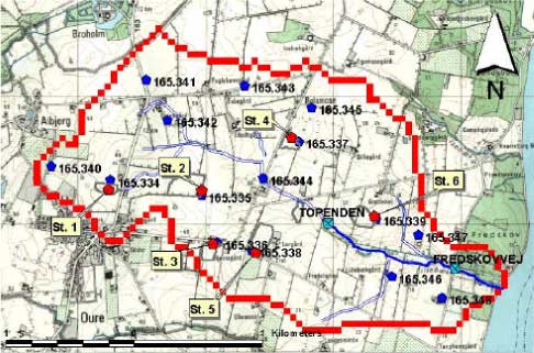
Figure 4.1 Location of measurement stations in Lillebæk - head elevation wells (blue petagons), flow measurement stations (crossed squares) and drainflow stations (St. 1-6).
Figure 4.1 Placering af målestationer i Lillebæk – pejleboringer (blå femkanter, afstrømningsmålere (firkanter med kryds) og drænafstrømnings-stationer (St. 1-6).
In Odder Bæk, stream flow is also measured at 3 stations, drain flow at one station and head elevation is measured in 17 groundwater wells, see Figure 4.2. The intermediate flow station was only active for at few years. Pesticide is measured in drain 51 and at the downstream station.
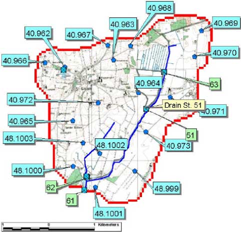
Figure 4.2 Location of measurements in Odder bæk - head elevation wells (blue petagons), flow measurement stations (crossed squares) and drainflow station (51).
Figur 4.2 Placering af målestationer i Odder Bæk – oplandet – pejleboringer (blå femkanter, afstrømningsmålere (firkanter med kryds) og drænafstrømningsstation (51).
Measurements of water generally cover the period from 1989 till 2000. Pesticide measurements were only carried out in 1999 and 2000 (end September).
The pesticide measurements are described by Iversen et al. (2003).
4.2 Calibration of water flow
4.2.1 Initial calibration of the MIKE 11 HD model
Before integration of the stream model (MIKE 11) into the catchment model, calibrations of the hydraulics was conducted. Calibration was performed for the period between 1989 to 1998. Measurements of discharge and water levels were use in the calibration. To take into account the water that enters the streams from the sides the difference between the water flow at the upstream and down stream stations was calculated and added as separate sources distributed evenly along the course of the streams.
For Lillebæk data from the stream stations shown on Figure 4.1 was used – i.e. discharge at the stream station at Fredskovvej and Topenden, and calibration was done on the water level at Fredskovvej.
For Odder Bæk, a similar calibration was conducted on the basis of measurements of discharge at stream station 61 and 63 and water levels at the stream station 61, see Figure 4.2.
4.2.2 Calibration of the MIKE SHE model
A proposed procedure for calibration/validation was described in the first status report of the project (DHI et al., 2000e). This procedure has been followed. However, soil moisture data were not used in the calibration.
Calibration was carried out as a split-sample – using part of the period for actual calibration and part of the period for validation. The actual calibration was done using trial and error procedure where each calibration simulation has been evaluated by statistical measures (mean error and root mean square). Calibration has been performed on different scales – mainly on catchment scale but also on drain catchment scale and single column scale.
On catchment scale the main parameters subject to calibration have mainly been the conductivities in the saturated zone, the leakage coefficient between the stream and the groundwater, and the drainage coefficient. The drainage coefficient is one of the main processes in both areas, however described by the least physical parameters. Besides, the exact location of the drain is somewhat uncertain. The measured stream flow and the groundwater levels have been the targets for the calibration.
Also the depth of the drains has been subject to calibration. The target for these calibrations has been the measured drain outflow. Results from the drain studies have been applied to the catchment models.
Soil properties have been subject to very restricted calibration. The field data and corresponding parameter estimations have provided the limitations for the values tried. The effect of different crops and soil types has been examined using the groundwater level as target. Results from the soil column calibrations are very uncertain due to boundary effects. The results have been test on catchment scale before they were applied.
In addition, simulations with the Daisy model were performed to test the general transport parameters selected for the soil profile. The test substance was nitrate. This exercise is not reported in detail, as it is only indicative for the pesticide modelling, and because several N-related factors have to be parameterised, which are not relevant for pesticide modelling anyway. However, for Lillebæk, the simulated and modelled nitrate fluxes were in good correspondence, and the setup has been handed over to the county of Funen and NERI. For Odder Bæk, the exercise is less interesting as the soil profiles required modifications to be used in the catchment model, and they are thus not directly comparable.
4.2.2.1 Lillebæk
Simulated and measured flow for the two stream stations in Lillebæk is shown in Figure 4.3. The dynamics of the flow is considered well described, and the error of the overall water balance is 3% only at the downstream end.
Figure 4.3 Measured and simulated flow (m3/s) in the upstream and downstream stream station in Lillebæk catchment.
Figur 4.3 Målt og simuleret afstrømning (m3/s) i den opstrøms og nedstrøms målestation i Lillebæk-oplandet.
Figure 4.4 Measured and simulated accumulated flow in Lillebæk at the two stream stations.
Figur 4.4 Målt og simuleret akkumuleret afstrømning i Lillebæk ved de to afstrømningsmålestationer.
At the upstream station, the water balance error is 30%, mainly due to too much simulated flow during summer and additional discrepancy in 1995. Some of this uncertainty may be due to uncertainty regarding exactly where different drain systems are connected to the stream. Besides, the boundary conditions on the southern border in the sand lens are somewhat uncertain. Further field investigation is likely to reveal whether groundwater flow in the lens is towards the Hammersbro Bæk or Lillebæk – in other words, the location of the groundwater divide in the area influences the modelling.
Simulated and observed groundwater potentials in 15 wells is shown in Figure 4.5 - Figure 4.8. All values are related to the top layer – though it seems at little odd that the filter is placed in the clay rather than in the white sand layer.
In general there is at good match between the simulated and observed levels. In a majority of the wells there is a good match with the dynamics. Three wells are found to match neither the dynamics nor the level. Unfortunately these are all placed in the southern quadrant, see Figure 4.7. Modifications of the boundary conditions of the sand lens had good effect on calibration of these wells – however, with the given geological model it was not possible to lower the potential head on the boundary further.
Calibration on the period of 1989 to 1992 and the evaluation was done on statistical measures, mean error and root mean square error, standard deviation and Nash-Sutcliffe coefficient. The statistical measures are listed in Tabel 4.1, both for the calibration period the following validation and the total period 1989 to 2000.
For the groundwater level, the mean error, the root mean square error and the standard deviation on the residuals were used – using the equations listed below, where the following symbols are used:
Oi = Value of observation no. i
Pi = Value of prediction no. i
N = Number of observations
Mean error
![]()
Root mean square error
![]()
Standard deviation
![]()
For the river flow the evaluation measures used are the mean error, the root mean square error and the Nash-Sutcliffe coefficient. This coefficient investigates whether it is better to look at the average value of the measurements than at the model predictions. The interval of NS is ]-∞;1].
Nash-Sutcliffe coefficient
Table 4.1 Statistical measures on match between observed and simulated flow and groundwater level in Lillebæk. Values for calibration, validation and total period.
Tabel 4.1 Statistiske mål på overensstemmelsen mellem observeret og simuleret afstrømning og grundvandsniveau i Lillebæk. Værdier for kalibreringen, valideringen og den totale periode.
| Obs. ID | Calibration 1989-1992 | Validation 1993-2000 | Whole 1989-2000 | ||||||
| ME [m3/s] |
RMSE [m3/s] |
NS [-] |
ME [m3/s] |
RMSE [m3/s] |
NS [-] |
ME [m3/s] |
RMSE [m3/s] |
NS [-] |
|
| Fredskov | -0.0003 | 0.0210 | 0.7091 | -0.0022 | 0.0302 | 0.7128 | -0.0018 | 0.0273 | 0.7124 |
| Topenden | -0.0029 | 0.0118 | 0.7449 | -0.0057 | 0.0171 | 0.7171 | -0.0048 | 0.0154 | 0.7258 |
| Average | -0.0016 | 0.0164 | 0.7270 | -0.0040 | 0.0237 | 0.7150 | -0.0033 | 0.0214 | 0.7191 |
| ME [m] |
RMSE [m] |
STD [m] |
ME [m] |
RMSE [m] |
STD [m] |
ME [m] |
RMSE [m] |
STD [m] |
|
| 165.334 | 0.62 | 0.84 | 0.58 | 0.39 | 1.01 | 0.93 | 0.40 | 1.00 | 0.92 |
| 165.335 | 0.74 | 0.82 | 0.34 | 0.35 | 0.56 | 0.44 | 0.36 | 0.57 | 0.45 |
| 165.336 | -1.44 | 1.47 | 0.30 | -1.36 | 1.63 | 0.90 | -1.36 | 1.63 | 0.88 |
| 165.337 | 1.01 | 1.35 | 0.90 | 0.66 | 1.07 | 0.84 | 0.67 | 1.08 | 0.85 |
| 165.338 | -5.04 | 5.26 | 1.51 | -5.06 | 5.18 | 1.11 | -5.06 | 5.18 | 1.13 |
| 165.339 | -0.69 | 0.79 | 0.37 | -1.06 | 1.10 | 0.29 | -1.04 | 1.09 | 0.30 |
| 165.340 | 2.60 | 2.66 | 0.57 | 2.31 | 2.47 | 0.87 | 2.42 | 2.55 | 0.78 |
| 165.341 | 0.70 | 0.89 | 0.54 | 0.64 | 1.15 | 0.96 | 0.66 | 1.07 | 0.84 |
| 165.342 | -0.25 | 0.60 | 0.55 | -0.52 | 0.95 | 0.80 | -0.41 | 0.83 | 0.72 |
| 165.343 | -0.21 | 0.35 | 0.28 | -0.10 | 0.45 | 0.44 | -0.14 | 0.41 | 0.38 |
| 165.344 | -2.40 | 2.45 | 0.52 | -2.71 | 2.79 | 0.66 | -2.55 | 2.63 | 0.61 |
| 165.345 | 1.55 | 1.73 | 0.77 | 1.45 | 1.63 | 0.74 | 1.49 | 1.67 | 0.76 |
| 165.346 | -0.22 | 0.29 | 0.20 | -0.45 | 0.62 | 0.43 | -0.36 | 0.51 | 0.37 |
| 165.347 | -0.37 | 0.42 | 0.19 | -0.54 | 0.60 | 0.26 | -0.47 | 0.53 | 0.25 |
| 165.348 | -1.19 | 1.22 | 0.27 | -0.87 | 1.18 | 0.79 | -0.99 | 1.19 | 0.67 |
| Average | -0.31 | 1.41 | 0.53 | -0.46 | 1.49 | 0.70 | -0.43 | 1.46 | 0.66 |
Is that excellent, good or just acceptable? Early in the project an attempt was made to set limits for this (reported in DHI et al., 2000e). However, the limits were set on a rather arbitrary basis. Recently a guide to groundwater modelling has been published in Danish (Ståbi i grundvandsmodellering, GEUS, Henriksen et al. (red) (2000)), also considering issues on performance criteria. For the groundwater level, criterions are depending on the overall difference in measured groundwater table throughout the area – 5% for the ME and 10% for the RMSE for an excellent model.
Having a groundwater level in the area between 8 and 50 meters the criterion is 2.1 meter and 4.2 meter to the ME and RMSE, respectively. On the average this is clearly fulfilled, and only a few wells do not meet the demands.
For the river flow the criterion is less clear – however from examples in the guide the criterion were that if the median flow is less than 0.05 m3/s the deviation can be set to 100% on the ME and 200% on the RMSE. These values give a criterion of 0.03 m3/s on the ME and 0.06 m3/s on the RMSE – the model meets both.
The standard deviation and the Nash-Sutcliffe are not considered in the guide to groundwater modelling – however, some limits were suggested in DHI e al., 2000e.
For the standard deviation on the groundwater level residuals the criterion to an excellent, good or acceptable model in status report 1 is – 0.25 m, 0.40 m and 0.50 m respectively. None of these are meet on the average and only a few wells meet the criterion of an excellent model. It is clear, however, that the criteria are considerably stricter than what is specified in the Danish guidelines, and probably unrealistic.
For the Nash-Sutcliffe coefficient for the river flow the criterion is – 0.9, 0.8 and 0.7 for an excellent, good and acceptable model respectively. The Nash-Sutcliffe coefficient was in status report called R2 – here it is named NS (see Table 4.1). Here the model ranges as acceptable.
The conclusion is that compared to the recent groundwater modelling guide, the model ranges as excellent, while compared to the very ambitious (and probably unrealistic) goals set earlier in the project, the model only just reaches acceptable.
Figure 4.5 Measured and simulated groundwater potential in wells located in the northern quadrant of the Lillebæk catchment. The location of the wells are shown in Figure 4.1.
Figur 4.5 Målt og simuleret grundvandspotentiale i brønde i den nordlige kvadrant af Lillebæk-oplandet. Brøndenes placering er vist i Figur 4.1.
Figure 4.6 Measured and simulated groundwater potential in wells located in the eastern quadrant of the Lillebæk catchment. The location of the wells are shown in Figure 4.1.
Figur 4.6 Målt og simuleret grundvandspotentiale i brønde i den østlige kvadrant af Lillebæk-oplandet. Brøndenes placering er vist i Figur 4.1.
Figure 4.7 Measured and simulated groundwater potential in wells located in the southern quadrant of the Lillebæk catchment. The location of the wells are shown in Figure 4.1.
Figur 4.7 Målt og simuleret grundvandspotentiale i brønde i den sydlige kvadrant af Lillebæk-oplandet. Brøndenes placering er vist i Figur 4.1.
Figure 4.8 Measured and simulated groundwater potential in wells located in the western quadrant of the Lillebæk catchment. The location of the wells are shown in Figure 4.1.
Figur 4.8 Målt og simuleret grundvandspotentiale i brønde i den vestlige kvadrant af Lillebæk-oplandet. Brøndenes placering er vist i Figur 4.1.
4.2.2.2 Odder Bæk
Simulated and measured flow for the upstream, downstream station, and the drain in Odder Bæk is shown in Figure 4.9. The average error on the downstream flow is 5% and 13% on the upstream flow. It is obvious, however, that the drain flow is poorly simulated during the summer period. As described in section 1.1.5, the catchment for the drain is much larger than anticipated at the start of the project. Furthermore, the drain is found in the same depth as the bottom of the stream and only 3 meters from the stream. The only explanation of the water in the drain during the summer is that water runs from the stream to the drain, as the groundwater is found at greater depth. The drain is therefore not suitable for pesticide calibration.
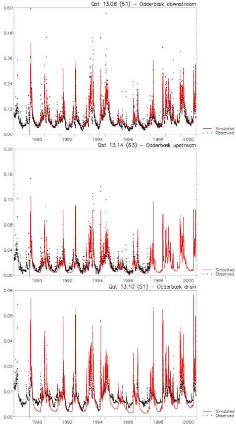
Figure 4.9 Measured and simulated flow (m3/s)at the downstream, at the upstream and at the drain station in Odder Bæk.
Figur 4.9 Målt og simuleret afstrømning (m3/s) ved den nedstrøms og den opstrøms afstrømningsstation og drænstationen i Odder Bæk.
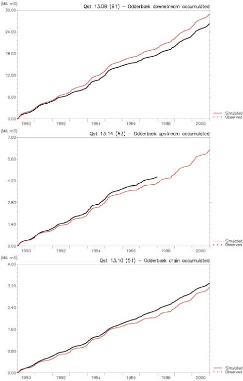
Figure 4.10 Measured and simulated accumulated flow at the downstream, at the upstream and at the drain station in Odder Bæk.
Figur 4.10 Målt og simuleret akkumuleret afstrømning ved den nedstrøms og opstrøms afstrømningsstation og drænstationen i Odder Bæk.
Simulated and observed groundwater potentials in 17 wells is shown in Figure 4.11. Values are related to the layer covering the filter.
In general the match between the simulated and observed levels is fair. In 11 of the well there is found a fair match on the dynamics. In 5 (40.962, 40.967, 40.968, 48.1000 and 48.999) out of the 11 wells the level is matched too – those wells are located in the northern and southern part of the model area. The most southern well (48.1001) is very close to the border – and here neither the dynamics nor the level is matched. The observations are placed above the applied surface topography. Also in the well between Odder Bæk and Gislum Enge the observations is found to be above the surface topography. In the eastern part the observations are matched on the levels but not on the dynamics.
Table 4.2 Statistical measures on match between observed and simulated flow and groundwater level in Odder Bæk. Values for calibration , validation and total period.
Tabel 4.2 Statistiske mål for overensstemmelsen mellem observeret og simuleret afstrømning og grundvandsniveau i Odder Bæk. Værdier er givet for kalibreringen, valideringen og den totale periode.
| Obs. ID | Calibration 1994-1996 | Validation 1996-2000 | Whole 1990-2000 | ||||||
| ME [m3/s] |
RMS [m3/s] |
NS [-] |
ME [m3/s] |
RMS [m3/s] |
NS [-] |
ME [m3/s] |
RMS [m3/s] |
NS [-] |
|
| Downstream | -0.0026 | 0.0417 | 0.63 | -0.0048 | 0.0361 | 0.45 | -0.0040 | 0.0394 | 0.51 |
| Upstream | 0.0022 | 0.0119 | 0.54 | 0.0030 | 0.0078 | 0.26 | 0.0023 | 0.0112 | 0.42 |
| Drain | 0.0068 | 0.0081 | -1.36 | 0.0063 | 0.0069 | -2.94 | 0.0066 | 0.0076 | -1.73 |
| Average | 0.0021 | 0.0206 | -0.06 | 0.0015 | 0.0169 | -0.74 | 0.0016 | 0.0194 | -0.27 |
| ME [m] |
RMS [m] |
STD [M] |
ME [m] |
RMS [m] |
STD [M] |
ME [m] |
RMS [m] |
STD [M] |
|
| 40.962 | -1.56 | 1.58 | 0.27 | -1.13 | 1.13 | 0.14 | -1.30 | 1.33 | 0.29 |
| 40.963 | -0.96 | 0.99 | 0.22 | -0.78 | 0.80 | 0.18 | -0.85 | 0.88 | 0.22 |
| 40.964 | -2.00 | 2.01 | 0.22 | -1.92 | 1.92 | 0.19 | -1.96 | 1.97 | 0.20 |
| 40.965 | -3.00 | 3.01 | 0.22 | -3.00 | 3.02 | 0.32 | -3.00 | 3.01 | 0.27 |
| 40.966 | 1.23 | 1.28 | 0.36 | no obs. | no obs. | no obs. | 1.23 | 1.28 | 0.36 |
| 40.967 | -0.05 | 0.16 | 0.15 | no obs. | no obs. | no obs. | -0.05 | 0.16 | 0.15 |
| 40.968 | 0.03 | 0.10 | 0.10 | 1.72 | 1.72 | 0.04 | 0.69 | 1.07 | 0.83 |
| 40.969 | 1.04 | 1.71 | 1.36 | no obs. | no obs. | no obs. | 1.04 | 1.71 | 1.36 |
| 40.970 | 0.15 | 0.50 | 0.47 | no obs. | no obs. | no obs. | 0.15 | 0.50 | 0.47 |
| 40.971 | -0.21 | 0.47 | 0.42 | no obs. | no obs. | no obs. | -0.21 | 0.47 | 0.42 |
| 40.972 | -2.02 | 2.05 | 0.38 | no obs. | no obs. | no obs. | -2.02 | 2.05 | 0.38 |
| 40.973 | 0.41 | 0.94 | 0.84 | no obs. | no obs. | no obs. | 0.41 | 0.94 | 0.84 |
| 48.999 | 0.15 | 0.35 | 0.32 | 0.26 | 0.37 | 0.26 | 0.23 | 0.37 | 0.30 |
| 48.1000 | 0.43 | 0.49 | 0.23 | 0.41 | 0.44 | 0.17 | 0.41 | 0.45 | 0.20 |
| 48.1001 | 3.07 | 3.07 | 0.21 | no obs. | no obs. | no obs. | 3.07 | 3.07 | 0.21 |
| 48.1002 | 2.07 | 2.09 | 0.27 | no obs. | no obs. | no obs. | 2.07 | 2.09 | 0.27 |
| 48.1003 | 0.20 | 0.35 | 0.29 | no obs. | no obs. | no obs. | 0.20 | 0.35 | 0.29 |
| Average | -0.06 | 1.24 | 0.37 | -0.64 | 1.34 | 0.18 | 0.01 | 1.28 | 0.42 |
The final calibration on the period of 1994 to 1996 and the evaluation of the model has been done using statistical measures, mean error and root mean square. The statistical measures are listed in Table 4.2, both for the calibration period, the following validation and the total period 1990 to 2000.
Using the guidelines – mentioned under the Lillebæk calibration – for setting the criterion to the ME, RMSE and STD for the groundwater level an excellent model fulfils the 1.0 m, 2.0 m and 0.25 m for the three statistical measures. A measured groundwater level span in the area from the lowest 15 meter to the highest 35 meter gives the criterion of 1 and 2 meters to the ME and RMSE, and the 0.25 m criterion to the STD is taken from DHI et al. (2000e).
The model complies with the performance criteria for an excellent model – except for the STD-criteria were the model can be characterised as a good model.
The average flow downstream is around 0.07 m3/s – between 0.05 and 0.1 m3/s. The recommended criterion is 50% and 100% – which gives a criterion to the ME and RMSE of 0.035 and 0.07 m3/s. The model meet these performance criteria.
For the STD the criterion taken from the 1st status report 0.7 for an acceptable model. Even disregarding the performance in the drain station will not give a model performance that can fulfil this criterion. The conclusion must be that the criteria set up earlier in the project were unrealistically strict.
Again the conclusion is that according to the guide on groundwater modelling, the model is excellent.
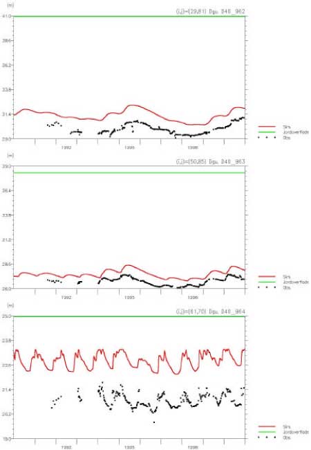
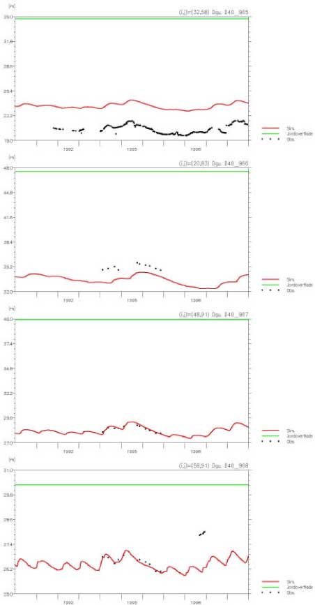
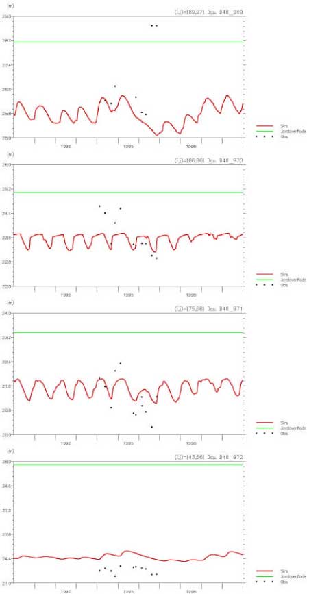
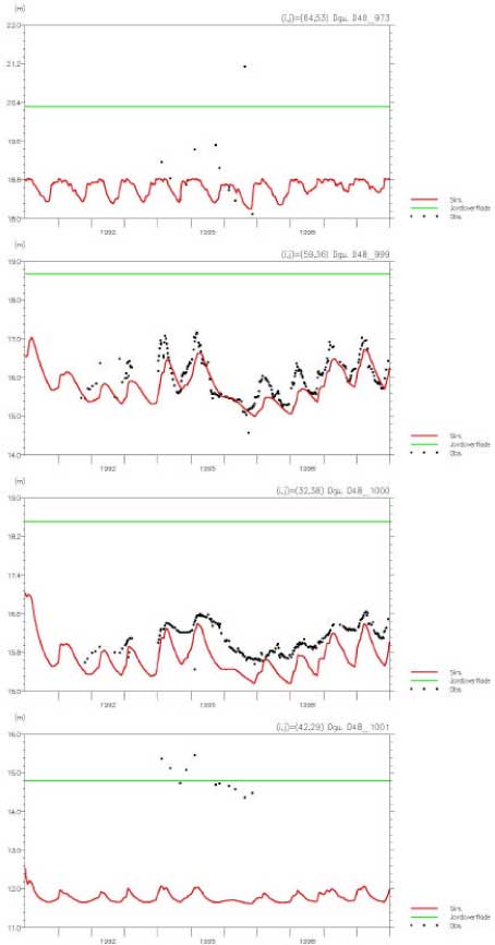
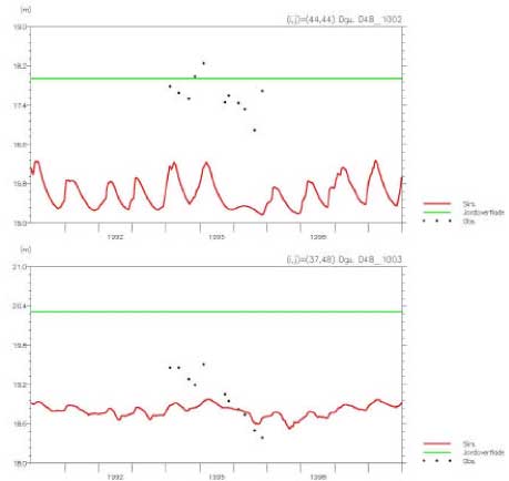
Figure 4.11 Measured and simulated groundwater potential in wells located in Odder bæk catchment.
Figur 4.11 Observeret og simuleret grundvandspotentiale i brønde i Odder Bæk-oplandet.
Version 1.0 November 2004, © Danish Environmental Protection Agency