|
Fate of Pyrethroids in Farmland Ponds 13 Model formulations, part II
The assumptions listed in the previous chapter will form the platform for the mathematical model formulation. Each sub-model will first be presented and subsequently they will be combined to form a series of possible mathematical models. 13.1 Formulation of sub-modelsThe models for the processes will first be described followed by the models for transport. The reason for this order is the fact that the transport models need the local process modelling in order to be complete. 13.1.1 Process modellingAdsorption The substance is assumed to be sorbed to different kinds of sorption medium in form of sediment solids, suspended solids in the water column or biota (macro phytes) or by other molecules in the surface micro layer. The sorption is assumed linear, reversible and instantaneous yielding an expression as (13.1)
where cs is the concentration (in relation to the dry mass of sorption medium) of sorbed substance (μg/kg), cd is dissolved substance concentration (μg/l) and Kd is the sorption coefficient (l/kg). A mass balance for the substance (13.2)
where ctot is the total concentration (μg/l), θ is the volume fraction of water, r is the dry bulk density of the sorption medium (kg/l). A combination of (13.3)
where R is defined as a retention factor. Degradation First order degradation is defined by the equation (13.4)
where Dgr is the rate of degradation (μg/(l h)) and k is the first order degradation coefficient (1/h). 13.1.2 Transport modellingVolatilisation Volatilisation is assumed to follow a first order relationship with respect to the dissolved water column concentration (13.5)
where vola is the volatilisation rate per surface area (μg/(m2 h)), kvol is the 1. order rate constant for volatilisation (l/(m2h)) and cd,wc is the concentration of dissolved substance in the water column (μg/l). Sedimentation The sedimentation rate of suspended solids in the water column to the bottom (sediment) is assumed constant and the adsorption to the solids is assumed linear, reversible and instantaneous, yielding (13.6)
where sed is the rate of removed substance per water column cross section area (μg/(m2 h), kdsus is the adsorption coefficient between the dissolved phase and the phase adsorbed to suspended solids in the water column (kg/l) and vsed is the sedimentation flux of suspended solids (kg/(m2h)) Diffusion The one dimensional equation for diffusion is derived using a mass balance for an infinitesimal control volume. The detailed derivation is done in a series of text books (f.ex. Crank, 1975) and is not repeated here. The diffusion equation combined with the equation for degradation (Eq. 13.4) (13.7)
where ctot and cd is the total and dissolved substance concentration (μg/m3) respectively at the actual place (e.g. in the sediment), D is the diffusion coefficient (m2/h), k is the degradation constant (1/h). Note: when the diffusion equation is used the volume unit for the concentration values is based on m3 instead of l in order to keep a fundamental unit for D (m2/h). This equation can be expressed in terms of only one concentration parameter using Eq. 13.3 to eliminate ctot (13.8)
where R is the retention factor. The values for D, R and k are assumed constant in time and space according to the assumption listed in chapter 12.2. The initial and boundary conditions will be presented at the specific model presentations. 13.2 Combining the sub modelsThree main compartments The pond system consists of three main compartments of interest: (1) surface micro layer; (2) water column; (3) sediment. The main part of substances will typically be present in only one of these three places at a specific time. In the very beginning after spraying the main part of the substance is in the surface micro layer. In the next period the main part of the substance will typically be in the water column and finally the sediment may be the sink for the major part of the substance. The importance of the surface micro layer As seen in Figure 11.1, the highest concentration measured in the surface micro layer for low dosage (SML) is approximately 500 μg/l (fenpropathrin) and the thickness of the layer sampled is approximately 340 μm. If the total dosage in this case (5 mg/m2) is mixed into a 340 μm deepness, as sampled, the concentration will be 15000 μg/l. Thus, most of the substances (more than 95 %) is transported though the sampled layer already before the time for the first sampling. Even though the SML does not seem to be the place for the main fraction of the substance after 1 hour, the SML may still be important from an ecotoxicological view point. The SML will be presented separately from the water column and sediment models. The water column and sediment, on the other hand, have to be described together. Surface micro layer characteristics 13.2.1 Surface micro layer (SML)The substance is sprayed at the top of the surface as a layer of uniform thickness. After spraying the substance will diffuse though the SML by molecular diffusion and be released to the water column below the SML. Adsorption is assumed to take place to an immobile phase which could be any kind of organic macro molecules, which may adsorb the substance and which moves "much slower" by diffusion than the substance or it could be a surfactant attracted to the surface. The adsorption is assumed to be uniform in the SML and no degradation is assumed to take place. The surface micro layer model Based on the above the following equation develops from Eq 13.8 (13.9)
where cSMLd is the dissolved substance concentration ( μg/m3) in the SML, DSML and RSML are the diffusion coefficient (m2/h) and retention factor (-) respectively in the SML. The initial conditions are (13.10a)
where Ldosage is the thickness of the layer sprayed at the top of the SML during the application, t is the time since spraying (h) and x is the downward distance from the surface (m). The boundary conditions are (13.11a)
(13.11b)
where LSML is the thickness of the SML (m), and cd,wc is the dissolved substance concentration in the water column (μg/l). The volatilisation of the substances from the surface into the air is assumed to be of first order in relation to the concentration at the water/air interface. 13.2.2 Water column and sedimentPossible models A series of possible models are presented in this chapter and these models will be discussed relative to each other in the following model analysis. Each model has an identification number and the simulated mechanisms, in the following denoted elements, are summarised in Table 13.1. Table 13.1 Et overblik over de mekanismer, der indgår i de forskellige modeller.
Simulated mechanisms In Table 13.1 degradation, volatilisation and removal by sedimenting solids relate to the same element for the water column, because, it is not possible to separate them as long as they are described as a 1. order removal. The arguments for the chosen combination of elements are: (1) no more than two elements in each model in order not to make the models too complex; (2) a water column degradation or sediment transport element has to be included in order to assure a concentration decrease with time; (3) in the sediment, adsorption has to be included because of the hydrophobic nature of all the substances. The reason why there is no model solely for degradation in the water column is that the measured values are total values including suspended solids and dissolved phases and therefore it is impossible to distinguish between adsorption and no adsorption (a more detailed argumentation follows in the presentation of model 1). Model 1, Degradation and adsorption to suspended solids in the water column The following removal processes are considered: (1) degradation (Eq. 13.4), (2) volatilisation (Eq. 13.5) and (3) sedimentation of solids (Eq.13.6), combining all the equations in a mass balance yields (13.12)
where ctot,wc is the total concentration in the water column (μg/l) including both dissolved and adsorbed substance. Combining Eq. 13.12 and 13.3 gives (13.13)
where Rsus,wc is the retention factor for adsorption to suspended solids and keff is the effective removal constant for the total concentration. Rsus,wc is defined by Eq 13.3, where the volume fraction of water (θ) is close to unity and the dry bulk density (ρ) is the concentration of the adsorption medium. Eq. 13.13 shows how different processes can be combined to form a simple 1. order removal model. Assuming completely mixed conditions the initial conditions for Eq. (13.13) is (13.14)
where Lwc is the water depth. Model 2, 1. order removal in the water column including adsorption to the macrophytes This model is closely related to model 1 the only difference being the relationship to the measurements. The substance sampling includes both the dissolved phase and the phase adsorbed to suspended solids, while adsorption to macrophytes or other kind of macroscopic adsorption are not included. Therefore, in case of sorption to macrophytes the concentration measured is only the dissolved concentration and the model has to be derived in relation to the latter. Combining Eq. 13.12 and Eq. 13.3 gives (13.15)
where Rmacro,wc is the retention factor for macrophyte adsorption. Similar to Rsus,wc the Rmacro,wc parameter is defined by Eq. 13.3 the only difference to Rsus,wc being the dry bulk density (ρ), which in case of Rmacro,wc is related to larger, non dispeRsed media, e.g. macrophytes. Eq. 13.15 has the same form as Eq. 13.12, but the model is different because of different initial conditions. The initial condition for model 2 is (13.16)
Model 3, Transport and adsorption within the sediment In this model only transport (diffusion) and adsorption mechanisms in the sediment are considered neglecting degradation, which results in a reduced form of Eq. 13.8 as (13.17)
where cd,sed is the dissolved concentration in the sediment pore water, Dsed is the effective diffusion coefficient through the sediment pores (m2/h), Rsed is the retention factor in the sediment and x is the downward distance from sediment surface (m). The sediment concentration cd,sed is dependent on both time and space yielding a concentration profile at a given time, while the concentration in model 1 and model 2 depends only on the time progress. The initial condition for the sediment concentration is (13.18)
The boundary conditions at the sediment surface is derived using a mass balance for the water column assuming no adsorption and degradation in the water column ending up in the equations as (13.19a)
(13.19b)
(13.19c)
The diffusion term in Eq. 13.19a reflects the "suction" of substance from the water column into the sediment by diffusion. The pore water concentration value at the top of the sediment ( The downward boundary condition deep in the sediment is assumed to be an open boundary where the substance can be transported to an infinite depth (13.20)
This equation may becomes problematic if the model calculations predict a significant amount of the substance to be transported deep into the sediment. Because in that case the sediment properties may change dramatically and the assumption of homogenous sediment conditions will become invalid. Model 4, Adsorption to suspended solids in the water column and transport and adsorption within the sediment This model is equivalent to model 3 with regard to the sediment equations the only difference being the boundary conditions for the relationship between the water column and sediment. Only dissolved substance is transported into the sediment, so, the existence of adsorption to solids in the water column will affect the transport rate into the sediment. The effect of filtering fauna at the sediment surface is assumed to be negligible in this context. The set of equations in Eqs. 13.19a-c has to be reformulated to take into account the adsorption of substance in the water column. The mass balance for the water column needs to be expressed in terms of the total concentration (ctot,wc) including the mass of adsorbed substance. Taken this into account, Eqs. 13.19a-b are reformulated as (13.21a)
(13.21b)
(13.21C)
The model calculations relates to the measurements by comparing the values of ctot,cw because the sampling includes the substance adsorbed to the suspended solids. Model 5, Adsorption to macrophytes in the water column and transport into the sediment This model is similar to model 4 in all the calculations the only difference being the relationship between model simulations and measurements. Model 4 compare the values for ctot,cw to the measurements while model 5 compare cd,cw to the measurements because the substance adsorbed to the macrophytes are not included in the measurements. The retention factor in the water column is in relation to the macrophytes (Rmacro,wc) and not in relation to the suspended solids (Rsus,wc) as in model 4. Model 6, Degradation in the water column and transport and adsorption within the sediment The transportation in the sediment is calculated by neglecting the degradation in Eq. 13.8 (see, Eq. 13.17). The initial conditions for the sediment is given as in Eq. 13.18. The upper boundary conditions at the sediment surface is derived using a mass balance for the water column assuming no adsorption and 1. order degradation in the water column (13.22a)
(13.22b)
(13.22c)
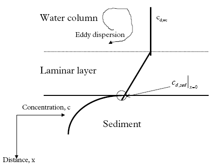
where keff is the effective degradation constant (1/h) which can involve more than just degradation as illustrated by Eq. 13.13. Model 7, Transport and adsorption within the sediment though a laminar boundary layer at the sediment/water column interface In this model a laminar layer of stagnant water is assumed to exist between the sediment and the water column. This layer is well established as a consequence of friction between the
bottom and the free water above. The transport through this layer which is diffusion controlled may be rate limiting if the sediment uptake is rapid. The only difference between model 7
and model 3 is the relationship between the dissolved concentration in the water column (cd,wc) and the dissolved sediment pore concentration at the sediment surface ( (13.23)
where Rate is the rate of transport per unit sediment area (μg/(m2h)), Dlayer is the diffusion coefficient in the layer (m2/h), and Llayer is the layer thickness (m). The concentrations cd,wc and cd,sed above and under the layer respectively are illustrated in Figure 13.1. The transport rate for passing the sediment surface by diffusion is given by (13.24)
An equation for the concentration at the sediment surface is derived by combining Eqs. 13.23 and 13.24 (13.25)
where Klayer is the effective layer transport resistance (m). If the diffusion coefficient is equivalent for the boundary layer and the sediment pore water, Klayer will simply be the layer thickness (Eq. 13.25). However, the actual values for the diffusion coefficient can easily deviate due to the different conditions in the boundary layer and the sediment pores.
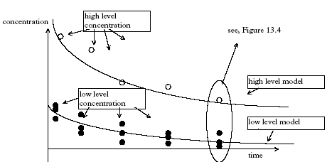
Figure 13.1 Princippet for det laminare lag mellem sediment og vandsøjle. Model 8, Degradation and transport in the sediment The degradation is assumed to take place in the sediment pore water, so Eq. 13.8 is used directly and combined with the initial and boundary conditions as described in Eqs. 13.18, 13.19a-c and 13.20, (model 3). 13.3 The relative complexity of the modelsThe relative complexity measure is used in order to find the most simple model if more than one model can describe the experimental data equally well. The most simple model is defined to be the least complex. The complexity level is defined as the number of model parameters necessary to calibrate. Thus, the complexity increases as the number of parameters increases. Examples of parameters could be the effective degradation coefficient (keff) and the diffusion coefficient (D). The models have different complexity levels and they are ranked in relation to each other in Figure 13.2. Figure 13.2 Modellerne rangordnet i relation til niveauet for kompleksitet. En parameter er en specifik koefficient i en ligning, f.eks. den effektive nedbrydningskoefficienten keff. 13.4 Solution and calibration methodology13.4.1 Solution methodologyThe models number 1 and 2 are solved by simple integration forming exponential functions. The more complicated models involving partial differential equations (SML and sediment transport) are solved numerically by an implicit finite difference solution (Crank, 1975) for the sediment and by explicit finite difference solution for the SML (Crank, 1975). All the partial differential equations in this investigation are linear so analytical solutions are possible, but they are complicated due to complicated boundary conditions. 13.4.2 Calibration methodologyStandard least square is doubtful Often in the model analysis the needed calibration is performed using two concentration series of different magnitude and different number of replicates, see Figure 11.3. In this case a standard least square method will tend to yield wrong weightings of the single data points in relation to each other. Consider the principal plot on Figure 13.3, which is of the same type as Figure 11.3, having two time series, one of single values and an other one of triple replicates. The high level concentration series represent single values, while the low level concentration series consist of triple values formed by three nearly equal values of dosage. Therefore, the low level series has a higher statistical power compared to the high level series and the low level series should have more weight in the model calibration than the higher level series. Furthermore, the variation (uncertainty) related to each data point may vary during time and between the two time series.
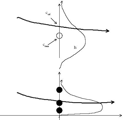
Figure 13.3 Principperne for den heterogene modelfitning, hvor tidsserien for de lave koncentrationsværdier er gentaget tre gange, mens tidsserien for de høje værdier er enkeltbestemmelser. It is critical to assure the right weighting for each data point in the model calibration algorithm in order to disclose the best model. The principle of improved calibration function The data points are interpreted as stochastic variables for every time step as illustrated in Figure 13.4. The uncertainty related to each data point is a result of both a "true" variability of the data and a lack of knowledge because of a limited number of measurements (here: one and three) at each time step and each concentration level. The data point weighting needs to split-up the uncertainty in these two different sources in order to include the difference between single values (less knowledge) and three replicates (more know-ledge).
Figure 13.4 Datapunkterne fortolket som stokastisk variable, der beskrevet ved tætheds-funktioner. Density functions The variability of a data point for a known parameter vector is denoted f and defined as follows (13.26)
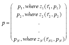
The f function consist of a parameter vector ( (13.27)
where The vector function The probability measure for c to be included in the distribution function at a specific value of General density function including parameter (13.28)
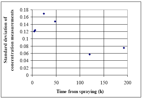
Where the argumentation is: The resulting probability for an event is equal the sum of all the probabilities yielding the event. In other words the probability for c to be included in the distribution function is the sum of all the probability values formed by all possible pi value combinations ending up in this integral equation. The form of Eq. 13.28 is general and the functional form of f and z has to be determined before Eq. 13.28 is useful. Selection of a normal distribution The function f is assumed to be normally distributed ( N(c,μ,σ) ). Thus, the parameter vector Estimation of standard deviation The estimation of s is done at different time steps using the low concentration series only, see Figure 13.5 for fenpropathrin. The first four values lies around 0.14, while the last two values decrease to about 0.07 and the decrease is expected from this type of decreasing concentration experiments. The standard deviation is a result of various uncertainty sources from the spraying, sampling and analysis activities so the standard variations at different time steps are partly correlated to each other. In this investigation the standard deviation is assumed to be a fixed value for the time below 50 h (0.14) and an other fixed value (0.07) for the time later than 50 h. Unfortunately, it is not possible to estimate the standard deviation for the high level concentration series because they only consist of single numbers. Information about the standard deviation for the low concentration series has to be used in order to estimate the standard deviation at high concentration levels. The standard deviation at high concentration level can be estimated from the low level series as: (1) equal to the low level standard deviation at same time step; (2) proportional to the concentration level by a factor calculated using the low level standard deviation. The choice of (1) or (2) must depend on the uncertainty source. If the uncertainty primarily arises from the analytic work in the laboratory, then the type (1) method is best, while if the uncertainty comes from the spraying and sampling activities and from heterogeneity between the two ponds the type (2) is preferable.
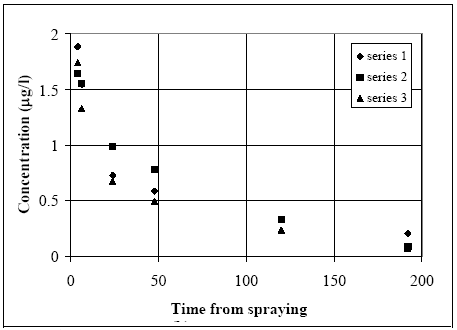
Figure 13.5 Standard afvigelserne til forskellige tider for tidsserien med fenpropathrin med de lave koncentrations værdier. If the heterogeneity between the ponds and dosage levels (spraying) were the dominating factor there should be a systematic difference between the three time series, see Figure 13.6. There seems to be some systematic difference between the time series indicating that the heterogeneity between the ponds and dosage levels are important for the standard deviation. The standard deviation for the high concentration level will therefore be estimated as proportional to the concentration level using the stand deviation at the low concentration level at the same time step.
Figure 13.6 Tidsserien for de lave koncentrationsværdier for fenpropathrin. The dosage level will be used as a measure for the concentration level yielding the following relationship between the standard deviation at the two concentration levels (13.29)
where σhigh and σlow are the standard deviations at high and low concen-tration levels, respectively, at the same time step. Combining Eq. 13.28 and the assumptions taken above yields the final density function as (13.30)
Final objective function The total accordance between a model calculation at the two concentration time series is given as (13.31)
where O is the finale objective function which needs to be optimized in order to find the best agreement between the model estimates and the measurements. M is the total number of comparisons between calculations and measurements, ccal,i is the calculated concentration at the i' the comparison. The h(ccal,i) value is the single comparison probability for a calculated concentration value to be included in one of the time series at a specific time step. The total probability for a model calculation to be "realistic" in relation to the total time series measurements must then be the product of all the single comparison probabilities yielding Eq. 16.31.
|
||||||||||||||||||||||||||||||||||||||||||||||||||||||||||||||||||||||||||


