|
Autonomous Weeder for Christmas Trees – Basic Development and Tests 5 Control system development
As already described in chapter 3 the basis for control of the ACW was a route plan and a tree location map, including positions of the field borders and a docking station. 5.1 RequirementsThe requirements to the control system were that the machine should:
5.1.1 Procedure of weeder operationAssuming that an ACW would have to weed several plantations a normal weeding operation would consist of tree steps:
When placed at the docking station and started up in autonomous mode it should first initialise, i.e. check if its location corresponds to the location of the plantation map allocated, or, alternatively, choose the plantation map and route plan appropriate for its present location. It should also check and initialise its own settings before starting up on the planned route through the plantation. After completion of the weeding it should return to the docking station and report back that the job has been done. It should also report back if any serious errors or faults have occurred during the operation. 5.1.2 Safety and reliabilityWhen operating commercially, the ACW should check for unexpected obstructions, major malfunctions, and classify its condition and reaction to one of the groups in table 5.1. If the coordinator wants to stop the ACW he should be able to do that just by activating an easily recognisable emergency button. 5.2 Control principlesAs already stated the ACW would need two main areas of control: The deterministic vehicle tracking control and the cutter positioning control. The route plan was used to control the movement of the vehicle, while the tree map was used to control the rotor cutter position relatively to the vehicle. Table 5.1. Safety modes, built in checks and reactions selected for the ACW control system.
5.2.1 Vehicle tracking controlThe principle of vehicle route plan tracking is shown in Fig. 5.1. The vehicle is controlled to follow the straight line between two waypoints until it crosses a set switch distance line. Then it starts to track the next line segment from P2 to P3, and so on, until the switch line of the last waypoint when it should stop.
Fig. 5.1. Line tracking principle. The vehicle tracks the line between two waypoints until the switch line. Then it tracks the next line. Another word for “switch distance” is “tolerance”. When the reference is updated (waypoints shifted) it will appear to the controller as a step function. The controller will do a “best effort” to track the reference. In case of a 90 degrees turn some deviation will occur due to the limits of the vehicle turning radius. The shape of the path can be adjusted by changing the “switch distance” or tolerance. The controller has a quite good smooth transfer between modes but there are limits. In other words, a 90 degrees turn with switch distance 0 when starting treatment in the middle of a row, should be avoided (since the path deviations will most likely cause the vehicle to drive into the trees). This is mainly done by starting the “inter-row strip center-line” tracking prior to the beginning of the row, or, in case treatment has to be started in the middle of the row, with a smooth approach (small change of vehicle heading). 5.2.2 Cutter positioning systemThe cutter mechanism (Fig. 4.5 and 4.6) could be controlled either passively or actively. In the passive mode (Fig. 5.2) it would be pulled out in its outer position by the spring. If the cutter in this position hits an obstruction, e.g. a tree trunk, it would be pressed back against the spring force and slide around the obstruction. In the active mode (Fig. 5.3) the control system would pull the cutter back when passing a tree, thus avoiding contact. 5.2.2.1 Passive cutter positioning If the vehicle always moves forward this approach could be used without an actuator for cutter arm positioning. All that is needed would be a route plan, which will take the ACW along the tree row at the proper distance with the cutter working in the intra row area sliding around the tree trunks. However, this system might cause problems of damage to newly planted trees which are less resistant to impact and wear. However, in older stands this might be an advantage because it might help to reduce the growth of the top shoot. The impact force exerted on the trees by the cutter would be proportional to the acceleration of the cutter, which would be proportional to the square of the forward speed. Therefore, speed is an important factor in the design of passive control.
Fig. 5.2 Time series showing cutter with passive control 5.2.2.2 Active cutter control In order to have contact free positioning of the cutter the actuator should pull it back from the intra-row area at the appropriate time when a tree is approaching, and restore its position relative to the row when the tree has been passed (Fig. 5.3).
Fig. 5.3. Time series showing cutter with active control 5.3 System architectureTo meet the above requirements to control the system the architecture shown in Fig. 5.4 and 5.5 was developed. It contains the three main functions:
The purpose of the VTC (Fig. 5.4) was to get the ACW to track the route plan so precisely that it would be possible to control the cutter sufficiently well. This was achieved on basis of a mathematical model of the vehicle dynamics, sensor inputs and optimization of the simulated response according to the principles described by (Omae, 1999). The simulated error was continuously minimized about 1 s ahead. This error was a function of the position, orientation, steering angle (all relative to the current reference line) and to the speed of the vehicle. In the current version the vehicle speed (throttle setting) is controlled by just two commands, i.e. a setting for start of the engine and a setting for working speed. When the throttle was set at working speed the engine speed was held fairly constant by a speed regulator. Thus the vehicle forward speed and the cutter speed were fairly constant. The VTC is further described in appendix A.
Fig. 5.4. Main elements and information flow of the vehicle tracking control (VTC), (top half) and weed cutter arm positioning control (WCP), (lower half) of the ACW system architecture. The objective of the WCP was to get the cutter to follow the desired route as shown in Fig. 5.3, i.e. it should be kept out in the proper position and not hit the trees when passing. The controller used was a simple quasi-static controller, i.e. when the calculated distance to a tree goes below a certain threshold the arm is pulled back from the row and vice versa. If the system for some reason fails to pull the cutter in, at the right time, the cutter will hit the tree trunk, and the passive cutter arm control will come into action. The objective of the VFR (Fig. 5.5) was to check for a number of faults and to generate an appropriate behavior as stated in Table 5.1. So far the system checks whether:
If any of these are false the control system would stop the engine. This function is facilitated by a closed-loop system that updates values at a frequency of 1 Hz for the navigation and 40 Hz for the cutter positioning. The controllers shown in Fig. 5.5 are only able to issue commands to the actuators when they are enabled. Thus the VFR will watch for error conditions and, in case of an error, disable the controllers and take over actuator commanding from the task specific controllers.
Fig. 5.5. Main elements and information flow of the vehicle fault and obstruction reaction system (VFR) in the ACW system architecture. 5.4 System hardware and information flowsAn overview of the system hardware is presented in Fig. 5.6. The control system was built around a 400 MHz embedded PC, which controls the actuators on basis of data from the sensors. Six actuators (LINAK) are operating the steering system, throttle, brake/clutch, gear, cutter arm position and cutter clutch. During operation the main parameter values were transferred through the WLAN-connection to a laptop computer using the “screen shot” function for the xPC Target. Also, the large number of parameter values sampled each cycle, were stored in a log for possible later uploading. These parameters could also be transferred in UDP (Ethernet) packets to any computer on the network for real-time access to the ACW status information. At this stage only Run/Stop command are used (from the laptop to the xPC Target).
Fig. 5.6. ACW hardware components and information flows. 5.4.1 Control panelA control panel was used for operation in joystick mode and sequencing prior to switching to Navigation mode. It consists of 3 buttons and 3 LED's as shown in Fig. 5.7.
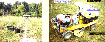
Fig. 5.7. Sketch of the ACW control panel. 5.4.2 Sensor systemsThe sensor systems used so far were a RTK GPS receiver, which was used to measure the absolute position, and a tilt-meter to measure vehicle tilt for corrections of vehicle position relative to the antenna position. The GPS antenna height was approx. 95 cm above the ground. Investigations on inclusion of more sensors, e.g. a laser range scanner for detection of tree rows and obstructions were also undertaken, but these sensors were not integrated with the ACW control system within this project. 5.4.2.1 Positioning The GPS used was a Trimble model MS750 (or rover for the ACW) and a MS7400 (for the base station). The rover was operated at 10 measurements per second in RTK-FIX-mode, i.e. the measured positions were corrected on basis of signals from the base station. The correction signals were transferred via radio modem (Satel model SATELLINE 3ASd, operating in the 380 to 470 MHz range). Fig. 5.8 shows how the components of the system were placed in the field and on the vehicle.
Fig. 5.8. Arrangement of reference station (left) and components on the ACW platform (right). 5.4.2.2 Laser range scanner Laser range scanners are able to measure distance and direction to objects. They can therefore be used to detect (and map) locations of objects in the surroundings (e.g. Guivant et al. 2000, Folkesson and Christensen, 2004). Holmgren (2003) applied a laser range scanner together with a simple GPS and an inertial navigation system to estimate forest variables. The system, which was carried by an aircraft, provided absolute positions of laser beam hits on trees and ground and a following sequence of data processes yielded good estimates of positions of individual trees, position of ground level, tree species, tree canopy volumes, tree height, stem position and thickness. In the present project an existing 2D laser range scanner (SICK LMS 200) was tested briefly to find out whether it would be suitable for detections of Christmas trees and obstructions. The purpose was to see if this scanner could be used to improve vehicle navigation and safety. 5.4.2.3 Tilt-meter The tilt-meter used (Applied Geomechanics, model MD900-TS) was mounted parallel to the ACW chassis (Fig. 5.8, right). The purpose of this sensor was to measure the vehicle pitch and roll, in order to calculate a correction to the vehicle position. 5.4.2.4 Position sensors in linear actuators All the actuators had built in potentiometers that sensed their length and thus via calibration functions could feed back information about the actual steering angle, gear ratio, clutch/brake position, engine speed (throttle setting), position of cutter and the state of the cutter clutch. A special supplementary electronic circuit was built to adapt these sensors to the control system requirements. The change in position when the actuator was energized was also used to determine whether the actuator had stalled. 5.4.2.5 Engine ignition sensor system The engine revolution was counted by a special circuit attached to the primary side of the ignition coil, and used by the control system to check the engine operation status. 5.4.3 Digital I/O adaptor and power circuitsThe embedded computer of the control system was connected to the sensors and actuators through a number of digital I/O adaptors comprising level conversion and frequency division. The ports on the I/O board (Diamond MM-32) were configured as 8 digital inputs (Fig. 5.9) and 16 digital output connections. The outputs were used for controlling the LINAKs (12), LED's (3) and a switch in the Safety Circuit chain (1).
Fig. 5.9. Digital inputs. 5.4.4 Power supply systemsAs the original electrical power system of the vehicle (17 Ah) was considered too noisy for the control system an additional 12 V battery (40 Ah) was mounted on the vehicle. This battery supplied power for the embedded computer and all the sensors, while the original battery supplied power for the actuators and basic vehicle functions. An overview of the power systems is shown in Fig. 5.10.
Fig. 5.10. ACW power circuits for engine ignition (bottom), actuators (middle) and high level electronics (top). 5.5 System softwareThis section presents the control software, including the principle of vehicle and tool control used, the vehicle fault and obstruction reaction system (VFR), the processing of sensor inputs, the tracking control, and the cutter positioning control. An overview of the information flows is shown in Fig. 5.4 and 5.5. 5.5.1 Processing of sensor dataThe GPS receiver and inclinometer outputs NMEA (National Marine Electronics Association) ASCII strings via an RS232 port. These strings are checked for errors and then, parsed by a specific C-function before being made available for the system. 5.5.1.1 GPS The Trimble GPS receiver outputs a string comprising time, date, northing, easting, GPS-quality, number of satellites, DOP (Dilution Of Precision), height and checksum on the serial port 10 times per second. If no errors were detected (Fig. 5.11) all messages were considered valid and passed on to the Simulink environment. In Simulink the GPS-quality value was evaluated. A value of 3 corresponds to RTKFIX-mode, the most precise mode and the only usable for centimetre level positioning. When the RTK-GPS is the only sensor for positioning, the vehicle should stop if the value differs from 3. This verification of the mode is done in a Stateflow chart, which makes it easy to shift to another GPS mode at a later stage. Also, a dynamic check was made of the measured positions to detect and remove outliers. This was done by applying a rule saying that the latest measured position had to be in close proximity to at least one of the previous two measurements to be accepted. The limit is configurable through a parameter in the specific block mask – and was set according to the vehicle maximum speed, maximum tilt rate and GPS antenna height. (If the tiltmeter were enabled, the filtered correction vectors were applied to the position, before it was distributed to the rest of the system). Apart from estimating the delays (when configuring the controller) and doing time-tag based filtering of the incoming instrument data, nothing was done with respect to synchronization of inputs. 5.5.1.2 Tilt-meter The inclinometer outputs a text string approx. 8 times per second. This string is converted and the values are range checked, written again and compared. The checksum is calculated and compared to the transmitted value. It appeared that heavy filtering of the tilt-meter output was needed to reduce the noise to an acceptable level. Thus the asynchronous arrival of tilt-meter messages (compared to GPS messages) was not a problem, as much as the delays in the noise filter. 5.5.1.3 Actuator position potentiometers The actuator potentiometers returned a voltage proportional to the length of the actuators. This voltage was transformed to the actual physical parameters like steering angle, gear number etc. by use of appropriate calibration constants. 5.5.2 Vehicle tracking controlThe principles of the vehicle tracking control are described in section 5.2.1. The details of this were that the tracking controller compared the current position (GPS-antenna) and heading of the ACW with the line between to waypoints (i.e. it calculates the cross track error and the heading relative to the line). The position of the vehicle was calculated on basis of the current position and recent history of positions, while the vehicle orientation was calculated and extrapolated also from recent history using dead reckoning based on speed and steering angle to compensate for the delay in the filter. Once an estimate for the current position and heading was obtained, the response (i.e. future position and heading) to a number of control pulses applied to the steering system were simulated, and the one expected to result in the least error was chosen. The pulses simulated were of different duration (i.e. time before the output returns to: (0) No change) and polarity: (1) Turn left, (-1) Turn right. All actuator settings were done by maximum speed of the actuator motor. Wheel slip was not considered. The Simulink block for all these processes is shown in Appendix A. 5.5.3 Cutter positioning controlTo get sufficiently accurate position estimates for the cutter position it is important to have an accurate estimate of the vehicle position, as well as a frequent update of the conditions, i.e. 40 Hz instead of the slower GPS update of 10 Hz. Also it would be important to have a minimum computer process time delay. The set up of this control is described further in Appendix B. 5.5.4 Safety systemThe purpose of the supervisory logics, which is described in Appendix C, is to have safe operation, i.e. make sure that the ACW will work only when conditions are safe and within normal ranges (table 5.1). For instance it should only be able to operate when in the right plantation, when it has a proper route plan, when the sensor inputs are received and they are of appropriate quality etc. 5.5.4.1 Geo Fence One of the safety blocks is "ValidField", which prevent the vehicle from driving if it is outside the field or plantation borders defined. The input to this block is the latest GPS position received. The output is a flag (boolean), stating whether the GPS position is within the field boundary or not. To ensure that this system works properly the route plan should always be defined within the limits of the geo fence. 5.5.4.2 Condition check block The "NavigationSuitable" block collects the relevant inputs and evaluates whether they would preclude Navigation mode (or Implement Task mode). The output is an error mask (Navigation Error Mask). If this mask is zero then everything is normal and Navigation mode is allowed. Otherwise a “bit” is set in the mask to signal, which condition failed. 5.5.4.3 Mode Sequencer The "ModeSequencer" block controls which of the low level controllers are enabled and what their objectives are (Table 5.2). Table 5.2. Overview of the actuator modes used
5.5.4.4 Actuator protection The actuators are only capable of intermittent use. If an actuator is blocked for some reason the current will increase and quickly cause overheating. To avoid this the actuators were protected by a two-level safety system: 1) A software controlled on/off switch (controlled on basis of detection of “actuator blocked” and a rough estimate of the motor temperature from “on-time”) that allowed continuous operation and avoided replacement of fuses, and 2) An ordinary thermal fuse in case the first level of protection should fail. 5.6 Simulink representationsThe Simulink diagram (Fig. 5.12) shows the top-level control loops in the ACW. Each of the boxes contains subsystems in several layers down to the hardware drivers. 5.7 Simulations and tests of the control systemDuring development, the function of the different elements and the whole control system were concurrently simulated in Simulink until they appeared to work properly. Then the vehicle part of the model was replaced by the real vehicle including the proper electronic connections, and tested physically. This was first done in a model of a Christmas tree plantation at the University Campus (Fig. 4.2, left) and then in a Christmas tree plantation with different sizes and types of trees. The model plantation at the campus was used for the initial trial and measurements of the spatial precision of the vehicles operation, while the real plantation was used for test of the practical performance of the weeder. The campus plantation model comprised 27 white plastic pipes placed in iron pipes that were fixed in the ground in the usual pattern for Christmas trees , i.e. 1.2 m between the rows and 1.2 m between the trees. Also 5 markers specifying the position of the docking station and the field boundary were set up according to the general definition (Fig. 3.4).
|