Market information in life cycle assessment5 Method for handling co-products5.1 Why system expansion is the preferred option for handling co-products5.2 Theoretical model for system expansion 5.3 A procedure for handling co-products 5.4 Identifying a product as determining for the volume of the co-producing process 5.5 Treating intermediate processes 5.6 Waste or co-product? 5.7 Recycling 5.8 Services as co-products 5.9 Complex situations 5.10 Traditional co-product allocation as a special case of the presented procedure 5.11 Relation to the procedure of ISO 14041 15 When a process or product system in an LCA is related to more than one product, it presents a problem: how should its exchanges, such as the resources consumed and the releases generated, be partitioned and distributed over the multiple products? The allocation of these multiple products, known as “co-products”, has been one of the most controversial issues in the development of the methodology for LCA, as it may significantly influence or even determine the result of the assessments. It has been seen as so central a procedure that it is often (even in the International Standards Organization standard on life cycle assessment, ISO14040) nick-named “allocation” as if it was the only allocation problem in LCA16. Allocation is the partitioning and distribution of an item over several other items. Co-product allocation is the partitioning and distribution of the exchanges (e.g., inputs and outputs) of a multi-product process over its co-products. The co-product allocation problem is parallel to the cost allocation problem, which has been extensively treated in the economic literature (a review pertinent to LCA is provided by Frischknecht 1998). However, while cost allocation is primarily an accounting tool where the different methods can be said to have each their advantages and disadvantages from the view of different decision makers focusing either on issues internal to their business or on direct business-to-business relations. In contrast, LCA begs for a solution that models as closely as possible all the external consequences of a potential change in demand for one of the co-products. The idea that co-product allocation can be avoided by system expansion has been put forward by Tillman et al. (1991) and Vigon et al. (1993) with respect to waste incineration, and more generally by Heintz & Baisnee (1992). System expansion is performed to maintain comparability of product systems in terms of product outputs, through balancing a change in output volume of a co-product that occurs only in one of the product systems, by adding an equivalent production in the other systems (or more elegantly and correctly by subtracting the equivalent production from the one system). For example, in the case of an LCA involving chlorine gas co-produced with sodium hydroxide used in another product system, the system is expanded with an alternative stand-alone production of sodium hydroxide, and the environmental releases and resource consumption of this alternative production is then subtracted from the system using the chlorine gas. System expansion was given a prominent place in the procedure of ISO 14041, where it reads in section 6.5.3: “Step 1: Wherever possible, allocation shall be avoided by: 1) dividing the unit process to be allocated into two or more sub-processes and collecting the input and output data related to these sub-processes; 2) expanding the product system to include the additional functions related to the co-products ”. Although avoiding allocation is seen as the preferable option, it has generally been regarded as impossible to expand the system in all cases. Therefore, other options have been maintained, especially the allocation according to the revenue or gross margin from the products, a procedure commonly applied in cost accounting (Huppes 1992). Older studies used simple physical allocation criteria such as the relative mass or exergy of the products, but these criteria have generally been discredited for lack of justification (Huppes & Schneider 1994), except in attributional, non-comparative LCAs, where they may still be used as a proxy for revenue. The following four obstacles to system expansion can be seen as part of the reason why this option has not generally been applied as a way to avoid allocation:
In this chapter, it is shown that allocation can (and shall) always be avoided in consequential LCAs. In attributional LCAs, it is not possible to express an imperative regarding what allocation procedure to apply, but avoiding allocation may still be an option. We reach this conclusion by demonstrating how to overcome the four obstacles listed above:
In the following sections it is demonstrated how system expansion is performed, with a number of examples. Special emphasis is placed on issues that have earlier been in focus of the allocation debate: joint production of e.g. chlorine and sodium hydroxide, zinc and heavy metals; the handling of “near-to-waste” by-products; and credits for material recycling and downcycling. It is shown that all the different co-product situations can be covered by the same theoretical model and the same procedure. Separate sections deal with the issues of uncertainty, co-product allocation as a special case of system expansion, and comparison to the procedure of ISO 14041. 5.1 Why system expansion is the preferred option for handling co-productsTo study correctly the effects of a potential product substitution in consequential, comparative LCAs, it is necessary that the studied product systems:
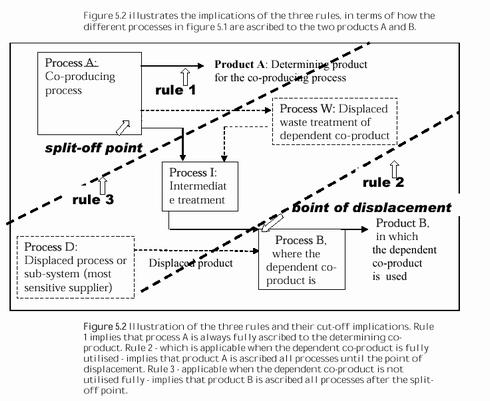
In general, these two conditions are not fulfilled by allocation. First, allocation typically involves a more or less arbitrary partitioning of the co-producing process over its co-products, without consideration of the extent to which a change in the amount of these co-products actually affects the functional output and other exchanges of the co-producing process. Secondly, allocation ignores the effects that a co-product may have on the further fate of the other co-products, i.e. displacement effects and additional treatment of the co-products before displacement takes place. Thus, traditional co-product allocation only fulfils the above two conditions in those particular instances where the allocation factors are chosen to reflect the way the co-products actually affect the co-producing process and where there are no significant effects on the further fate of the other co-products. In such instances, allocation may be regarded as a special instance of system expansion, as described in section 5.10. The above two conditions are fulfilled by system expansion, because any process, which will be affected by a change in the amount of co-products, is included in the studied product systems, and it is ensured that all systems yield comparable product outputs, by subtracting or balancing processes that do not occur in all of the compared systems (for details, see the procedure described in later sections). This is the rationale for preferring system expansion to allocation for handling co-products in prospective LCAs. In a non-comparative, attributional LCA, the preference for system expansion (as in the ISO procedure) still leads to a reasonable result, when the study is understood as an analysis of hypothetical historical changes like: What would have happened if this product had not been introduced or if this product had been produced instead of this? In this case, historical market data can be used to calculate hypothetical system expansions and to show what the results would have been of a prospective LCA if it had been produced at that historical moment. 5.2 Theoretical model for system expansionSystem expansion is illustrated in figure 5.1 showing a co-producing process with one determining co-product (product A); that is, a co-product that determines the production volume of that process. This is not necessarily the co-product of interest to the specific life cycle study. In figure 5.1, just one dependent co-product is shown, but in practice there may be any number of co-products. That a product is determining for the production volume of a process is the same as saying that this process will be affected by a change in demand for this product, as identified by the procedure in chapter 4. Performing a system expansion in relation to joint production is to answer the question: How will the production volume and exchanges of the processes in figure 5.1 be affected by a change in demand for the co-product that is used in the life cycle study? Because the environmental exchanges are generally linked to the production volumes, the answer to this question will also provide a solution to the allocation issue. This question is equally relevant when the co-product used in the life cycle study is the determining product for the co-producing process (A) and when it is the product in which the dependent co-product is utilised (B). A complete identification of changes in production volume as a function of change in demand would require an economic model for all the involved processes and product flows. The procedure presented here involves the simplifying assumption that a change in demand for a dependent co-product does not affect the production volume of the co-producing process17. Under this assumption, the answer to the above question can be summarised in three rules18:
It may at first sight appear counter-intuitive that the intermediate process is ascribed to product A when product B utilises all of a dependent co-product, while the process is ascribed to product B when only part of the co-product is used in product B. This is a reflection and a good illustration of the difference between the (more intuitive?) attributional perspective that focus on the average behaviour (full utilisation or not) of the intermediate process rather than on the consequences of this full utilisation for the changes in the volume of the intermediate process when demand for product B changes, which is the focus of the consequential approach upon which the three rules are based. 5.3 A procedure for handling co-productsFigure 5.3 presents a procedure for handling co-products in the form of a flow-chart. An initial distinction can be made between joint production, where the relative output volume of the co-products is fixed, and combined production with independently variable output volumes (Huppes 1992). For the latter type of production, allocation can be avoided simply by modeling directly the consequences of a change in the output of the co-product of interest (that which is used in the product system under study) without change in the output of the other co-products. This situation is dealt with in step 1 of the procedure. The remaining part of the procedure (steps 2 to 4) deals with the situation of joint production where allocation can only be avoided through system expansion. For combined production, a physical parameter can generally be identified, which - in a given situation – is the limiting parameter for the co-production. It is the contribution of the co-product of interest to this parameter, which determines the consequences of the studied change. In the guideline (Weidema 2003), two examples are provided of this: treated surface area of product plus border area in a combined surface treatment, and weight or volume in different situations of combined transport. Here we add an example of a combined freezer/refrigerator and the classical example of combined treatment of several wastes in the same treatment plant (e.g. landfill or incinerator):
Example: Example: The limiting production parameter may depend on the original situation. Therefore, it is essential to describe both the original situation in terms of the relative outputs of the co-products before the studied change, and the production parameters that in this situation are determining the changes in the exchanges of the combined production. This is even more obvious when the output of the co-products can only be varied within certain limits, that is, when the production cannot be separated completely. In many production processes where one raw material is used to produce several outputs, the production parameters can be adjusted to give different relative yields of the co-products, but only within certain limits. When operating close to such a limit, the consequences of the studied change may be ambiguous, and this should be reflected in the modeling and its results.
Example:
Example: As already suggested by the last example, some productions may appear as allowing individual variation in output, but when subjected to a closer analysis it is only possible to keep the output of the other co-products constant by adjusting sub-processes not involved in the original production. Thus, what appears at the superficial level to be a case of individually variable co-products may in fact be a joint production requiring a system expansion (steps 2-4 of the procedure, see below). Example: 5.4 Identifying a product as determining for the volume of the co-producing processWhen the output of the co-products cannot be independently varied, a change in demand for one of the co-products may or may not lead to an increase in the production volume of the co-producing process. This depends on whether the co-product in question is determining for the production volume or not. Identifying a product from a joint production (to keep it short, such a co-product will simply be called a joint product in the remaining part of this section) as determining for the production volume of the co-producing process is the same as showing that the co-producing process will be affected by a change in demand for this specific co-product (which we will then call a determining co-product for short). When the co-producing process is identified as the affected process by using the procedure in chapter 4, we have in fact at the same time identified the co-product under study as being a determining co-product. For a co-product, the crucial point in the procedure in chapter 4 is the identification of the other co-products as a production constraint. The production volume of the co-producing process is constrained by the demand for the determining joint product(s). Independently variable (combined) co-products cannot provide a constraint and may be simultaneously determining (as described in the previous step). In this section, it is explained:
The overall production volume of a co-producing process is typically determined by the combined revenue from all the co-products, since production of an additional unit will be profitable as long as the total marginal revenue exceeds or equals the marginal production costs. As a starting point, this also implies that any change in revenue for any co-product may affect the production volume. Thus, to identify a joint product as determining, it is adequate to document that a change in demand for the joint product leads to a change in revenue for the co-producing process. However, as already discussed in section 2.4, the default assumption in life cycle assessment is that suppliers are price-takers and the long-term market price of a co-product is therefore typically determined by the long-term marginal production costs of the alternative production route for this co-product, if such an alternative route exists. As long as the price of a joint product and thus its contribution to the overall revenue of the co-producing process is determined by its alternative production route, a change in demand for this co-product will not lead to a change in its (long-term) price and there will be no change in its contribution to the overall (long-term) revenue of the co-producing process. Thus, there is typically only one of the joint products that is determining at any given moment. This understanding can be further elaborated into the following two conditions: To be a determining co-product, a joint product (or a combination of joint products in which the co-product takes part) shall:
Note that the stated market trends and revenues are relative to the normalised output volumes of the co-producing process, which means that differences in the actual physical quantities have already been eliminated. At a marginal production cost for the co-producing process of 9, only one co-product (A) can provide adequate revenue to change the production volume alone. Product C cannot alone influence the production volume, in spite of the large market trend for this product. However, the combination B and C also fulfil the condition of providing adequate revenue. The possible influence on the production volume from this combination is determined by the smallest of the market trends of the products in the combination. This is the medium trend of product B. Because this is still larger than the trend of product A, product B becomes the co-product that determines the production volume. Condition ii) above implies that if more than one joint product or combination of joint products fulfil condition i), then only that joint product or combination which has the relatively largest change in overall demand (market trend) is actually determining. This again emphasises that as long as alternative production routes exist for the joint products, there is only one of the joint products that can be determining for the production volume at any given moment.
Example: Example: For joint products that do not have any relevant alternative production routes, their prices will adjust so that all the joint products have the same normalised market trend, since only then the market will be cleared. In this situation, a change in demand for one of the joint products will influence the production volume of the joint production in proportion to its share in the gross margin of the joint production. This is equivalent to the result of an economic allocation. However, the resulting change in output of the other joint products influences their further downstream lifecycles, including their consumption and disposal phases, and thus requires the inclusion of the processes affected. This latter aspect of system expansion is ignored in a pure economic allocation of the joint production (see also section 5.10).
Example: The above theoretical illustration with the 4 joint products A,B,C, and D, also shows that the determining co-product is not necessarily the co-product that yields the largest revenue to the process (although this will often be the case), and that the determining co-product is not necessarily the co-product that is having the largest increase (or decrease) in demand. It should be obvious that the two conditions above, and thus the determining co-product, may change over time, depending on location and the scale of change. Thus, it is always important to note the preconditions under which a given co-product has been identified as determining. When in doubt, or when conditions vary within the studied scale or geographical or temporal horizon, two or more alternative scenarios should be modelled. 5.5 Treating intermediate processesThe intermediate processes are those processes that take place between the split-off point where a dependent co-product leaves the processing route of the determining co-product and the point of displacement where the dependent co-product can displace another product (see also figure 5.2). While it is always relevant to determine the split-off point, it is only relevant to determine a point of displacement when the dependent co-product is utilised fully in other processes and actually displaces other products there. The determining co-product for the intermediate processes is identified by investigating whether the condition of rule no. 2 (section 5.2) is fulfilled or not, i.e. whether the dependent co-product is utilised fully in other processes. If the condition is fulfilled, the volume of intermediate treatment (and the amount of product being displaced) depends on the product volume of dependent co-product. Since the co-products cannot be independently varied, this volume is fixed by the determining product of the co-producing process. A change in demand for the dependent co-product will not lead to any change in the intermediate treatment (exactly because it is not determining, i.e. it cannot affect the volume of the co-producing process). Thus, the intermediate treatment and the co-producing process have the same determining product, and (as stated by rule no. 2) the intermediate process shall be fully ascribed to this product.
Example: Since in this situation, where the dependent co-product is fully utilised, it is the determining product for the co-producing process that also determines the amount of product being displaced, this product shall also be ascribed other possible changes resulting from the displacement. This applies to the changes in the alternative raw material supply, as in the example above, where the determining product for the co-producing process is ascribed (credited for) the changes in the displaced process, but also to such changes in the further life cycle of the dependent co-product that are a consequence of differences between the dependent co-products and the products they displace.
Example: Compared to the displaced raw material, the dependent co-product may contain a contamination, e.g. of heavy metals, which gives it a different performance during the final waste treatment of the product in which the dependent co-product is used. The difference in waste treatment and/or in environmental exchanges form the waste treatment shall be ascribed to the determining product for the co-producing process. If, in the described situation where the dependent co-product is fully utilised, no point of displacement can be found, i.e. if the dependent co-product cannot immediately displace another product, the entire life cycle of the product in which the dependent co-product is used can be regarded as belonging to the intermediate treatment. Alternatively, it can be regarded as an alternative (but not necessarily more environmentally benign) waste treatment for the co-producing process. Both of these perspectives implies that the volume of the product in which the dependent co-product is used depends on the supply from the co-producing process, and that all processes in the life cycles for both the determining and the dependent co-products are to be ascribed to the determining product for the co-producing process. As the dependent co-product has a function (else it would be a waste) the resulting product system is strictly speaking still a system with more than one function. In spite of this, it is comparable to other product systems that solely yield the determining product. These other product systems shall not be expanded with the additional function (the one yielded by the dependent co-product) since this function is solely caused by the existence of the dependent product and not by any external demand19.
Example:
If the condition of full utilisation is not fulfilled, it means that part of the dependent co-product is treated as a waste. In this situation, the volume of the intermediate treatment (and the displacement of waste treatment) is determined by how much is utilised in the receiving system, and not by how much is produced in the co-producing process. Thus, the product in which the dependent co-product is used, is determining the volume of the intermediate processes and shall be ascribed these (while being credited for the avoided waste treatment), as stated by rule no. 3 (section 5.2).
Example:
Example: As illustrated by the examples, whether a co-product is utilised fully and whether it displaces other products, depend on market conditions that may change:
Thus, it is important always to note the conditions under which the determinant for the intermediate processes has been identified. If the investigated change is of such a size that it in itself changes the conditions for the system expansion, i.e. changes which product is determining or whether the dependent co-product is utilised fully, the system expansion shall be calculated on the basis of the resulting conditions after the change. The information needed to determine whether a dependent co-product is fully utilised are obtained from market and waste statistics and market studies, often available in-house in the involved industries. If it is uncertain whether this condition is fulfilled, it may be necessary to apply different scenarios to reflect the limited knowledge. 5.6 Waste or co-product?In previously presented allocation procedures, it was important to distinguish between wastes and co-products, because the exchanges of the co-producing process should be allocated over the co-products, but not over the wastes and emissions. Waste is often defined in vague terms as ’outputs that need further treatment’ (see e.g., Frischknecht 1994) or ’outputs that the holder discards or intends to or is required to discard’ (EEC 1991) supported by exemplary or authoritative listings (e.g., the European Waste Catalogue 1994). In a more stringent way, waste can be defined as economic inputs and outputs (as opposed to inputs and outputs from and to the environment) with a value equal to or lower than zero (see e.g., Huppes 1994). In the procedure presented here, the distinction between wastes and co-products is not important. If in doubt whether an output is a waste or a co-product, the output can be regarded as a dependent co-product and passed through the procedure. It will then fall under either rule 2 (the treatment of wastes that do not displace any other products would then be classified as an intermediate treatment and ascribed to the determining product for the co-producing process, just as a waste treatment would normally) or rule 3 (for “near-to-wastes” that are not fully utilised) of section 5.2. If a waste in the economic sense, i.e. an output without economic value to the process that produces it, displaces another product, the “waste treatment” is in fact a recycling, and rules 2 or 3 should therefore be applied in order to model correctly the consequences of this “waste treatment”. Thus, from the procedure presented here, a novel definition of waste may therefore be derived: A waste is a dependent output that does not displace any other product. This definition is in line with the intention of the definition in the European Waste Directive (EEC 1991) but gives a more precise distinction. 5.7 RecyclingRecycling has been regarded as presenting distinct allocation problems needing a separate treatment (for a number of articles on this topic, see Huppes & Schneider 1994). Examples of specific allocation procedures developed to handle recycling situations are the 50/50 rule (Ekvall 1994) and the material grade model (Wenzel 1998, Werner & Richter 2000). However, the procedure presented earlier in this chapter is applicable for recycling, as for any other situation in which the same processes are shared by several products. In the recycling situation, it is not difficult to identify the determining process for the primary life cycle. This is obviously the product of this life cycle, not the scrap. The central issue is what determines the recycling rate and thus the degree to which the scrap is utilised in the secondary life cycle. In an expanding market for the scrap product, such as is the case for most metals, all scrap collected will be used. In this situation, a change in the volume of the primary life cycle will lead to a change in the amount of scrap available for collection, and a change in the amount collected, and a change in the amount of scrap utilised in secondary life cycles, and thus in the displacement of “virgin” production (i.e. following rule 2 of section 5.2). A change in the volume of the secondary life cycle will not be able to influence the amount of scrap utilised, because it is already utilised fully. Thus, the change in the volume of the secondary life cycle must be covered by a change in “virgin” production (i.e. still following rule 2). However, it should be noted that a change in demand for scrap products may have indirect effects in the form of political intervention, reinforcing the signal sent by the change in demand, as also described in section 4.3. Such indirect effects are possible when significant quantities of scrap are available for collection, in addition to the amount already collected, and the costs of the additional collection is comparable to the costs of extracting “virgin” material. Such indirect effects should be described in separate scenarios, since they depend on political decisions that are difficult to predict. In immature markets, the recycling might be below the economic optimum due to capacity constraints. In this situation, neither using nor supplying scrap will affect the recycling rate. An increase in demand will thus affect “virgin” supply, while an increase in supply to recycling will increase waste deposits. Only a specific action to remove the capacity constraints on recycling will effectively increase recycling. Also in this situation, a specific demand for scrap products may have long-term indirect effects that may be modelled in separate scenarios, as noted in the previous paragraph.In a shrinking market, as we see for cadmium and some other heavy metals, some of the available material is being deposited, because there is not an adequate demand. A change in volume of the primary life cycle will only lead to a change in the amount of material to be deposited, whereas a change in the volume of the secondary life cycle will lead to a change in the amount being recycled, and thus indirectly also to a change in the amount being deposited (i.e. following rule 3 of section 5.2). It is interesting to note that in the case of cadmium (and possibly other heavy metals) the amount of recycling is fixed by environmental regulation, which means that it is “virgin” cadmium (as a by-product from zinc production) that is deposited, whereas in other situations it can be expected that it is the scrap material that would not be collected. It may be argued that the studied changes in either the primary or secondary life cycle may also have a secondary effect on the market prices, and that this would equally affect the price of the primary product and of the collected scrap. This was the background for the so-called 50/50-rule suggested by Ekvall (1994) under the assumption that the supply elasticities of the “virgin” production and scrap were equal (i.e. that they would react to a price change with the same change in volume). Actually, the price elasticities are not equal (Ekvall 1999), and at the high recycling rates that exist in free markets with low entry costs (where the value of scrap is determined by the marginal cost of “virgin” production), the resulting volume change in collection is likely to be much less (probably often negligible) compared to the change in “virgin” production. This would support the above conclusion of applying rule 2 in the situation of expanding markets. Also in the case of a moderately shrinking market, where the supply from “virgin” production still plays a role, the difference in supply elasticities would imply that the “virgin” production will be affected most. However, in a rapidly shrinking market, the scrap can cover the entire demand and virgin supply would not be relevant. In this situation, a small change in volume of the secondary life cycle would only be able to affect the scrap collection, which is in line with our above conclusion of applying rule 3 in case of shrinking markets. One of the reasons that recycling has been thought to demand a separate allocation procedure has been that - when the recycling rate is below its environmental optimum - both the user of scrap materials and the supplier of scrap may need an incentive to increase recycling, and that it is therefore important that the environmental advantage of increased use of recycled materials is distributed over the actors in the way that actually stimulates an increase the recycling rate. Furthermore, as the same material may be used over and over again in several consecutive life cycles, it has been seen as “unfair” if only the first or the last life cycle should carry the burdens of extraction and waste treatment. The procedure presented here provides a clear cut-off between the individual life cycles, determined by whether there is an inflow of “virgin” material or not. In an expanding market, all life cycles affect the amount of “virgin” material extraction, and only the production that ensures an increase in the collection (by providing more material for recycling, or by specifically increasing recycling capacity, either technically, by economic support in parallel to the option of cross-subsidising suggested in section 4.3, or by stimulating political intervention) will be credited for the resulting increase in recycling (displacement of “virgin” extraction and decrease in waste handling). In a decreasing market without “virgin” inflow, all life cycles that utilise scrap products will be credited for the resulting increase in recycling (decrease in waste handling), and no life cycle will be credited for supplying additional material to recycling (since this would just mean that an equivalent amount would require waste treatment elsewhere). In this way, the procedure does not provide support for general incentives for using or supplying scrap, but provides an incentive for using scrap when the market for the material in question is decreasing, and for supplying scrap when the market is expanding, which is exactly what is needed to increase recycling in these two respective situations. When the recycling rate is below its environmental optimum, the procedure furthermore gives credit for specific actions that increase recycling capacity. In some situations, the recycled material cannot displace “virgin” material, either because its technical properties have been reduced (e.g., paper fibres that become shorter for each recycling, so that after approximately six cycles they are so short that they must be discarded), or because it has been contaminated (e.g. copper in iron scrap, and silicon alloys of aluminium that cannot be recycled with the ordinary aluminium scrap). In these cases, sometimes described as downcycling, several distinct markets may exist for different qualities of recycled material, and the displacements that will occur will be determined by the supply and demand on these markets. If a demand for a specific scrap quality is not satisfied completely, scrap of higher quality or virgin material may be used, while scrap of lower quality cannot be used. When upstream processes deliver more scrap than the capacity of its downstream markets, some of the scrap will not be used. Thus:
A change in demand for a specific product, produced with scrap material, will cause both of the above. In the case of contamination of virgin material, it should be noted that it is not only the current market situation that must be considered, but rather a very long-term market situation. As long as the current demand for scrap qualities is larger than the supply, all the contaminated scrap will be used and will displace “virgin” material. The contamination will be diluted due to the constant inflow of virgin material. However, at some stage in the future the scrap markets may become saturated, so that the contamination becomes a limitation for the recycling (this is already happening with copper contamination in iron scrap). The current contamination may thus lead to a future need for waste treatment of the contaminated material, or at least to a different displacement than on the current market (see e.g. Kakudate et al. 2000, Holmberg et al. 2001). It is this future market situation that should be used to determine what processes to include in the system expansion, since the immediate displacement of “virgin” material is only a temporary postponement of the necessary supply of “virgin” material in the future situation, when the contaminated material can no longer be used. The need to take into account these future effects is included in the third sentence of rule no. 2 of Box 3: “If there are differences between a dependent co-product and the product it displaces, and if these differences cause any changes in the further life cycles in which the co-product is used, these changes shall likewise be ascribed to product A.” For materials where the technical properties are reduced on recycling, each additional life cycle will imply a change in the quality of the material in the recycling pools, influencing the requirements for supplies of “virgin” material to the pools. The need for new material may be caused e.g. by degradation of fibres or polymers, as can be seen with paper or plastics. Thereby, the change in material quality may also be expressed as a change in the ability of the material to displace “virgin” material. A life cycle that delivers as much material to recycling as it receives will cause a change in material quality equivalent to the amount of “virgin” material supply that is needed to compensate for the reduction in technical properties. When less material is sent to recycling than what is received (i.e. when material is sent to waste treatment), the change in requirements for supplies of “virgin” material to the recycling pool (the change in displacement ability) will depend on the actual quality of the material that is thereby leaving the recycling systems. The quality (the ability to displace “virgin” material) can be estimated specifically by the physical properties or be calculated theoretically from the average recycling rate in the specific recycling pool, since the material quality will be reverse proportional to the recycling rate (with a low recycling rate the supplies of “virgin” material will be relatively large, which gives a relatively high material quality in the recycling pool – and opposite with a high recycling rate). The EDIP’97-method (Wenzel et al. 1997) applies a factor, called the grade loss, to express the loss of grade or material quality on recycling. This grade loss is used as an allocation factor, in that every life cycle using the material is burdened with this fraction of the primary material production. The grade loss is calculated as the percentage of virgin material that must be introduced on recycling. Therefore, in terms of system expansion, the grade loss is equivalent to the difference between the amount used in a lifecycle and the amount displaced by the recycling from this life cycle, expressed in percentage of the amount used, i.e. the change in displacement ability as explained in the previous paragraph. Thus, given the same information on displacement, the EDIP‘97-procedure will lead to the same result as the procedure presented here. Note, however, that he EDIP’97-method does not take into account the situation where the recycling pools are not utilised fully, which implies e.g. that in EDIP’97 the recycling process is always ascribed to the preceding life cycle.
Example: 5.8 Services as co-productsThe situation where the co-products are services (e.g., waste treatment or transport) has also been regarded as presenting distinct allocation problems, also known as multi-input allocation because the co-products are typically related to physical inputs to the process (e.g., the waste to be treated, or the goods to be transported). In the procedure presented here, the same method is used for service products as for material products (goods). The typical examples used are combined transport and combined waste treatment. It appears that most service outputs supplied to multiple product systems can be independently varied, and therefore treated already by step 1 of the procedure (see figure 5.3). However, we have been able to find at least one example of a joint waste treatment service that requires the use of system expansion (joint neutralisation of waste acids and bases):
Example: Secondary functions of forestry and agriculture, such as maintaining rural income and maintenance of landscapes for recreation, may also be used as examples of service co-products that can be treated by the procedure in complete parallel to physical products. As the name implies, these functions are typically secondary compared to the production of physical products. Thus, the secondary functions may be regarded as non-determining co-products, while the physical product (e.g. wheat or wood) is typically the determining product. The demand for the physical product can change either as a result of changes in the market or changes in crop specific subsidies. In both cases, the fulfilment of the secondary functions is affected (e.g. causing changes in rural income or landscape maintenance compared to the desired output of these functions). This change may or may not be counteracted by alternative measures, but can in both situations be covered by rule no. 2 of section 5.2. The affected alternative measure (i.e. the most sensitive measure for supporting rural income or for landscape maintenance, respectively) depends on the current policies in the specific situation. In some situations, the so-called secondary functions may in fact be the primary concern, e.g. when rural income support is administered per land area or when landscape maintenance is rewarded without requirements to what crops should be grown. If this source of income leads to changes in the production, the subsequent change in composition of product output may be one of the side-effects that has to be accounted for by including the alternative production displaced. This may involve a number of subsequent changes on different markets. 5.9 Complex situationsThe situation described by figure 5.1 is a simplification, in that it shows only one determining and one dependent co-product (i.e. only two products coming out of process A) and none of the other processes have co-products. Therefore, this section deals with the more complex situations:
More than two co-products seems to be rather the rule than the exception when processes have more than one product, as can be seen from most of the examples in the previous sections. This, however, poses no problem for the procedure. Each co-product can be treated separately:
Multiple products resulting from an intermediate process (i.e. a process occurring after the split-off point and before displacing other products) means that the dependent co-product is split up in two or more fractions, each following its own route. Each fraction may be fully utilised in other processes (rule no. 2 of section 5.2) or only partly (rule no. 3). Each fraction can be treated separately, although fractions that follow the same rule may be treated together for convenience (listing the affected products and processes together). Even when the co-product is not composed of separable fractions, it may have many different applications. Then, the process to be considered in the system expansion is the application most sensitive to a change in supply (as identified by the procedure in chapter 4).
Displaced processes that have multiple products, of which the displaced product is only one, will require a repetition of the procedure for each of the co-products from the displaced process. If this leads again to another process with multiple products, as illustrated in figure 5.4, one might fear that this system expansion would continue without end. However, the number of possible processes involved in the system expansion is limited by the very procedure, since:
Example: In Weidema (2003) an example is provided of an iterative solution of the joint production of ethylene and propylene from steam-cracking, where an additional output of ethylene yields also an output of propylene, the displaced production of which again leads to a by-product of ethylene and so on. Below, a similar example with joint production of protein and vegetable oil is given. This example was first published in Weidema (1999).
Example: This may also be expressed as the solution to a system of linear equations. If the products are named a and b, the suffixes A and B signify the originating processes, and the 1 represents the desired product output: This is simply a specific case of the general solution for a life cycle inventory with the normalised output of 1 unit of a. While the system described above is limited to the product outputs from the co-producing and displaced processes, a standard product system include also the upstream and downstream processes and their product flows (product inputs to a downstream processes expressed as negative amounts in the downstream process). Therefore, the solution can be generalised to any number of products a, b, c, etc. and any number of processes A, B C. etc. Below an example is provided with 5 interdependent fishery processes which all produce two or more of the 5 fish products. This shows that any complexity of co-products can be handled simply by including the affected processes in the product system and using the standard procedure for solving the system (by either iteration or matrix reduction). The most difficult part is thus not the mathematical solution, but the identification of the affected processes and the acquisition of environmental data for these processes. As part of the Dutch methodology project (Guinée et al. 2001), we had the opportunity to show how the procedure presented in this chapter compares to an economic allocation of the same relatively complex system, namely that of a (hypothetical, simplified) refinery, both receiving co-products (waste from other processes) and supplying a number of both joint and combined co-products. This example (first published in Guinée et al. 2001, part 2b, pp. 36-41 where our method was named “symmetrical substitution method”) is reproduced in annex A, while the economic allocation of the same refinery process can be found in Guinée (2001, part 2b, pp. 32-35). 5.10 Traditional co-product allocation as a special case of the presented procedureIn traditional co-product allocation, the exchanges of the co-producing process is partitioned and distributed over all the co-products according to a product specific allocation factor between 0 and 1, and there is no inclusion of intermediate and displaced processes. Expressed in the terms of consequential LCA, this implies that for any co-product, the co-producing process is assumed to react to an increase in demand with an increase in production volume in proportion to the product specific allocation factor. For example, a demand of 1000 kg of a co-product with the allocation factor 0.1 will lead to an increase in production volume of the co-producing process resulting in an increase in output of 100 kg of the demanded co-product. This further implies that the remaining part of the demand (here 900 kg) is covered by an alternative supply and/or a reduction in consumption elsewhere, and that the environmental impacts of this are assumed negligible, since the system is not expanded to include this alternative supply and/or changed consumption and related processes. In a joint production, the increased production volume of the co-producing process implies an equivalent increase in the output of the other joint products. In traditional co-product allocation, since the system is not expanded to include the further fate of these joint products (displacement of alternative supply, increase in consumption and/or waste handling), the implied assumption is that this further fate is having negligible environmental impacts. This may lead to serious inconsistencies when the alternative supply, consumption or waste handling is included elsewhere in the same product system. For example, in a product recipe using both sunflower oil and soy beans, a traditional allocation of the sunflower production would allocate part of the sunflower production to the sunflower protein cake, but not include the soy production displaced by this additional supply of sunflower protein, while the same soy production would be included for the soy beans used directly in the recipe. However, there may be situations in which the reaction of the co-producing process to an increase in demand for its co-products is proportional to specific allocation factors, and where at the same time neither alternative supply, consumption, nor waste handling of the co-products will be affected. This is the case when:
Thus, in such a situation, the traditional co-product allocation may be regarded as a special case of the procedure in figure 3.2. As mentioned in section 5.4, several joint products may influence the production volume of a joint production in proportion to their share in the gross margin of the joint production, when the normalised market trend of all the joint products is aligned as a result of constraints in alternative production routes. In this situation, co-product allocation according to gross margin may correctly reflect the way the co-producing process will be affected. However, as there is no storage of co-products (exactly because the markets are cleared), intermediate treatment and consumption of the co-products will be affected, and the co-product allocation must be supplemented by a system expansion with the affected processes. As a more academic question, it may be asked whether the entire procedure presented in this chapter could be called “co-product allocation,” rather than a way to avoid allocation. This basically depends on the original viewpoint. If the co-products and their further fate are originally regarded as being outside the studied system, it is reasonable to regard the presented procedure (in which the changes in the processes affected by the change in amount of co-products are added or subtracted from the studied system) as a way to avoid allocation. If the originally studied system is regarded as including the co-products (and their further fate, as well as the processes that the co-products may displace), the presented procedure can be regarded as an allocation of the different changes in production volumes over the different co-products. The word “ascribed” in the four rules can be replaced by “allocated”, and the procedure of “crediting” can be understood as “allocating the decrease in production volume to”. In that case, the term “system expansion” is a misnomer, and should preferably be named “market-based allocation”. In the ISO standard 14041, system expansion is regarded as a way to avoid allocation, and we have therefore maintained this viewpoint in the present chapter. Step 1 in the procedure in figure 5.3 (dealing with combined production) is equivalent to step 2 in the ISO procedure (allocation according to physical relationships), but because the output of all other co-products are kept constant, these co-products may as well be regarded as being originally outside the studied system, meaning that there is no allocation problem. The entire presented procedure can therefore be regarded as “avoiding allocation.” 5.11 Relation to the procedure of ISO 14041Because – as shown in this chapter – system expansion is always possible for cases of joint production in consequential LCA studies, the stepwise procedure of ISO 14041 (ISO 14041, clause 6.5.3) will lead to the same results as the procedure presented in figure 5.3:
Since each step in the ISO procedure can be related to a specific group of cases (step 1: joint production in consequential studies; step 2: combined production in consequential studies; step 3: attributional studies) the step-wise nature of the ISO procedure is unnecessary. Simply describing the application area of each step in the procedure, as suggested here, would give a more straightforward presentation. In the procedure presented in this article, step 1 deals with combined production (ISO step 2), while steps 2 to 4 deals with system expansion (ISO step 1), because it appears more logical to deal first with the simple case, where the outputs of the other co-products can be kept constant without system expansion, before dealing with the more complicated cases, where the outputs of the other co-products can only be kept constant by applying system expansion. However, in practice the order does not matter. If applying system expansion to a case of combined production, the same result will be obtained as when applying the simpler procedure of step 1 of the procedure presented in this article. In fact, step 1 can be treated as a special case of the model for system expansion if the limiting parameter for the combined production is seen as the determining co-product, and the non-limiting parameters as the dependent co-products.
Example: Step 2 of the ISO procedure may also be regarded as a special case of the very first procedural step of the ISO procedure, which we have ignored in the above presentation, namely the obvious option of avoiding allocation by subdividing the process into sub-processes that only produce one product. Such a subdivision is obviously not possible for joint production as is mainly relevant when “black box” data have been collected for a production that is in fact an aggregate of independent production lines. However, in consequential LCA, combined production may be regarded as such independent production lines, since it is possible to measure the independent reaction of the co-producing process to variation in output of each co-product separately. When step 2 of the ISO procedure is regarded as describing special cases of either process subdivision or system expansion (both termed “avoiding allocation” in ISO 14041), it would be more relevant to include it in step 1, before the description of system expansion, i.e. resulting in the same order as in the procedure in figure 5.3. Besides the three-step procedure, ISO 14041 (section 6.5.2) prescribes an allocation principle, which has popularly become known as “the 100% rule”: “The sum of the allocated inputs and outputs of a unit process shall equal the unallocated inputs and outputs of the unit process”, i.e. there should not be any exchanges that are allocated twice or not allocated at all. Although, according to the ISO text, this principle applies only to allocation and not to avoiding allocation, it is worth noting that the procedure presented in this article adheres to this principle: The three rules in section 5.2 ensure that all processes are fully ascribed to (allocated to) either one or the other co-product. ____________________________________________________________
|