| Bottom | | Front page |

Environmental project no. 1003, 2005

The indoor and outdoor concentrations of particulate air-pollution and PAHs in different size fractions and assessment of exposure and health impacts in the Copenhagen population

Contents

Preface

Summary and conclusions

Sammenfatning og Konklusion

• Baggrund og formål
• Undersøgelsen
• Hovedkonklusioner
• Projektresultater

1 Introduction

• 1.1 Background
• 1.2 Purpose of the study

2 Experimental methods

• 2.1 Sampling conditions
• 2.2 Description of field sites
• 2.2.1 The Jagtvej apartment (Jagtvej_IN)
• 2.2.2 The Jagtvej street canyon (Jagtvej_EXT)
• 2.2.3 The National Institute of Occupational Health, Denmark (NIOH)
• 2.3 Indoor and outdoor meteorology
• 2.4 Collection of particulate matter and volatile compounds
• 2.4.1 Collection of PM1, PM2.5 and Inhalable dust
• 2.4.2 Collection of volatile compounds
• 2.5 Analysis of PAHs
• 2.5.1 Pressurized Liquid Extraction of glass fibre filters and Tenax TA
• 2.5.2 High Performance Liquid Chromatography (HPLC) analysis

3 PM in indoor and outdoor air

• 3.1 PM1, PM2.5 and PMinh
• 3.1.1 Intrasite relationships and prediction of missing PM data
• 3.1.2 Outdoor-outdoor relationships and prediction of missing data
• 3.1.3 The contribution from traffic to the particulate air-pollution
• 3.1.4 Indoor-outdoor relationships
• 3.2 Seasonal variation and comparison with PM guidelines
• 3.2.1 Seasonal variation
• 3.2.2 Comparison with air-pollution guidelines
• 3.3 Evaluation of particle induced health effects
• 3.3.1 Assessment of adverse health effects related to PM2.5
• 3.3.2 Increase per million per 10 g/m3 increase in PM2.5
• 3.3.3 Health effect assessment based on the PM2.5 distribution function

4 PAHs in indoor and outdoor air

• 4.1 Evaluation and description of PAH-concentrations
• 4.1.1 Distribution of PAHs on the glass fibre filters and Tenax TA
• 4.1.2 Artifacts influencing the measured concentrations of PAHs
• 4.1.3 Occurrence of the measured PAHs
• 4.2 Indoor-outdoor relationships for PAHs associated with PM2.5
• 4.2.1 Street to background relationships
• 4.2.2 Indoor-outdoor relationships
• 4.2.3 The contribution from traffic to PAHs in the indoor air
• 4.3 Seasonal variation of the PAH concentrations
• 4.4 Health effect evaluation based on the PAH measurements

5 Conclusions

6 Reference list

Appendix A

• Meteorological wind data

Appendix B

• Description of collection methods and filter weighing procedure
• PM measurements
• Filter cleaning and weighing procedure
• Mass-Loss Correction for Mass Concentration Measurements

Appendix C

• List of PAH names, abbreviations, structures, etc.

Appendix D

• Analysis of PAHs
• Solvents and standards
• Sample preparation
• Pressurized Liquid Extraction (PLE) of filters and Tenax TA
• High Performance Liquid Chromatography (HPLC) analysis of extracts
• Gas chromatography combined with mass spectrometry (GC-MS)
• Validation of the method
• Data treatment

Appendix E

• HPLC raw data tables - PAH concentrations in extracts from filters. Tenax TA sample and backup tubes and blanks

Appendix F

• Tables of measured concentrations of PAHs in indoor, outdoor and urban background air

Preface

The overall goal of this study was to update our present knowledge of the indoor and outdoor air-pollution in central Copenhagen (Denmark), to investigate the importance of the infiltration of traffic generated air pollution to the indoor environment in a case-study apartment, as well as to assess the potential adverse health effects in the Copenhagen population. The measures in the study was fine (PM₁ and PM_2.5) and coarse (inhalable dust) particulate air-pollution and sixteen volatile and semivolatile polycyclic aromatic hydrocarbons associated with the particles.

The project was financed by the Danish Environmental Protection Agency (Danish EPA) and established as an extension of Work-Package C3.1 under the Centre for Traffic Research on environmental and health Impacts and Policy, TRIP (http://www.akf.dk/trip/index.htm).

The project was followed by an observation group consisting of:

- Poul Bo Larsen, Danish Environmental Protection Agency (chairman)

- Christian Lange Fog, Danish Environmental Protection Agency

- Ole Hertel, National Environmental Research Institute

- Marianne Glasius, National Environmental Research Institute

- Steffen Loft, University of Copenhagen

FieL_Dwork was conducted between January and July of 2002 in close collaboration with the TRIP WP3.1C Working Group from the National Environmental Research Institute (Roskilde), The Danish Building and Urban Research Institute (Helsingør), The Danish Environmental Protection Agency, University of Copenhagen and The National Institute of Occupational Health (Copenhagen).

The current project was conducted and reported by a working group at the National Institute of Occupational Health, Denmark, which consisted of Vivi Kofoed-Sørensen, Per Axel Clausen and Keld Alstrup Jensen. Dorte Narv and Tina Trankjær Olsen additionally supported with technical assistance during the fieL_D campaigns.

During the course of this study we have had fruitful discussions with the observation group who also reviewed the current report. Additionally, we are grateful for beneficial discussions on the HPLC method with Åse-Marie Hansen and Dorrit Meincke.

Summary and conclusions

Fifteen one-week samples of PM₁, PM_2.5, inhalable dust (PM_inh) and 16 polycyclic aromatic hydrocarbons (PAHs) were collected inside and outside of an uninhabited 4^th floor apartment at the Jagtvej street canyon in central Copenhagen during winter, spring and summer in 2002. Similar urban background samples were collected at a 2 km distant 4^th floor high rooftop. PAHs in PM₁ and PM_inh were collected on glass fibre filters only. PAHs in PM_2.5 were collected on glass fibre filters followed by adsorbent sample and backup tubes containing Tenax. PM was determined by filter weighing. The PAHs were analyzed by liquid extraction of filters and adsorbent tubes followed by high performance liquid chromatography with UV and fluorescence detection.

The Copenhagen particulate air-pollution was dominated by fine particles. App. 70 wt% of the PM_2.5 consisted of PM₁ at all sites. The average PM_2.5 content in PM_inh was 54 and 69 wt% at Jagtvej and in the urban background, respectively. Indoors PM_inh consisted almost entirely of PM_2.5. Correlation analysis showed a strong relationship between PM₁, PM_2.5 and PM_inh at Jagtvej and in the urban background. However, PM at Jagtvej exceeded the urban background concentrations. The difference suggests that traffic on average contributed with 3.5±1.9 g/m³, 5.0±2.7 g/m³ and 14.6±4.0 g/m³ to PM₁, PM_2.5 and PM_inh, respectively.

Indoor PM correlated well with PM in both the street and the urban background. However, indoor-outdoor ratios below unity (0.77±0.21 for PM₁ and 0.77±0.24 for PM_2.5) were only achieved using PM-concentrations measured in the street at Jagtvej. The average indoor PM_2.5 concentration (15.20 μg/m³) exceeded the annual indoor PM_2.5 concentration of 15 μg/m³, which is recommended in the US based on the US-EPA air-quality guideline for PM_2.5. At the best, the outdoor PM_2.5 concentrations (19.80 μg/m³ at Jagtvej and 14.85 μg/m³ in the urban background) just complied with the target values proposed by the EU CAFE Working Group to be within 12 to 20 μg/m³. Assessment of adverse health effects induced by PM_2.5 at 95% CI suggested 780520 excess accumulated deaths per million in Copenhagen in 2002. Additionally, 1556701 excess hospitalisations were predicted per million inhabitants for respiratory symptoms and all cardiovascular disease, combined.

In PM_2.5 samples the total concentrations of the 16 US-EPA gas and particle phase priority PAHs (ΣPAH) were 15-284 ng/m³ indoors, 46-235 ng/m³ outdoors, and 2-105 ng/m³ in the urban background. The concentrations were probably underestimated due to extraction recovery below 100%, breakthrough, and reaction with ozone and nitrogen oxides during sampling. The real concentrations may be up to two times higher than observed. Urban background, traffic and indoor sources contributed to the overall concentration of PAHs in the uninhabited apartment. Traffic in the Jagtvej street canyon and indoor sources appeared to be the most important sources for PAHs indoors. The WHO unit risk value of 8.7 10^-5 per ng/m³ B(a)P for life-time cancer risk suggests that ~10 cancer cases per 106 inhabitants may occur at a life-time exposure to the PAH-concentrations observed in the apartment. For comparison, 8 and 5 cases per 10⁶ inhabitants are expected from the street and urban background concentrations, respectively. B(a)P may be an inadequate marker for assessment of cancer induced by urban air-pollution. Differences between indoor and outdoor PAH profiles and presence of other carcinogenic compounds may result in serious estimation errors.

Sammenfatning og Konklusion

• Baggrund og formål
• Undersøgelsen
• Hovedkonklusioner
• Projektresultater

Sundhedsskadelige partikler og tjærestoffer fra biltrafikken trænger ind i selv husenes øverste etager langs trafikerede gader i København. Forureningen med fine partikler er mindre end grænseværdien foreslået af EU, men kan alligevel betyde ca. 780 for tidlige dødsfald om året i Storkøbenhavn. Koncentrationen af de målte kræftfremkaldende tjærestoffer er lav og ser ud til kun at have ringe betydning for udvikling af lungekræft. Dette er nogle af resultaterne fra en undersøgelse af partikler og tjærestoffer i luften indenfor og udenfor en ubeboet 3. sals lejlighed på Jagtvej i København. I undersøgelsen blev der fokuseret på indtrængning af udendørsforureningen ind i lejligheden og vurdering af helbredseffekter.

Baggrund og formål

Videnskabelige undersøgelser har vist, at jo højere luftforureningen med små partikler er i byerne, desto flere dødsfald og hospitalsindlæggelser er der pga. især hjertekarsygdomme, luftvejsproblemer og kræft. Imidlertid ved man, at det ikke partiklerne alene der er årsag til de flere dødsfald. Nogle af indholdsstofferne er skadelige i sig selv. Blandt de mest omtalte indholdsstoffer er de kræftfremkaldende tjærestoffer. Disse stoffer dannes ved forbrænding af organisk materiale. Forbrænding af fossile brændstoffer som kul, olie, diesel og benzin er formodentlig den vigtigste kilde til tjærestoffer i luften i Danmark. Indendørs er rygning og madlavning vigtige kilder til luftforureningen med tjærestoffer.

Partiklernes evne til at trænge ind i bygninger og deres biologiske effekter varierer med partiklernes størrelse. Små partikler med en diameter på under én mikrometer kan let trænge ind i en bygning og kan inhaleres langt ned i menneskers lunger. Tjærestofferne findes hovedsageligt i disse små partikler. Imidlertid kan partikler med tiden enten optage eller afgive gasser til omgivelserne og klumpe sammen, hvorved deres masse og størrelse ændres. Derfor er det uklart hvor meget af udendørs partikelforureningen der faktisk trænger ind i bygninger. Formålet med projektet var at måle koncentrationen af partikler og tjærestoffer i luften udenfor og indenfor i en lejlighed, for at kunne vurdere den faktiske indtrængning af disse trafikforureninger i bygninger.

Undersøgelsen

Undersøgelsen, der blev foretaget af Arbejdsmiljøinstituttet, blev baseret på luftprøver opsamlet indenfor og udenfor en ubeboet tredje-sals-lejlighed på en trafikeret gade (Jagtvej) i København i løbet vinter, forår og sommer 2002. Der blev opsamlet i alt 15 én-uges luftprøver af tre forskellige partikelstørrelser i de tre kampagner af hver fem ugers varighed. Prøverne skulle bruges til bestemmelse af luftforureningen med partikler og 16 forskellige tjærestoffer (Polycyclic Aromatic Hydrocarbons: PAHer). Tilsvarende prøver af bybaggrundsluften blev indsamlet i tredje sals højde på Arbejdsmiljøinstituttets tag, ca. 2 km fra lejligheden. Meget fine partikler (PM₁; partikler mindre end 1 mikrometer), fine (PM_2.5; partikler mindre end 2,5 mikrometer) og inhalerbare partikler (PM_inh; partikler op til ca. 100 mikrometer) blev opsamlet på filtre. Gasformige PAHer blev desuden opsamlet på et specielt gasfilter monteret efter partikelfiltret til indsamling af PM_2.5. Koncentrationen af de opsamlede partikler blev målt ved vejning af filtrene. PAH'erne blev målt ved at udtrække dem fra partikel- og gas-filtre med et opløsningsmiddel og efterfølgende analysere udtrækket med specialinstrumenter.

Hovedkonklusioner

Biltrafikken forurener luften med partikler og tjærestoffer på Jagtvej i København. Denne forurening trænger ind i den undersøgte tredje-sals-lejlighed på Jagtvej. I lejligheden var der også andre kilder til luftforurening med partikler og tjærestoffer. Denne forurening kunne være indtrængning af udendørsforurening igennem nabolejligheder eller forurening fra nabo-lejlighederne, hvor der f.eks. blev lavet mad eller røget. Den gennemsnitlige koncentration af fine partikler (PM_2.5) på Jagtvej (19.80 mikrogram per m³) og i bybaggrunden (14.85 mikrogram per m³) lå i grænseområdet sammenlignet med de årlige middelkoncentrationer på 12 til 20 mikrogram per kubikmeter, som diskuteres i den såkaldte CAFE arbejdsgruppe i EU. Baseret på PM_2.5 ser den fine partikelforurening ud til at kunne betyde ca. 780 (95CI: 260 – 1300) for tidlige dødsfald om året i Storkøbenhavn. Alle målinger af tjærestoffet benzo(a)pyren var under den nyligt vedtagne EU-målværdi på 1 nanogram benzo(a)pyren per kubikmeter. De målte koncentrationer af tjærestoffer ser da heller ikke ud til at kunne betyde mere end ti kræftdødsfald i hele Storkøbenhavn over en 70-årig periode. Benzo(a)pyren er måske ikke tilstrækkelig til at vurdere kræftrisikoen ved den atmosfæriske luftforurening. Det kan skyldes at sammensætningen af tjærestoffer i de forskellige miljøer varierer for meget. Desuden kan partikler indeholde andre kræftfremkaldende stoffer og evt. i sig selv forstærke den kræftfremkaldende effekt. Det tager den velaccepterede benzo(a)pyren model ikke højde for.

Projektresultater

Den københavnske luftforurening viste sig at være domineret af fine partikler. Cirka 70% af PM_2.5 bestod af PM₁. Det gennemsnitlige indhold af PM_2.5 i PM_inh var henholdsvis 54% og 69% udendørs på Jagtvej og i bybaggrunden. PM_inh i den ubeboede lejlighed bestod næsten udelukkende af PM_2.5. Der var en stærk sammenhæng mellem PM₁, PM_2.5 og PM_inh på Jagtvej og i bybaggrunden. Partikelkoncentrationen på Jagtvej var dog højere end i bybaggrunden og forskellen tyder på at trafikken i gennemsnit bidrog med 3.5±1.9, 5.0±2.7 og 14.6±4.0 mikrogram per kubikmeter til henholdsvis PM₁, PM_2.5 and PM_inh.

Forholdet mellem partikler indendørs og udendørs

Indendørs partikelforureningen varierede klart med udendørs-koncentrationerne både på Jagtvej og i bybaggrundsluften. Imidlertid var de gennemsnitlige indendørs/udendørs-forhold for PM₁ (0.77±0.21) og PM_2.5 (0.77±0.24) kun mindre end én, når indendørskoncentrationerne blev sammenlignet med partikel-koncentrationerne på Jagtvej. Inde-ude forholdet var derimod tæt på én for både PM₁ (1.120.34) og PM_2.5 (1.050.35), når man sammenlignede med ders koncentrationen i bybaggrundsluften. Da mennesker mest opholder sig indendørs kan den sammenhæng måske forklare, hvorfor data for forureningen i bybaggrunden kan anvendes i epidemiologiske studier af helbredseffekter forårsaget af luftforurening.

Indendørs og udendørs grænseværdier for partikler

I relation til grænseværdier og vejledninger for partikulære luftforureninger, så overskred den gennemsnitlige indendørskoncentration af PM_2.5 (15.2±5.0 mikrogram per kubikmeter) amerikanske anbefalinger for en årlig middelværdi for PM_2.5 på 15.0 mikrogram per kubikmeter i indeklimaet. Det skal her bemærkes, at vi må antage at gennemsnittet af de 15 én-ugers målinger kan ekstrapoleres til årsgennemsnit. Den gennemsnitlige udendørskoncentration i bybaggrunden (14.9±6.0 mikrogram per kubikmeter) og på Jagtvej (19.8±7.7 mikrogram per kubikmeter) var under den maksimale årlig gennemsnits målværdi på 20 mikrogram per kubikmeter, som er foreslået af CAFE arbejdsgruppen i EU. Koncentrationerne oversteg dog alle steder klart CAFE-gruppens laveste foreslåede årlige gennemsnits målværdi på 12 mikrogram per kubikmeter.

Vurdering af de fine partiklers helbredseffekter

Selvom luftforeningen i gennemsnit ligger på den rigtige side af den foreslåede grænseværdi, så viser en vurdering af helbredseffekterne som funktion af PM_2.5, at luftforureningen stadig medfører adskillelige tidlige dødsfald og indlæggelser. Beregninger vha. dosis-respons forhold fra Verdenssundhedsorganisationen (WHO) og førende amerikanske forskere viser, at der for hver million indbyggere årligt kan være 780 (95CI: 250 – 1300) for tidlige dødsfald i alt og ca. 1560 (95CI: 860 – 2260) ekstra indlæggelser på grund af hjertekarsygdomme og luftvejsproblemer baseret på koncentrationerne i bybaggrunden. De fleste af indlæggelserne (1006; 95CI: 305-1707) er forventet at skyldes hjertekarsygdomme.

Koncentrationen af PAHer i luften

Den totale koncentration af de 16 undersøgte PAH'er (ΣPAH) i PM_2.5-prøverne var 15-284 nanogram per kubikmeter indendørs, 46-235 nanogram per kubikmeter udendørs på Jagtvej, og 2-105 nanogram per kubikmeter i bybaggrunden. Koncentrationerne skal sandsynligvis betragtes som minimumsværdier, da man sjældent kan udtrække PAHerne 100% fra prøverne. Desuden kan der ske nedbrydning af PAHerne ved reaktion med nitrogenoxider og ozon under prøvetagningen. De virkelige koncentrationer kan være op til 2 gange højere.

Hvor kommer PAHerne i indeklimaet fra?

Både bybaggrunden, trafik på Jagtvej og indendørs kilder bidrog til PAH forureningen i den ubeboede lejlighed. De to sidstnævnte kilder var de vigtigste. Specielt var der en klar lineær sammenhæng mellem indendørskoncentrationen af tre partikelbundne PAHer (chrysene+benzo(b)fluoranthene+benzo(k)flouranthene), som er sporstoffer fra diesel, og udendørskoncentrationen på Jagtvej. Denne sammenhæng var der ikke, når deres koncentration i bybaggrundsluften blev brugt og viser at trafikken på Jagtvej spiller en væsentlig rolle for PAH og partikelforureningen inde i den undersøgte lejlighed. Indendørskilderne viste størst udslag for de gasformige PAHer, som evt. stammer fra rygning og madlavning i andre lejligheder i bygningen.

Kræftrisikoen fra PAH

Kræftrisikoen fra PAHer bliver normalt vurderet udfra koncentrationen af benzo(a)pyren. WHO's værdi på 8.7 10^-5 per nanogram per kubikmeter benzo(a)pyren for risiko for udvikling af kræft antyder, at der kan opstå ~10 kræfttilfælde for hver million indbyggere ved livstidseksponering for PAH-koncentrationerne målt i lejligheden. Tilsvarende kan ca. 8 og 5 kræfttilfælde forventes for hver million indbyggere fra gade og bybaggrunds-koncentrationerne. Benzo(a)pyren er måske uegnet til at vurdere den samlede kræftrisiko ved udsættelse for den atmosfæriske luftforurening. Det kan skyldes udsættelse for andre kræftfremkaldende stoffer og medhjælpende irritation fra partikler i lungen.

1 Introduction

• 1.1 Background
• 1.2 Purpose of the study

1.1 Background

Epidemiological studies have shown a relationship between increased mass concentrations of urban air-pollution and increased hospitalisation for respiratory symptoms and mortality rates (e.g.,Künzli et al. 2000; Schwartz et al. 2001; Schwartz et al. 2002; Pope, III et al. 2002; Nafstad et al. 2004)). These adverse health effects are better correlated to fine particles (PM₁ and PM_2.5) ^[1] than coarser particle measures (e.g., PM₁₀).

However, adverse health effects from air-pollution are not related to particle mass-concentrations alone. Long-term exposure to specific Hazardeous Air-Pollution Substances - often referred to as HAPS or air toxics - can also result in negative health effects of which cancer appears to be the most important outcome. In the USA, 188 HAPS' have been identified under the Clean Air Act Amendments of 1990 (http://www.epa.gov/ttn/atw/188polls.html). Among these air toxics, benzene and PAH's (Polycyclic Aromatic Hydrocarbon) are some of the most important carcinogenic compounds.

Combustion of fossil fuels (coal, oil, diesel and gasoline) is generally the most important source of PAHs in ambient air. Increased use of wood-burning stoves for domestic heating in Denmark has additionally re-introduced wood burning as an important PAH source in local environments . PAHs also exist as constituents in emissions from typical indoor sources such as cooking, smoking and indoor emissions from wood-burning stoves. Hence, human exposure to particulate matter and PAHs in indoor environments is a mixture of the contribution from outdoor air and that emitted from indoor sources.

The transport properties and biological effects from exposure to particulate air-pollution strongly depend on particle size distribution. Submicrometer particles can easily penetrate into the indoor environment, especially if air-filtration does not occur.

PAH's mainly occur in the fine particle fraction (Schnelle et al., 1995). A recent study has shown that the size distribution of PAH's at the 20 m roof-top in Saitama (Japan) was unimodal with a peak concentration at 480-680 nm . On the other hand, the maximum in relative PAH-contents was found in the particulate matter smaller than 200 nm. This is consistent with observations in exhaust from combustion of fossil fuels, where it has been found that PAHs form individual particles or adsorb onto especially the ultra-fine combustion particles during cooling of the flue gas or exhaust. Hence, owing to the size of combustion particles and production of volatile PAHs from e.g. traffic and other outdoor sources, PAHs may be an important constituent of the particulate air pollution indoors. Several studies have already been completed to quantify the degree of particle infiltration. However, owing to particle phase transformations and potential influence of indoor sources, it is still unclear to what extent urban air-pollution de facto penetrates into the indoor environment. Indoor-outdoor ratios of specific urban air-pollution compounds, such as PAHs, may yieL_D better estimates.

In addition to the infiltration efficiency into Buildings, particle size also determines the deposition efficiency of particles in the respiratory system. In humans, coarse particles deposit in the upper respiratory system, whereas the fine (PM₁ and PM_2.5) and ultrafine particles ( ≤ 100 nm) predominantly are retained in the deeper bronchioalveolar region of the lung. Some ultrafine particles also deposit in the nose and throat owing to their high diffusion rates. Consequently, since indoor particulate air-pollution and vehicle exhaust including particle-bound PAHs mainly occur in the submicrometer range, they are predicted to deposit mainly in the gas-exchange region in the deeper respiratory tract with lesser amounts in the nose and throat. Therefore, bias may occur in causal studies using coarser mass-dose estimates

1.2 Purpose of the study

The purpose of this study was to:

1. Determine the concentrations and indoor-outdoor relationship for PM₁, PM_2.5 and inhalable dust indoors and outdoors of an uninhabited apartment at Jagtvej in the centre of Great Copenhagen combined with roof-top measurements of urban background concentrations at the National Institute of Occupational Health (Copenhagen, Denmark).
2. Determine the concentrations and indoor-outdoor relationships for specific volatile and semivolatile PAH's in PM_2.5 at the three sample sites with focus on the influence from traffic air-pollution on indoor air.
3. Evaluate the potential adverse health effects induced by the particulate air-pollution and the carcinogenic risk induced by the observed PAH-concentrations in the indoor and outdoor environments in Copenhagen.

The project was funded by the Danish Environmental Protection Agency and conducted in synergy with the TRIP-project (Centre for Traffic Research on environmental and health Impacts and Policy) funded by the Strategic Environmental Research Program (http://www.akf.dk/trip/index.htm) and a parallel study of the characterization, inflammatory potential and genotoxic effect of the particulate air-pollution in Copenhagen funded by the Danish Ministry of the Interior and Health, Research Centre for Environmental Health (J.nr. 383-29-2001).

Footnotes

[1] PM is short for Particulate Matter. PM₁ is the mass concentration of particles up to 1 m-size.

2 Experimental methods

• 2.1 Sampling conditions
• 2.2 Description of field sites
• 2.2.1 The Jagtvej apartment (Jagtvej_IN)
• 2.2.2 The Jagtvej street canyon (Jagtvej_EXT)
• 2.2.3 The National Institute of Occupational Health, Denmark (NIOH)
• 2.3 Indoor and outdoor meteorology
• 2.4 Collection of particulate matter and volatile compounds
• 2.4.1 Collection of PM1, PM2.5 and Inhalable dust
• 2.4.2 Collection of volatile compounds
• 2.5 Analysis of PAHs
• 2.5.1 Pressurized Liquid Extraction of glass fibre filters and Tenax TA
• 2.5.2 High Performance Liquid Chromatography (HPLC) analysis

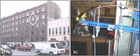
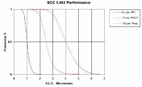
2.1 Sampling conditions

One-week samples of PM₁, PM_2.5, PM_inh (inhalable dust) and PAH's were collected from three locations at two fieL_D sites (Fig. 2.1): Indoors and immediately outside the living room window of a 4^th floor uninhabited apartment at Jagtvej, 2200 Nørrebro, Copenhagen, Denmark and at the 4^th floor-high roof-top of the National Institute of Occupational Health (NIOH), Lersø Parkallé, DK-2100 Copenhagen, Denmark.

Click here to see the Figure

Figure 2.1: Map showing the location of the fieL_D sites in the study and placement of city train tracks and crematories, which are potential local particle and/or PAH near the fieL_D sites.

All samples were collected during three fieL_D campaigns in 2002 covering winter (Jan 9 – Febr 13), spring (March 27 – May 8) and early summer (May 29 – June 26). The first two fieL_D campaigns were conducted contemporaneously with the last two multi-instrumental fieL_D campaigns in the national research project called TRIP (http://www.akf.dk/trip/index.htm). It was not possible to obtain samples during fall as the sublet contract of the apartment ended June 2002.

2.2 Description of fieL_D sites

2.2.1 The Jagtvej apartment (Jagtvej_IN)

Indoor particulate and PAH air-pollution were sampled in a furnished uninhabited 35.3 net m2 apartment. The apartment was located at the fourth floor (3. sal, tv.) in a residential Building at Jagtvej 83, in the central part of Copenhagen, Denmark (Fig. 2.1).

Figure 2.1: a) Picture of the apartment façade at Jagtvej. The encircled living-room window indicates the apartment used for the study. b) Image of the PM samplers mounted 1.5 m above the floor in the living-room, ~1.5 m from the living-room window. The CIS sampler is seen in the middle between the two Triplex cyclones for collection of PM₁ and PM_2.5. Tenax tubes are mounted in line after the PM_2.5 sampler on the right hand side.

The Building was erected around 1900 and has five stories with dwellings. The basement contains shops and storage rooms. The outer walls were masonry and ~32 cm thick story-partitions were made of wood with a layer of clay in between floor planks and underlying basal floor planks. In 1984 the Building was renovated with mechanical exhaust-only ventilation connected to kitchens and bathrooms. The centralized heating system connected to municipality district heating is from the same period. Heating was maintained using radiators with thermostats placed under the windows. New double glazed windows had been installed in well-sealed new frames around 1995.

During the fieL_D campaigns, the apartment and mechanical ventilation was modified by inserting a false door, sealing of the kitchen area, where all pumps and computer equipment were stored (Fig. 2.2). Tubes and wires were led through drilled and sealed holes in the false door structure. Taping door-cracks, keyholes and the mail slit in the entrance hall with gaffa tape minimized ventilation through the entrance door to the hallway.

Owing to the construction type with wooden floors and the recent replacement of pipes for the central heating system, story-partitions could not be expected to be airtight. The new windows, on the hand other were very airtight. Therefore ventilation slits were inserted in the street-ward window to allow higher fresh-air ventilation rates to levels closer to of at least 0.5 h¹ satisfying the Danish Building regulations. Despite this modification, results from the TRIP-project suggest that a significant amount of replacement air may enter the studied apartment through neighboring dwellings. Less than 20% of the replacement air entered directly from the street through the designated ventilation slits). Therefore, there is a high risk of contamination of especially volatile compounds from neighbour activities.

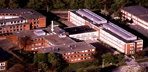
Figure 2.2: Sketch of the Jagtvej apartment with location of the indoor and outdoor sampling locations. The kitchen was sealed of by inserting an air-tight false door between the hallway and the kitchen. Air-exchange through the front door was sought eliminated by taping of the mail-slit, key-hole and the edges around the door.

2.2.2 The Jagtvej street canyon (Jagtvej_EXT)

Outdoor particulate and PAH air-pollution were sampled in the Jagtvej street canyon at 4^th floor height immediately outside the living room window of the uninhabited apartment (Fig. 2.2). Jagtvej is a NW-SE oriented two-way street with a traffic load on the order of 26,000 vehicles per working day of which approximately 6 % of the traffic is heavy traffic. In the monitoring area, the street canyon is partially open owing to the presence of a small street perpendicular to Jagtvej and a lower Building opposite of the apartment complex.

The samplers were mounted outside the living room window, placed next to each other appr. 10-15 cm apart shielded from direct sunlight at rain by a white hard-plastic bucket. Great care was taken to ensure that the sample inlet was well free of the shelter.

There was no apparent risk of sample contamination from proximate outdoor particles or PAH point sources at the 4^th floor sampling height. However, at ground level, a bus stop was located on both sides of the street in front of the monitored Building complex. Additionally, the near-by intersection between Jagtvej and Nørreallé (Fig. 2.1), which is another densely trafficked city road in Copenhagen, also may play a role on the local air-pollution levels. At 4^th floor height, however, these local effects are thought to be highly diluted and be of negligible importance as compared to the general traffic-load on Jagtvej senso stricto.

2.2.3 The National Institute of Occupational Health, Denmark (NIOH)

Urban background particulate and PAH air-pollution were sampled at the 4^th floor roof-top height of the National Institute of Occupational Health (NIOH) lecture hall (Fig. 2.3). The NIOH is located at the NW-SE oriented Lersø Parkallé 105, DK-2100 Copenhagen (Fig. 2.1).

Figure 2.3: Photo of the National Institute of Occupational Health, Denmark showing where the roof-top was selected for urban background measurements. The samplers were placed at the arrow.

The NIOH Buildings are placed in a relatively open-Build area of Copenhagen dominated by two-to-three story office-Buildings and a park to the E and SE. The lecture hall, where measurements were conducted, lays withdrawn from the Lersø Parkallé with no taller Buildings around it. Towards the E, behind the NIOH Buildings, an open area also occurs through which a electrically driven city-trains pass twelve times per hour from 5 am to 7 pm and six times per hour from 7 pm to 1 am and on Sundays (Fig. 2.1).

On the lecture hall rooftop, the samplers were located approximately 5 m's from the inlet of an encased rooftop ventilation system (Fig. 2.3). The samplers were mounted next to each other app. 10-15 cm apart 1.5 m above the rooftop shielded from direct sunlight at rain by a white hard-plastic bucket, similar to that at Jagtvej street canyon (section 2.2.1). The location of the samplers was chosen to minimize the potential contamination from the exhaust duct, placed on the opposite site of the encasement. However, during SE wind directions, the ventilation shed may to a minor extent act as a shield. SE-winds mainly occurred during the spring and summer time and varied between 5 and 23% of the time on a weekly basis (http://www.dmi.dk/dmi/index/viden/dmi-publikationer/tekniskerapporter.htm).

As the samplers were placed away from exhaust ducts, Building ventilation exhausts were not expected to affect the measurements significantly. No additional point sources to particles and PAH's were identified in the near proximity of the samplers.

Further away, two major point sources; a fossil fuel energy plant (Vestforbrænding, Bispebjerg) and the local hospital crematorium (Bispebjerg Crematorium) occur to the E. Meteorological data showed that eastern winds were frequent for the spring (0-36% of the time) and summer campaigns (0-70% of the time). However, owing to the strict environmental legislation for point sources in Denmark and the relatively distant location, we expect the contamination to be short-time episodic and insignificant over the course of a sampling time of one week.

2.3 Indoor and outdoor meteorology

Wind direction and wind speed for Great Copenhagen are listed in Appendix A and were obtained from the Danish Meteorological Institute (DMI; http://www.dmi.dk/dmi/index/viden/dmi-publikationer/tekniskerapporter.htm) based on the Copenhagen Airport monitoring station. These data were used to assess potential effects from point sources as discussed in the section above.

Indoor air-exchange rates were obtained from the TRIP-project until it ended May 8, 2002. During the TRIP study, the air-exchange rate was fixed at appr. 0.5 and 1 h^-1 every alternating week during the measurement campaigns and monitored using three-point trace gas measurements of SF6 . After May 8, 2002, the air-exchange was uncontrolled and not monitored.

2.4 Collection of particulate matter and volatile compounds

2.4.1 Collection of PM₁, PM_2.5 and Inhalable dust

Particles and PAH's were collected on GFC glass fibre filters (Millipore AP 4003705) using Triplex cyclones (BGI Inc.) for PM₁ and PM_2.5 and CIS's (Conical Inhalable Samplers) for inhalable dust (PM_inh). See Appendix B for a detailed description of sampling conditions and collection efficiencies of the samplers.

Mass-concentrations were determined by weighing using a high-precision Sartorius Micro Scale (Sartorius AG, Göttingen, Germany). Filters were weighed after 24 hours of equilibration in a climate controlled weighing room (20°C; 50% RH) before and after exposure. Each filter series included three un-exposed filters used as internal controls for passive mass changes and chemical analysis of sorbed volatiles in the PAH measurements. Weighing data were also corrected for mass loss during mounting and dismounting filters in the samplers (see Appendix B).

Prior to weighing and air-sampling, the GFC filters were cleaned in an EMITECH K1050X plasma asher (Emitech Ltd. Kent, U.K.) operated at 85 W using 15 mL O₂ per minute for 15 minutes at an air-pressure of 6 10-1 mbar. This was completed to prevent potential contamination of PAH's on the filters for the subsequent HPLC analysis.

After weighing, the filters were stored in a freezer (–20°C) placed in individual glass petri dishes and wrapped in aluminum foil until extraction for chemical analysis of organic compounds.

2.4.2 Collection of volatile compounds

SVOCs in the gas phase, not trapped by the filter, or evaporated from particles on the filter during sampling were collected using cleaned Tenax TA sample and backup tubes (see Appendix D) mounted down stream the PM_2.5 filter sampler. The main purpose was to collect volatile PAHs as well as check for the potential break-through of semi-volatile PAHs during sampling. Prior to sampling, the tubes were cleaned by heating up to 275 °C in a stream of nitrogen. The tubes were checked for contamination by thermal desorption and GC with a FID detector.

The mass-concentrations of the volatile compounds were calculated based on the total volume flow for the respective PM_2.5 samples.

2.5 Analysis of PAHs

2.5.1 Pressurized Liquid Extraction of glass fibre filters and Tenax TA

PAHs were extracted using a Dionex ASE 200 Accelerated Solvent Extractor for PLE equipped with 1-mL and 5-mL stainless steel extraction cells. PLE is a fully automated extraction process that uses liquid solvents at high temperature (above the boiling point) and pressure (to keep the solvent liquid) for extraction of the sample. The solvent is pumped into the extraction cell containing the sample and after some minutes with high temperature and pressure the extract is transferred from the heated cell to a collection vial. The sample was then ready for analysis. However, solvent volume reduction of glass fibre filter extracts was required. The PLE parameters used for the PAH extraction are shown in Appendix D.

2.5.2 High Performance Liquid Chromatography (HPLC) analysis

Sixteen PAH compounds were analyzed using HPLC with UV and fluorescence detection (FD) using multiple wavelength shifts for simultaneous quantification of sixteen different PAH compounds . The PAH compounds were separated by reversed-phase HPLC and detected by UV absorbance at 254 nm with a diode array detector (DAD) for quantification of acenaphtylene, fluoranthene and indeno(1,2,3-cd)pyrene and a FD to quantify the other 13 PAH compounds using multiple wavelength shifts. The quality of the PAH analyses was controlled and documented with several different methods. Analytical details and the HPLC parameters used for the PAH analysis are shown in Appendix D.

3 PM in indoor and outdoor air

• 3.1 PM1, PM2.5 and PMinh
• 3.1.1 Intrasite relationships and prediction of missing PM data
• 3.1.2 Outdoor-outdoor relationships and prediction of missing data
• 3.1.3 The contribution from traffic to the particulate air-pollution
• 3.1.4 Indoor-outdoor relationships
• 3.2 Seasonal variation and comparison with PM guidelines
• 3.2.1 Seasonal variation
• 3.2.2 Comparison with air-pollution guidelines
• 3.3 Evaluation of particle induced health effects
• 3.3.1 Assessment of adverse health effects related to PM2.5
• 3.3.2 Increase per million per 10 g/m3 increase in PM2.5
• 3.3.3 Health effect assessment based on the PM2.5 distribution function

In this chapter we discuss the levels of particulate air-pollution indoors and outdoors at Jagtvej and in the urban background. The relationships between PM₁, PM_2.5 and PM_inh were investigated at the three measuring points to create a regression line model for estimating missing data. Statistical analyses were conducted to suggest a yearly average concentration of the three PM fractions. Linear regression analysis are performed to investigate the contribution for all three size fractions in the urban background on the particulate air-pollution in the street as well as the influence from both Jagtvej and urban background to the particulate air-pollution indoors in the apartment studied.

3.1 PM₁, PM_2.5 and PM_inh

Tables 3.1-3.3 list the weekly measured and estimated air-pollution mass concentrations indoors (IN) and outdoors (EXT) at Jagtvej and in the urban background air (NIOH). The tables include PM₁ 2001 fall data from Sharma (2002) and predicted mass-concentrations for weeks with missing data (see section 3.1.1).

Table 3.1: Weekly indoor mass-concentration at Jagtvej

§ Measured PM₁ data from Sharma (2002).

$ Ventilation slits moved from the living room window to the bedroom window facing the backyard.

£ The artificial door to the sealed off kitchen was open the last 24 h.

Shaded cells: modelled data based on linear regression analysis

eq. # in shaded cells refers to which regression equation in section 3.1.1. that was used.

Tabel 3.2: Weekly street canyon mass-concentrations at Jagtvej

§ Measured PM₁ data from Sharma (2002).

Shaded cells: modelled data based on linear regression analysis

eq. # in shaded cells refers to which regression equation in section 3.1.1. that was used.

Tabel 3.3: Weekly urban background mass-concentrations at NIOH

§ Data modelled based on data in Sharma (2002).

Shaded cells: modelled data based on linear regression analysis

eq. # in shaded cells refers to which regression equation in section 3.1.1. that was used.

The results show a wide range in the weekly particulate air-pollution at all sites. High levels occur during January 9 – 23 and March 27 – April 24, 2002 with PM₁, PM_2.5 and PM_inh reaching up to 26.00±1.56, 36.92±3.45 and 58±(95% CI) g/m³ at Jagtvej, respectively (Tables 3.1-3.3; Fig. 3.1.1a). Lower air-pollution concentrations were observed at the NIOH with measured concentrations reaching 23.30±1.38 g/m³ and 39.27±1.05 g/m³ for PM₁ and PM_inh, respectively. The lowest air-pollution level was observed February 6 – 13 with a PM₁ concentration of 7.40±1.32 g/m³ and 4.05±1.84 g/m³ at Jagtvej and NIOH, respectively.

Independent of measuring site, PM₁ on average makes appr. 70 wt% of PM_2.5. The average content of PM_2.5 in inhalable dust was 54 and 69 wt% at Jagtvej_EXT and NIOH, respectively. In the uninhabited apartment PM_inh consisted almost entirely of PM_2.5.

3.1.1 Intrasite relationships and prediction of missing PM data

Scatter plots show that there generally is a strong correlation between the PM₁, PM_2.5 and PM_inh from the same measuring locality. Fig. 3.1 shows an example of this co-variation for the PM measurements at Jagtvej_EXT.

Figure 3.1: Scatter plot showing the high correlation for PM_2.5 vs. PM₁ (R²=0.93), PM_inh vs. PM₁ (R²=0.85) and PM_inh vs. PM_2.5 (R²=0.89) between the individual PM size fractions at Jagtvej_EXT.

The strong relationship between the fine and coarse size-fractions may be caused by the fact that the bulk of the particulate air-pollution is dominated by PM₁. Another explanation may be that the dominant particle sources emit particles in both fine and coarse particles. Regression analysis showed that the relationships between the size fractions measured at the same site enable prediction of missing PM-concentration data with p-values of at least 0.035:

1) PM_2.5_IN = 4.66 + 0.952 · PM₁_IN (p=0.000; R²=77.3%)

2) PM_inh_IN = 5.12 + 0.801 · PM₁_IN (p=0.003; R²=83.7%)

3) PM_inh_IN= 3.16 + 0.783 · PM_2.5_IN (p=0.003; R²=65.4%)

4) PM_2.5_EXT = 2.19 + 1.26 · PM₁_EXT (p=0.000; R²=93.5%)

5) PM_inh_EXT = 15.7 + 1.32 · PM₁_EXT (p=0.000; R²=84.7%)

6) PM_inh_EXT = 13.5 + 1.06 · PM_2.5_EXT (p=0.000; R²=88.6%)

7) PM_2.5_NIOH = 5.44 + 0.859 · PM₁_NIOH (p=0.003; R²=76.7%)

8) PM_inh_NIOH = 12.9 + 0.818 · PM₁_NIOH (p=0.035; R²=44.7%)

9) PM_inh_NIOH = 3.14 + 1.23 · PM_2.5_NIOH (p=0.012; R²=62.1%)

The regression equation for prediction of PM_inh_NIOH from PM₁_NIOH had a relatively poor, but still significant p-value (p=0.035). The probability was slightly improved (p=0.012) using the PM_2.5 data, but R² values were relatively low for all analysis intrasite NIOH regressions. Much better statistics were obtained using the regression equations between the data from JGTVJ_EXT and NIOH (see below). Consequently equations a to f were used to predict missing values at JGTVJ_IN and JGTVJ_EXT in Tables 3.1 and 3.2, respectively.

3.1.2 Outdoor-outdoor relationships and prediction of missing data

Similar to the intrasite co-variation, regression analysis showed a strong relationship between the levels of particulate air-pollution in the Jagtvej street canyon (Jagtvej_EXT) and the PM levels in the urban background at NIOH (Fig. 3.2):

10) PM₁_NIOH = - 3.50 + 0.998PM₁_EXT (p=0.000; R²=90.1%)

11) PM_2.5_NIOH = 1.93 + 0.914PM₁_EXT (p=0.000; R²=83.1%)

12) PM_2.5_NIOH = - 0.36 + 0.773PM_2.5_ EXT (p=0.000; R²=86.0%)

13) PM_inh_NIOH = - 2.82 + 0.667PM_inh_EXT (p=0.000; R²=85.5%)

14) PM₁_EXT = 4.48 + 0.903PM₁_NIOH (p=0.000; R²=90.1%)

15) PM_2.5_EXT = 2.85 + 1.112PM_2.5_NIOH (p=0.000; R²=86.0%)

16) PM_inh_EXT = 8.56 + 1.281PM_inh_NIOH (p=0.000; R²=85.5%)

Owing to better statistics than observed for intrasite regression statistics (equations 7 to 9), the equations numbered 10 to 16 were used to generate PM concentrations for the missing data at NIOH and Jagtvej_EXT (Table 3.3) when applicable.

Figure 3.1.2.1 shows a scatter plot with both measured and predicted PM data and associated linear regression equations. It is evident that the estimated values for the missing data generally fit very well with the trend of the measured data. Hence, the estimated data were included in the further data analysis presented hereafter.

Figure 3.2: Scatter plot showing the correlation between PM in the Jagtvej street canyon and PM in the urban background at NIOH. The plot includes both measured and predicted data from the 2002 campaign.

3.1.3 The contribution from traffic to the particulate air-pollution

Based on the ultrafine to fine particle size of car exhaust, one may expect that traffic mainly would contribute significantly to the concentration of PM₁ and have less pronounced effects on PM_2.5 and PM_inh. However, coarse particles such as suspended dust as well as tire and brake wear particles also play an important role. Previous analysis by ) has shown that the contribution from "traffic" to PM₁₀ was on the order of 11.4 g/m³. In fact chemical analysis and particle characterization suggest that fine to coarse brake wear particles are quite significant constituents of this size fraction in the streets in Copenhagen (pers. comm. P. Wåhlin, NERI;.

The current study can provide an assessment of the contribution from traffic to both PM₁, PM_2.5 and PM_inh, assuming that the traffic contribution (dPM) can be estimated from the equation:

17) dPM = PM_EXT – PM_NIOH

Including estimated PM concentrations, equation 17 suggests that traffic on average contributes with 3.5±1.9 μg/m³ PM₁; 5.0±2.7 μg/m³ PM_2.5 and 14.6±4.0 μg/m³ PM_inh, respectively at Jagtvej (Fig. 3.3). Omitting estimated PM concentrations, did not change the amount of traffic dPM emissions significantly (Fig. 3.3). Noteworthy, the estimate of dPM_inh (14.6±4.0 μg/m³) is within the same range as determined for PM₁₀ (11.4 μg/m³) by Palmgren et al. (2002). Despite PM₁₀ and PM_inh are not directly comparable measures the results support each other. However, the estimates of dPM from this calculation should still be considered minimum values, because resuspension of dust and especially traffic emissions also contribute to the PM concentrations in the urban background.

Figure 3.3: Average contribution from traffic (dPM) to the particulate air-pollution at Jagtvej estimated from equation 17. Filled bars are PM contribution from traffic based on both modeled and measured data, whereas dotted bars are estimates based on measured data alone. Note there is only a minor difference between the estimates based on measured data alone and estimates including modeled data.

3.1.4 Indoor-outdoor relationships

Indoor-outdoor (I/O) mass-concentration ratios is often used to assess the penetration of outdoor air into the indoor environment. However, I/O-ratios, of-course cannot tell the origin of the particulate air-pollution. Because the measurements were conducted in an uninhabited apartment, the influence from indoor sources was reduced to a minimum in this study. Hence, the indoor PM concentrations should be a good measure of particles that have penetrated from the outdoor environment. Further assessment of the particle infiltration from outdoors is made by statistical analysis of the relationships between the indoor and outdoor air-pollution levels.

3.1.4.1 I/O ratios

Table 3.4 lists the I/O (indoor/outdoor) ratios for the particulate air-pollution in the apartment compared to the air-pollution levels in the Jagtvej street canyon and in the urban background (NIOH). Table 3.4 also lists the measured average total air-exchange rates in the apartment.

The average I/O-ratios for PM₁ (0.770.21) and PM_2.5 (0.770.24) were almost the same using the outdoor PM concentrations from Jagtvej. The average I/O-ratio was notably higher: 1.120.34 and 1.050.35 for PM₁, and PM_2.5, respectively when indoor concentrations were compared to the city background data from NIOH. The I/O-ratio for PM_inh was lower than observed for PM₁ and PM_2.5, averaging 0.390.10 and 0.480.17 using street and urban background data, respectively. This was expected due to the poorer penetration efficiency for coarse particles.

It is important to note that the average PM₁ and PM_2.5 I/O ratios were higher than or close to unity when the I/O-ratios was calculated based on urban background data. This may be of relevance for epidemiological studies that normally use urban background concentrations as a reference for estimating the frequency of adverse health effects. Since, the average I/O-ratios for PM₁ and PM_2.5 exceed unity, when calculated based on urban background PM concentrations and not when calculated based on street concentrations, the street PM appears to have significant influence on the indoor particle concentration in this fourth floor apartment. From the total mass concentrations, the bulk, however, appears still to be controlled by the urban background concentrations.

Table 3.4: I/O-ratios for indoor PM₁, PM_2.5 and PM_inh versus the particulate air-pollution in the Jagtvej street canyon (IN/EXT) and in the urban background (IN/NIOH).

£ The artificial door to the sealed off kitchen was open the last 24 h.

$ Ventilation slits moved from the living room window to the bedroom window facing the backyard.

§ The air-exchange rate was uncontrolled and not monitored.

σ Standard deviation

Compared to a previous study, the average I/O-ratio for PM₁ was slightly lower than that observed in the same apartment during May 15 – June 13 and October 10 – November 11, 2001 (0.89±0.33 μg/m³;. However, in Sharma's study the street data for PM₁ were collected at first-floor level at the National Environmental Research Institute's Jagtvej monitoring station located on the other side of the street ~500 m NNE of the apartment outside Jagtvej 108. Owing to predominant western winds in Copenhagen, the PM-levels at this monitoring station are generally lower than at the other side of the street where the measurements in this study were conducted. During the current measurement campaign, the wind direction was in the western and eastern quadrant 42% and 29% of the time, respectively. Additionally, the ventilation slits were not installed in the apartment before October 2001. Before, during the 2001 summer campaign, the outdoor air entered the apartment through a large tube placed in the living room window. Both of these circumstances are expected to be of significant importance for the I/O relationships determined.

3.1.4.2 Variation in I/O ratio with air-exchange rate

It was anticipated that the infiltration of outdoor air-pollution would vary as function of the air-exchange rate in the apartment. - Increased air-exchange rates were expected to result in higher I/O ratios. However, no clear relationship was observed between I/O-ratios, or indoor particle concentrations for that matter, with air-exchange rate. The indoor particle mass concentrations only varied as function of the particle mass concentrations in outdoor air. Hence, variations in the ventilation rates appear to have insignificant effect on the indoor particle mass concentrations in the apartment. This is further supported by the modeling results in Schneider et al. (2004), who showed that the penetration of outdoor particles in the size-range 0.5 to 4.0 m was controlled mainly by the outdoor particle concentration and the indoor to street façade pressure difference.

3.1.4.3 Variation in indoor PM with outdoor PM

Scatter plots suggest a strong relationship between the levels of indoor particulate air-pollution with particulate air-pollution outdoors (Fig. 3.4). Based on the discussion above regression statistics was employed for further analysis of the indoor-outdoor relationships. The variation in indoor PM mass concentration was compared against PM measurements in the street canyon (Jagtvej_EXT) and in the urban background (NIOH) for each size fraction:

18) PM₁_IN = 1.98+0.604PM₁_EXT (p = 0.001; R²=63.5%)

19) PM₁_IN = 3.78+0.636PM₁_NIOH (p = 0.001; R²=75.7%)

20) PM_2.5_IN = 5.54+0.457PM_2.5_EXT (p = 0.004; R²=52.1%)

21) PM_2.5_IN = 5.32+0.622PM_2.5_NIOH (p = 0.001; R²=59.2%)

22) PM_inh_IN = 2.14+0.329PM_inh_EXT (p = 0.002; R²=51.1%)

23) PM_inh_IN = 4.19+0.454PM_inh_NIOH (p = 0.001; R²=60.4%)

It is clear that the indoor PM-levels can be predicted from outdoor particle concentrations with a relatively high probability for all three size-fractions measured. However, due to the high degree of mixing between the particulate air-pollution at Jagtvej and in the urban background (Fig. 3.2), it is unclear, whether the particulate air-pollution in the street or in the urban background has the greater influence on the indoor air from the direct regression analysis:

There appears to be a slightly better statistical relationship between the particulate air-pollution indoors and in the urban background. However, the I/O relationships using urban background data are unexpectedly high for PM₁ and PM_2.5 exceeding unity eight times. For comparison, the I/O ratio only exceeded unity three times when street data were used (Table 3.4). The high I/O ratios may be explained by episodic influence from indoor sources or indirect outdoor to indoor pathways. Indoor sources and indirect pathways have previously been suggested to play an important role on the fine and ultrafine particle concentrations in the apartment . However, it is not likely that the indoor sources would contribute with so much particulate air-pollution that the indoor PM₁ and PM_2.5 would exceed the outdoor air-pollution. Therefore, the apparent conclusion is that street air does have a significant influence on the indoor air pollution.

Figure 3.4: Scatter plots showing the relationship between the particulate air-polltion indoors and outdoors. a) PM₁, PM_2.5 and PM_inh indoors vs. corresponding PM₁, PM_2.5 and PM_inh at Jagtvej. b) PM₁, PM_2.5 and PM_inh indoors vs. corresponding PM₁, PM_2.5 and PM_inh at NIOH.

Analyzing the relationship between I/O values with the levels of particulate air-pollution and meteorological conditions show that high I/O ratios mainly occur when the air-pollution levels are low (Fig. 3.5). Low outdoor air-pollution levels generally occurred at high wind velocities and when the wind approached from the eastern and southern quadrants. In fact, the particle concentration showed a strong relationship with an empirical wind-factor (Wf) based on percent of time the wind velocity was below 3 Beaufort times the percent of time the wind direction was between NE and SW (Fig. 3.6). A similar trend was observed for PM in the urban background. This relationship may be explained by the fact that low wind velocities result in accumulation of traffic generated air-pollution in the street, whereas long-range transported air-pollution from Eastern and Central Europe generally are transported along air masses from South and East.

The relatively strong relationship between the Wf and I/O ratios suggest that meteorological conditions may play an important role on the particle penetration efficiency and penetration routes in the studied apartment complex. Especially elevated wind velocities could create complex pressure systems at Building facades and establishment of passage through alternative routes and/or enhancing transport of air-masses vertically in the Building complex. Further studies are required to understand these relationships in detail.

Figure 3.5: Scatter plot showing the relationship between the I/O ratio and the PM concentrations at Jagtvej_EXT.

Figure 3.6: Variation in the particulate air-pollution in the Jagtvej street canyon with a combined wind direction and wind velocity (Wf) factor. The exponential regression equations were chosen based on visual best fit. Atmospheric data are listed in Appendix A.

3.2 Seasonal variation and comparison with PM guidelines

3.2.1 Seasonal variation

The collected and modeled data allows an evaluation of the seasonal variation in the particulate air-pollution levels in Copenhagen (Tables 3.5-3.7). To ensure comparison between the size-fractions, for all seasons, the summer season of was calculated based on four weeks only, omitting the NIOH data from the May 23-29, 2002 (Table 3.3). Despite predicted with high confidence (95%), the Fall '01 concentrations of PM_2.5 and PM_inh must be considered with caution as all data for that season are modeled.

Table 3.5: Seasonal and annual median and means for PM₁, PM_2.5 and PM_inh at Jagtvej_EXT

Click here to see Table 3.5

Table 3.6: Seasonal and annual median and means for PM₁, PM_2.5 and PM_inh at NIOH

Click here to see Table 3.6

The seasonal variation in the PM air-pollution is plotted in Figs. 3.7a to 3.7c representing each site. In the Jagtvej street canyon as well as in the urban background, all size fractions reached a maximum median PM concentration during the spring 2002 (EXT: PM₁ = 19.46, PM_2.5 = 25.54 and PM_inh = 37.38 μg/m³ and NIOH: PM₁ = 18.26, PM_2.5 = 21.38 and PM_inh = 25.63 μg/m³). At both of these outdoor locations, however, PM_inh had higher maximum concentrations during the winter 2002 (Tables 3.5 and 3.6; Fig. 3.7). This may be caused by higher amounts of traffic-generated air-pollution such as brake wear and resuspended dust (soil as well as sand and de-icing salts) from the road during wintertime. Increased effects of low wind velocities and long-range transport from eastern and middle-eastern Europe may also have an effect as indicated by the relationship between the wind factor (Wf) and PM levels in Fig. 3.6. Indoors, the maximum medians were observed during fall 2001 (PM₁ = 12.15, PM_2.5=16.23 and PM_inh=18.12 μg/m³) and spring 2002 (PM₁ = 12.60, PM_2.5=16.66 and PM_inh=13.95 μg/m³).

Figure 3.7: Seasonal variation of PM₁, PM_2.5 and PM_inh using both measured and modelled data. a) PM in the Jagtvej street canyon (EXT); c) PM in the urban background (NIOH); and c) PM indoors at Jagtvej (IN). Data from Fall '01 were obtained from Sharma (2002). The box plots show the median value, the upper and lower interquartile range and the 95% confidence interval for the interquartile range.

Table 3.7: Seasonal and annual median and means for PM₁, PM_2.5 and PM_inh at Jagtvej_IN

Click here to see Table 3.7

3.2.2 Comparison with air-pollution guidelines

Table 3.8 summarizes selected air-pollution guidelines. Currently, the Danish Environmental Protection Agency (DK-EPA) operates based on a limit for 24-hour average TSP concentrations (Total Suspended Dust) of 150 μg/m³. However, the EU has established a 2005 limit allowing a yearly average of 40 μg/m³ PM₁₀ and maximum 24-hour average of 50 μg/m³ that may be exceeded up 35 days per year. This limit will be further strengthened in 2010, where the annual average PM₁₀ concentration must not exceed 20 μg/m³ or exceed a 24h-average of 50 μg/m³ more than 7 times.

No EU-regulation has been developed for PM₁ and PM_2.5. However, American Environmental Protection Agency (US-EPA) have currently a guideline for a yearly average PM_2.5-concentration of 15 μg/m³, which the ASHRAE (American Society of Heating, Refrigerating and Air-conditioning Engineers) also suggest for indoor environments in the USA (Table 3.8). The EU, however, has formed a working group for establishing revised European air-pollution guidelines, including a guideline for PM_2.5 . This so-called CAFE working group has suggested that the future European guideline should not exceed an annual average PM_2.5 of 20 μg/m³ and a 90 percentile above 35 μg/m³ (Table 3.8).

Table 3.8: Selected National and International Air Quality Standards

AM = Arithmic mean

£ Larssen et al. (2003) Air pollution in Europe 1990-2000, Topic report 4, EEA

$ www.epa.gov/airs/criteria.html

§ The guideline also accounts for indoor environments

The EU CAFE Working Group on Particulate Matter recommends that an annual limit value should not exceed 20 μg/m³ and considers 12 to 20 μg/m³ as input for further assessment. The 35 μg/m³ is recommended as a reasonable starting point for a 24-hour limit.

Assuming that the average mass-concentrations represent the annual variation, the urban background concentration of PM_2.5 (14.85 μg/m³) was within the region of the EU-CAFE limit value proposals of 12 to 20 μg/m³ and just below the USA-EPA limit of 15 μg/m³. For comparison the average PM_2.5 concentration in the street was 19.80 μg/m³. Hence, the average street concentrations exceed the US-EPA annual average and all, but the maximum, EU-CAFÉ limit value proposals.

Whether there is a risk of exceeding the 24-hour PM_2.5 guideline was assessed by statistical analysis. The empirical distribution function analysis showed that the PM data could be described well with a 3-parameter lognormal distribution function. Fig. 3.8 shows the cumulative frequency plot and the distribution function for PM_2.5 at all three sites. The 3-way distribution function was chosen above the lognormal distribution function (P-value 0.026), because the 3-way function generally showed better fit and also defines a minimum threshold value based on the observed data. This prevents overestimation of low-concentration data.

Figure 3.8: Cumulative histogram plot and the corresponding empirical 3-parameter lognormal distribution function for PM_2.5_EXT, PM_2.5_IN and PM_2.5_NIOH.

Figure 3.9: Percentiles for the 65 μg 24-hour limit on the empirical 3-parameter lognormal distribution function for PM_2.5_EXT, PM_2.5_IN and PM_2.5_NIOH.

Currently, the US-EPA requires that the 98% percentile of the 24-hour PM_2.5 concentrations is 65 μg/m³ or less. I.e., the average PM_2.5 cannot exceed 65 μg/m³ more than seven days during a year. Based on the distribution functions for PM_2.5, more that 99% of the PM_2.5 concentrations were below 65 μg/m³ in both the indoor and urban background air in this study (Fig. 3.9). In the street canyon, the PM_2.5 concentrations were statistically higher than 65 μg/m³ 2.5% of the time (9 days) in 2002 and hence exceeded the seven-day limit (Fig. 3.9). Despite, the estimates at the maximum concentrations drastically exceed reported values, a weekly average PM_2.5 concentration of 60.23 μg/m³ was measured in the urban background at NIOH during March 27 and April 4, 2002 during sampling on Teflon filters; outside of this project. This suggests that the statistical estimates presented are not unlikely.

Compared to the EU-CAFE proposal for PM_2.5, the PM_2.5 concentration at 4^th floor height at Jagtvej would be below 35 μg/m³ 90.47% of the time, hence just satisfying the potential EU 24-hour guideline (Fig. 3.10). Similarly, the annual average PM_2.5 EU-proposal of 20 μg/m³ was just satisfied in the street at Jagtvej (19.80±7.66 g/m³). In the urban background, the PM_2.5 concentration was below 35 μg/m³ 96.16% of the time and clearly complied with the potential future guideline.

Figure 3.10: Percentiles for the 35 μg 24-hour limit on the empirical 3-parameter lognormal distribution function for PM_2.5_EXT, PM_2.5_IN and PM_2.5_NIOH.

The average indoor PM_2.5 air-pollution (15.20±5.04 μg/m³) in the uninhabited apartment slightly exceeded the ASHRAE recommendation of 15 μg/m³. Regarding regulation of the particulate air-pollution in the indoor environment and considering that the apartment in this study was uninhabited, the results suggests great difficulties in compliance with the ASHRAE guideline for indoor environments and that susceptible people living at Jagtvej frequently may suffer from respiratory symptoms.

3.3 Evaluation of particle induced health effects

Increased concentrations of atmospheric air-pollution can result in acute health effects, such as increased rates of hospitalization owing to respiratory symptoms and cardiovascular disease as well as increased daily mortality. Long-term effects of air-pollution also occur and include increased risk of early mortality, respiratory morbidity and cancer related to long-term exposure to specific toxic compounds in the air .

Several studies have reported strong relationships between the incidence of acute or accumulated chronic health effects and increased 24-hour concentrations of especially PM₁₀ and PM_2.5 (e.g., Künnzli et al., 2001; Schwartz et al., 2001; 2002; Pope et al., 2002; Nafstad et al., 2004). The dose-response relationships are linear, at least up to several hundred μg/m³ of PM₁₀ and the response, here exemplified by acute daily mortality, is much stronger for PM_2.5:

24) %Incr_{AcuteMort-WHO2.5} = (0.151±0.039)PM_2.5)

than for PM₁₀

25) %Incr_{AcuteMort -WHO10} = (0.070 ±0.012)PM₁₀,

where %Incr_{AcuteMort-WHO} is the percent increase in mortality per million as function of the 24-hour mass dose of the respective PM measure in μg/m³ given by the WHO (2000). The stronger effect from PM_2.5 is in accord with the higher deposition efficiency of PM_2.5 in the lower human respiratory tract as compared to PM₁₀. The higher dose-response relationship for PM_2.5 also suggests that assessments based on PM₁₀ may underestimate the number of outcomes in regions if the atmospheric air-pollution is strongly dominated by fine particles.

Previously estimated the number of several health effects associated with atmospheric air-pollution in Denmark based on PM₁₀. They concluded that 435 extra deaths would occur per million adults above 30 years age (30+) in Denmark, including long-term effects, per 10 μg/m³ increase in PM₁₀. This mortality rate was determined at 7.5 μg PM₁₀/m³ resulting in a baseline of 10,122 deaths per year/million inhabitants. The corresponding number of excess hospitalization events for respiratory symptoms were 281 cases per million at a baseline of 14,670/year/million inhabitants.

3.3.1 Assessment of adverse health effects related to PM_2.5

In relation to this study, Relative Risk (RR) estimates only exist for 24-hour PM_2.5 measurements. Using the 7-day measurements, collected in this study directly, would result in underestimation of the maximum dose-response effects as compared to estimates using the corresponding 24-hour measurements. Applying the statistical distribution in mass-concentration from the 3-parameter lognormal distribution in Fig. 3.8 should minimize the risk of errors in the assessment of maximum and minimum acute dose-response effects. Moreover a statistical minimum value could be established, which is required for baseline calculations (Rate-PM_2.5base in equation 26). Consequently, the health effect assessment was made based on the statistical distribution of PM_2.5 in the urban background (Fig. 3.8). The variation was determined by converting the cumulative distribution frequency to number of days a year the air-pollution was below a specific PM_2.5 level, assuming that the statistical range reflected the 24-hour variation (Table 3.9). The statistically determined lower 24-hour PM_2.5 concentration of 7.57 μg/m³ was used to establish the baseline for the health effect assessment at which the contribution from urban air-pollution was assumed negligible. The statistical upper 24-hour PM_2.5 concentration of 79.12 μg/m³ was chosen as the maximum air-pollution level in the adverse health effect calculations (Table 3.9).

The effects on human health were assessed from published RR values for acute and accumulated (all cause) mortality, and for effects on acute hospitalization rates for cardiovascular and respiratory disease, respectively. The accumulated mortality includes deaths in relation to long-term exposure. Results are given as the number of incidents per million inhabitants per 10 μg/m³ PM_2.5. Health effect and population data used in the assessments were retrieved from Statistics Denmark (http://www.statistikbanken.dk) for the years 1999, 2000 and 2002 and listed in Table 3.10. The only exception was the 2002 data for mortality, which was estimated from the total number of deaths in 2002 using the average percentage of non-violent deaths in 1999 and 2000 (range 73.0±0.8% to 75.5±0.6% for the different population groups). Disease and mortality data were collected for Denmark as a whole and the Copenhagen and Frederiksberg Counties in the central part of Greater Copenhagen. The national population data (total population 5,313,577 to 5,368,354) were retrieved to test for abnormal variations in the Copenhagen data (total population 581,309 to 591,853). No sudden abnormalities were observed. However, higher disease and mortality rates were generally observed in the Copenhagen population.

Table 3.9: Cumulative distribution of the statistical PM_2.5 concentrations in the urban background (PM_2.5_NIOH) and method for conversion from cumulative distribution to time (t) mid mass distribution (PM_2.5mid).

In the first step of the assessment, the base level rates (Rate-PM_2.5base) were determined from equation 26 where the number of incidents per million inhabitants at the lowest air-pollution level was calculated:

26) Rate-PM_2.5base = N_obs/(1+[(RR-1)((PMave- PM_2.5base)/10 g/m³)]),

where N_obs is the observed number of incidents per million, RR is the relative risk estimate per million inhabitants per 10 μg/m³ increase in PM_2.5, and PM_2.5base (7.57 μg/m³) is the minimum PM_2.5 level. The number of cases per million per 10 μg/m³ (N-PM_2.5) was subsequently estimated from equation 27:

27) N-PM_2.5/10g/m³ = (RR-1)Rate-PM_2.5base

3.3.2 Increase per million per 10 g/m³ increase in PM_2.5

Table 3.11 lists the results from the assessment of acute mortality and cumulated mortality as well as the acute hospitalization rate for respiratory (Resp.) and cardiovascular diseases (CVD).

In all cases, the assessments for year 1999 and 2000 were conducted using PM_2.5 levels for 2002. Only the 2002 assessments were based on corresponding PM and health data sets. The results for the 1999 and 2000 assessments can only be used for evaluation of disease and mortality variations within the population.

Table 3.10: Data materials used for assessment of adverse health effects from PM_2.5.

Source: http://www.statistikbanken.dk

Filled cells = modeled data from percent of total mortality during 1999 and 2000

30+ denotes group of population at age 30 and above

The acute and total (all cause) mortality was estimated based on the average RR-value given by the WorL_D Health Organization, WHO (2000) and the 500,000 people metropolitan study from 1999-2000 by Pope et al. (2002), respectively. In the acute mortality, the RR value is based on the total age-range, whereas Pope et al (2002) estimated their RR-value for accumulated mortality in adults of 30 years age or oL_Der (30+).

The assessment of acute mortality suggest that the Copenhagen air-pollution may result in approximately 130 acute deaths per million Central Great Copenhagen inhabitants per 10 μg/m³ increase in PM_2.5 above the base level. Slightly lower effects (~120 ) were observed using national data (Table 3.11). The accumulated mortality including long-term health effects was notably higher and reached 721±480 and 833±555 per million per 10 μg/m³ increase in PM_2.5, using national and Central Great Copenhagen data, respectively. For comparison Palmgren et al. (2002) only predicted 435 deaths per million per 10 μg increase in PM₁₀. Assessment using PM₁₀ may underpredict the adverse health effects from particulate air-pollution the modern city environment. However, careful epidemiological studies are needed to verify this.

Table 3.11: Adverse health effect from PM_2.5 based on statistical urban background concentrations.

£ WHO (2000)

$ Pope et al. (2002)

§ Metzger et al. (2004)

Increased hospitalization rates for cardiovascular disease (CVD Hosp.) and respiratory symptoms (Resp. hosp.) are highly associated with increased levels of air-pollution. Metzger et al. (2004) determined a relative risk (RR) of 1.033±0.004 per 10 μg/m³ increase in PM_2.5 based on data from 4,407,535 all age emergency department visits in Atlanta (Georgia, USA) from 1993 to 2000. The average RR-estimate for increased hospitalization rates for respiratory symptoms (WHO, 2000) is slightly higher with a RR-value of 1.05 at a CI (confidence interval) of 95%.

The emergency visits for all CVD and respiratory symptoms reach 655±457 and 361 per million inhabitants in central Copenhagen per 10 μg/m³ increase in PM_2.5, respectively. The assessment of CVD and respiratory effects using national data (Table 3.11) results in similar rates as observed for Copenhagen (CVD=692±482; Resp.= 337).

3.3.3 Health effect assessment based on the PM_2.5 distribution function

In section 3.3.2. the adverse health effects were estimated as function of a 10 μg/m³ increase in PM_2.5. However, the expected number of adverse health effects is related to the actual exposure. To enable, an assessment of the number of cases related to specific air-pollution levels, the cumulative distribution function was converted to a time distribution function showing number of days with mid-point PM_2.5 levels (PM_2.5mid). The procedure to do this and the resulting time and PM_2.5mid data are shown in the right side of Table 3.9.

Thereafter, the number of incidents per million could be estimated using equation 28:

28) Nyear = Σ(Rate-PM_2.5base(RR-1)PM_2.5midt/365) for PM_2.5mid = 7.57 to 79.12

The 1-day upper and lower urban back-ground PM_2.5 level varied between 92.12 μg/m³ and 7.57 μg/m³ in the distribution function, respectively (Table 3.9). Assessment of the corresponding number of accumulated (all cause) daily deaths suggested an increase in up to app. 50% (= 117 people per million; Table 3.12). The corresponding maximum in excess hospitalizations for respiratory and cardiovascular disease reached was app. 25 (14±10 cases permillion) and 40% (8 cases per million), respectively.

Table 3.12: Range and total number of PM_2.5 dose-response effects in central Copenhagen.

£ Response effects were calculated with 95% CI based on the RR values listed in Table 3.11

Summing up over the year, the annual excess acute mortality was estimated 196±50 per million inhabitants in central Copenhagen (Table 3.12). The number of accumulated deaths were estimated as 780±520 per million inhabitants in the same population. Using similar technique, the predicted number of excess hospitalization events for CVD and respiratory symptoms amounted to 1006±701 and 554 per million Copenhagen inhabitants, respectively. Hence, in addition to approximately 800 early deaths, at least 1500 extra hospitalizations are expected to have occurred in Copenhagen per million inhabitants in 2002 owing to fine urban air-pollution.

4 PAHs in indoor and outdoor air

• 4.1 Evaluation and description of PAH-concentrations
• 4.1.1 Distribution of PAHs on the glass fibre filters and Tenax TA
• 4.1.2 Artifacts influencing the measured concentrations of PAHs
• 4.1.3 Occurrence of the measured PAHs
• 4.2 Indoor-outdoor relationships for PAHs associated with PM2.5
• 4.2.1 Street to background relationships
• 4.2.2 Indoor-outdoor relationships
• 4.2.3 The contribution from traffic to PAHs in the indoor air
• 4.3 Seasonal variation of the PAH concentrations
• 4.4 Health effect evaluation based on the PAH measurements

4.1 Evaluation and description of PAH-concentrations

The mean indoor, outdoor and urban background PM₁, PM_2.5 and PM_inh concentrations of 16 EPA (Environmental Protection Agency, USA) priority PAHs are shown in Table 4.1 to Table 4.3. The tables contain data on PAHs in both the gas and particle phase and individual results are listed in Appendix F. The air concentrations are based on the concentrations measured in the extracts of the filters and Tenax TA above and below the defined instrumental limits of detection (L_Ds) except concentrations termed as "not detected" (n.d.) (see Appendix E). L_Ds are essentially a function of the uncertainty of the analysis and in this report we consider values below the L_Ds as an indication of a larger uncertainty and not as "not detected".

4.1.1 Distribution of PAHs on the glass fibre filters and Tenax TA

PAHs in the air are distributed between the gas phase and the particulate phase depending on the physico/chemical properties of the particles and the individual PAHs, respectively (see e.g. ). When sampled the particles are collected on the filter and the PAHs escaping as gasses from the filter are collected on the Tenax TA sample tube downstream the filter. PAHs that are not trapped by the Tenax TA sample tube are colleted on the Tenax TA backup tube downstream the sample tube. During sampling, PAHs in the gas phase may be trapped by the filter and PAHs originally contained in the particles may be volatilised and trapped by the Tenax TA. Thus concentrations estimated from analysis of the filter and the Tenax TA are not exact the concentrations in the particle and gas phases, respectively. However, the lower the vapour pressure of the PAHs the larger are the fraction in the particle phase and the lower are the tendency to escape from the filter during sampling as illustrated in Figure 4.1. This effect is usually observed when semi-volatile organic compounds (SVOCs) are sampled with filter/adsorbent samplers. For example linear alkanes with 18-20 carbon atoms were trapped on both filter and adsorbent and alkanes with more than 20 carbon atoms were on the filter exclusively .

PM₁ and PM_inh PAH concentrations in Tables F 1 and F 3 (Appendix F) and Table 4.1 and Table 4.3 are based on analysis of filters only since no Tanax TA tubes were used for these samplings. The PM_2.5 concentrations for the 8 first PAHs (the most volatile) listed in Table F 2 and Table 4.2 are the sums of the concentrations estimated from analysis of the filter, the Tenax TA sample tube, and the Tenax TA backup tube. The PM_2.5 concentrations for the 8 last PAHs (the least volatile) listed in Table F 2 and Table 4.2 are estimated from analysis of the filters only owing to strong interference from unknown compounds in the Tenax TA extracts. However, this introduces probably an insignificant error due to the high fraction of these PAHs in the particle phase and their low volatility from the filter. This assumption is supported by the observation that the fraction of Flt, Pyr, B(a)A, and Chry in the particle phase in tobacco smoke has been estimated to 0.38, 0.18, 0.99, and 0.97, respectively, using denuder technique . Thus, as an advantage this makes the concentrations of the last 8 PAHs listed in Tables F 1 – F 3 and Table 4.1 to Table 4.3 directly comparable. Acenaphtylene also interfered with unknown compounds in the Tenax TA extracts during the HPLC analysis and were treated as described in Appendix B in the section "Data treatment". In spite of that, the acenaphtylene data probably still suffered from positive bias and were omitted from the statistical analysis.

Figure 4.1: The observed average distribution of PAHs sampled on PM_2.5 filters and Tenax TA tubes downstream the filters. The error bars are 95% confidence intervals. See Appendix C for abbreviations of the PAH names. The fraction of the 8 least volatile PAHs on the filters have all been set to 100% since the Tenax TA data was rejected due to interference.

4.1.2 Artifacts influencing the measured concentrations of PAHs

In addition to the above-mentioned artifacts, sampling and analysis of PAHs is influenced by several effects that may lead to underestimation of the air concentrations . Among those are the extraction recovery from filters and Tenax TA that were 60 – 100% for the PAHs (see Appendix D). During sampling PAHs broke through from the Tenax TA sample tubes to the backup tubes depending on the volatility of the individual PAHs but were less than 15% on average for all PAHs (see Table D1 in Appendix D). When found on the backup tube an unknown amount of the PAH may have broken through the backup tube, too. During sampling PAHs are also degraded by ozone and nitrogen oxides . Schauer et al. (2003) found that the PAHs collected on the filter may be underestimated by a factor of 2 or more due to reaction with ozone and that the degradation was important for the variability of the results. During the sampling campaigns at Jagtvej ozone was present most of the time at concentrations up to ca. 50 ppb outdoors and below ca. 5 ppb indoors .

4.1.3 Occurrence of the measured PAHs

In the PM_2.5 samples the total concentrations of the 8 most volatile PAHs of the 16 EPA priority PAHs (Σ_lowPAH) in the gas plus particle phases (shown in Table F 2) were 15-284 ng/m³ indoors, 46-232 ng/m³ outdoors, and 1-105 ng/m³ in the urban background air. The total concentrations in the PM_2.5 samples of the 8 least volatile PAHs of the 16 EPA priority PAHs (Σ_highPAH shown in Table F 2) were 0.1-3.7 ng/m³ indoors, 0.3-3.9 ng/m³ outdoors, and 0.1-1.2 ng/m³ in the urban background air. The total concentrations in the PM₁ samples of the 8 least volatile PAHs (Σ_highPAH shown in Table F 1) were 0.1-2.3 ng/m³ indoors, 0.1-3.5 ng/m³ outdoors, and 0.2-1.6 ng/m³ in the urban background air. The total concentrations in the

PM_inh samples of the 8 least volatile PAHs (Σ_highPAH shown in Table F 3) were 0.1-1.7 ng/m³ indoors, 0.3-3.1 ng/m³ outdoors, and 0.1-3.0 ng/m³ in the urban background air.

Table 4.1: Mean concentrations and standard deviations () based on all measurements of the 8 least volatile PAHs in PM₁ (ng/m³).

Table 4.2: Mean concentrations (gas + particle) and standard deviations () based on all measurements of the 16 PAHs in PM_2.5 (ng/m³).

£ Given as minimum detection limit value if detected by GC-MS due to interference in HPLC analysis

Table 4.3: Mean concentrations standard deviations () based on all measurements of the 8 least volatile PAHs in PM_inh (ng/m³).

The average PM_2.5 concentration profiles of the 16 PAHs for the indoor, outdoor, and urban background measurements are shown in Figure 4.2 and shows that the most volatile PAHs are the most abundant in both the indoor, outdoor, and urban background environments. Figure 4.2 also shows the average PM₁ and PM_inh concentration profiles of the 8 least volatile PAHs for the indoor, outdoor, and urban background measurements. These profiles indicate that largely the same levels of PAH concentrations were measured in the different particle fractions. This further indicates that the major part of the least volatile PAHs is associated with the PM₁ fraction, because the PM₁ mass concentrations were much smaller than the mass concentrations of both PM_2.5 and PM_inh (see Tables 3.1 to 3.3).

Click here to see the Figure

Figure 4.2: Arithmetic mean concentrations and 95% confidence limits (at two scales) of all PM_2.5 measurements of the 16 PAHs in the gas plus particle phase and the mean concentrations of the all PM₁ and PM_inh measurements of the 8 least volatile PAHs in the indoor, outdoor and background air samples. See Appendix C for abbreviations of the PAH names. Acenaphtylene (Acy) was somewhat overestimated due to interference (see Appendix D, "Data treatment").

4.2 Indoor-outdoor relationships for PAHs associated with PM_2.5

The relationships between specific PAHs associated with PM_2.5 (gas + particle phases) were assessed using concentration ratios and regression analysis based

on the measurements of PAHs indoors in the 4^th floor apartment at Jagtvej, outdoors in the Jagtvej street-canyon, and in the urban background.

4.2.1 Street to background relationships

Figure 4.3: Figure 4.3a shows that the PAH concentrations outdoors at Jagtvej often are notably higher than those found in the urban background. The major part of the street-to-background ratios are above 2. However, the uncertainty of the ratios is very large in most cases due to the large variability of the data.

If it is assumed that the street and background air are well mixed in the street, that no local point sources influence the background measurements but that point sources may influence the street measurements the following equation can be formed:

29) Street = street sources (traffic) + local point sources + background

Figure 4.3: Boxplots of the concentration ratios of the PM_2.5 PAHs in the gas plus particle phase between the a) street and urban background (EXT/BG), b) the indoor air and the street (IN/EXT), c) and the indoor air and the urban background (IN/BG). The boxplots show the median, upper and lower interquartile range, and the 95% confidence limits.

The experimental data shown in Figure 4.3a support this model since the street concentrations of all PAHs are generally higher than that observed in the urban background, except for Ace and Ant with median EXT/BG (street-to background) ratios of 0.460 and 0.625, respectively. If it is assumed that local point sources have no influence this suggests that traffic contributes significantly to the concentration of most PAHs in the street canyon. Median street to background ratios above 2 were observed for Naph, Flr, Phe, Flt, Pyr, Chry, and B(ghi)P. Additionally, the large interquartile ranges observed for B(a)A and B(b)F suggests that these PAHs at least episodically are also influenced from high emissions in the Jagtvej street canyon.

Indoor-outdoor relationships in Figure 4.3b and c show boxplots of the I/O concentration ratios for each of the 16 PAHs and Figure 4.4 and Figure 4.5 show scatter plots of the indoor PM_2.5 concentrations versus the outdoor concentrations at Jagtvej of the most and least volatile PAHs, respectively. The percentage of I/O ratios above one for Jagtvej outdoors and urban background were 56% and 75%, respectively. The I/O ratios typically show the same trend for Naph, Flr, Ant and the series Pyr to I(1,2,3,cd)P independent of whether the street or urban background concentrations were used for comparison. However, for Pyr to I(1,2,3,cd)P, median IN/BG ratios were generally higher (1.03 -1.42) than the median IN/EXT ratios (0.29-1.03). Except for Pyr, regression analysis showed significant (p 0.05) to near significant (p ≤0.15) relationships between indoor and street or background concentrations for these compounds (see Table 4.4 and Table 4.5).

Depending on the wind direction more or less background air may be infiltrated to the apartment from the backside of the house. If it is assumed that the street and/or background and indoor air are well mixed indoors the following equation can be formed:

30) Indoor = indoor sources + P(Wstreet·street + Wbackside·background)

Where W_street and W_background are wind dependent factors and P is a penetration factor. Penetration factors are in the range 0 < P < 1 and are usually approximately 0.5. When the street to background concentration ratios are close to one and have small variation the wind factor is not important and the equation can be simplified to:

31) Indoor = indoor sources + P street, when EXT/BG ~ 1

Indoor sources may vary a lot independent of the street concentrations and thus correlations of indoor and street air may result in large positive or negative intercepts and negative slopes. However, for PAHs with indoor to street ratios close to one and a small variation, indoor sources are probably not important and the equation can be further simplified:

32) Indoor = P street, when EXT/BG ~ 1 and IN/EXT ~ 1

Thus, a correlation of indoor and street PAHs fulfilling these criteria based on the box plots in Figure 4.3b and c should have a positive slope smaller than 1 and an intercept close to zero if the PAHs from the street and/or background air infiltrate to the indoor air.

Table 4.4 shows that for PAHs approximately fulfilling the criteria B(b)F, B(k)F, B(a)P, and DB(a,h)A have significant (p < 0.05) or near significant (p < 0.15)

Click here to see the Figure

Figure 4.4: Scatter plots, regression lines, and the 1:1 lines showing the relationship between the PM_2.5 concentrations of the most volatile PAHs indoors versus outdoors in the Jagtvej street canyon.

indoor to street correlations. B(a)P and DB(a,h)A have slopes greater than one indicating that these PAHs also have important indoor sources. The same tendency

is shown in Table 4.5 for the indoor to background correlations. The significant correlations indicate that these PAHs are infiltrated from the outdoor air.

Considering indoor sources, the median I/O ratios for Ace, Phe, Flt and Pyr are notably above 1 (1.36-6.72) compared to both street and urban background concentrations. This suggests strong episodical influence of these compounds from indoor sources.

Click here to see the Figure

Figure 4.5: Scatter plots, regression lines, and 1:1 lines showing the relationship between the PM_2.5 concentrations of the least volatile PAHs indoors versus outdoors in the Jagtvej Street Canyon.

4.2.3 The contribution from traffic to PAHs in the indoor air

The influence of traffic on the indoor air-pollution of specific PAHs associated with PM_2.5 (gas + particle phases) was assessed by regression analysis based on the measurements of PAHs indoors in the 4^th floor apartment at Jagtvej and outdoors in the Jagtvej street-canyon.

Harrison et al. state that B(ghi)P and coronene in diesel emissions and gasoline emissions are similar, but diesel emissions are probably enriched in B(b)F and B(k)F relative to gasoline emissions. In the present study

Table 4.4: Linear regression statistics of PAHs in the indoor air versus in the Jagtvej street canyon. P-values in boL_D are significant at 5% and p-values in boL_D italics are significant at 15%.

£ Not applicable, because only "not detected" data exist

*Number of observations including measurements with zero concentrations

Table 4.5: Linear regression statistics of PAHs in the indoor air versus in the urban background. P-values in boL_D are significant at 5% and p-values in boL_D italics are significant at 15%.

£ Not applicable, because only "not detected" data exist

*Number of observations including measurements with zero concentrations

another traffic marker was established using Chry + B(b)F + B(k)F (called Diesel2). Figure 4.6 shows that the concentration of this marker was highest in the street and lowest in the background air. Regression analysis using the traffic marker (B(b)F + B(k)F + B(ghi)P) showed a strong I/O relationship using street data (traffic IN = 0.56·traffic_EXT + 0.17 [ng/m³]; p = 0.056), but not when compared to urban background data (p=0.703). The Diesel2 marker shows also a good relationship between outdoor and indoor air at Jagtvej: Diesel2_IN = 0.47·Diesel2_EXT + 0.17 (p = 0.052; n=13). The relationship between the Diesel2 marker in the urban background air and the street air at Jagtvej show poor regression statistics with p-values above 0.467. This suggests that traffic emissions in the street air have greater direct influence on the PAHs in the apartment than the similar PAHs in the urban background air.

4.3 Seasonal variation of the PAH concentrations

The collected data allows an evaluation of the seasonal variation of the ΣPAH concentrations indoors and outdoors at Jagtvej and in the urban background air. To ensure comparison between the size-fractions, for all seasons, the summer season was calculated based on four weeks only, omitting the urban background data from the May 23-29, 2002 (see Tables F1 – F3, Appendix F).

The seasonal variation in Σ_highPAH concentrations associated with the PM air-pollution is plotted for each site in Figure 4.7 to Figure 4.9. At all three sites and size fractions, the main trend was highest concentrations in the winter followed by spring and the lowest concentrations in the summer. This indicates that domestic heating during winter and to some extent during spring is an important source of PAHs indoors and outdoors in the street and urban background air.

Figure 4.6: Box plot showing the upper and lower quartile of the indoor, outdoor and urban background concentrations of marker Diesel2 (Chry+B(b)F+B(k)F) measured during winter, spring and summer 2002.

The seasonal variation of the Σ_lowPAH concentrations associated with the PM_2.5 air-pollution is plotted in Figure 4.10 for all sites. There appear not to be a clear trend in these data except for a larger variation during summer at all three sites.

4.4 Health effect evaluation based on the PAH measurements

The EU-EPA has recently enforced a yearly average target value of 1 ng B(a)P per m³ in PM₁₀ starting in 2004 as proposed earlier this year . The average B(a)P concentrations for indoor, outdoor and urban background found in this study (≤0.12 ng/m³) were well below that target value at all sites (see Table 4.1 to Table 4.3 and Figure 4.11).

The WorL_D Health Organization (WHO) has established a unit risk value of 8.7 10^-5 per ng/m³ B(a)P for life-time cancer risk . The WHO unit risk value suggests that ~10 cancer cases per 10⁶ inhabitants may occur at a lifetime exposure to the PAH-concentrations observed in the apartment. For comparison, 8 and 5 cases per 106 inhabitants are expected from the street and urban background concentrations, respectively. The higher indoor B(a)P cancer risk reflects the potential influence of indoor sources on cancer risk. – Despite the apartment was uninhabited and the influence of indoor sources was reduced to the inevitable minimum effects from neighboring apartments. However, because all PAHs contribute to carcinogenic risk, the indoor cancer risk indoors may be even higher than indicated by the B(a)P unit risk value. This is mainly due to the relatively high

Figure 4.7: Seasonal variation of Σ_highPAH associated with indoor PM at Jagtvej

Figure 4.8: Seasonal variation of Σ_highPAH associated with outdoor PM at Jagtvej

Figure 4.9: Seasonal variation of Σ_highPAH associated with PM in the urban background air

indoor concentration volatile PAHs, especially the relatively potent Flt (see Figure 4.2). Hence, in true environments, the cancer risk in indoor environments may be notably higher than estimated from both street and urban background concentrations. However, it should be noted, that the study was conducted at 4^th floor height. Street level PAH-exposures are expected to be higher still.

Figure 4.10: Seasonal variation of Σ_lowPAH associated with PM_2.5 in the indoor, outdoor, and urban background air.

Click here to see the Figure

Figure 4.11: Benzo[a]pyrene concentrations for each sampling week in the indoor, outdoor, and urban background air.

Compared to a previous B(a)P life-time cancer risk assessment conducted by Nielsen et al. (1995), this study found much lower cancer risk estimates of 5-10 cases per 106 Copenhagen inhabitants. Nielsen et al. (1995) estimated 126 and 396 excess cancer cases per 106 Copenhagen inhabitants at a lifetime exposure to 1992-1994 background and street concentrations, respectively. The lower values in the current study is a result of a dramatic decrease in PAH air-pollution since the early nineties.

The cancer risk estimate reported here is also relatively low as compared to the Relative Risk estimate (RR = 1.130.09) established for lung-cancer associated with PM_2.5 by Pope et al. (2002). This on one hand suggests that the WHO B(a)P unit risk alone cannot not explain the number of cancer incidents observed in epidemiological studies. Even bearing in mind, that sampling artefacts imply that the actual concentrations may be a factor of two times higher. High concentrations of volatile PAHs and the presence of other carcinogenic compounds such as nitro-PAHs, benzene, inorganic compounds and effects induced by particles alone also play an important role in the development of cancer. Similar conclusion was reached by e.g., Larsen and Larsen (1998). Naturally, these circumstances is not covered by the B(a)P unit risk factor. On the other hand, it may be difficult to make direct comparison between current air-pollution levels and observed cancer incidents as cancer is the result of long-term exposure. The current low PAH concentrations compared to the PAH concentrations a decade ago does therefore not reflect the current frequency of air pollution induced lung cancer.

5 Conclusions

PM in Copenhagen and in the urban background was dominated by fine particles. Approximately 70 wt% of PM_2.5 consisted of PM₁. The average content of PM_2.5 in PM_inh was 54 and 69 wt% at Jagtvej and in the urban background, respectively, whereas PM_inh in the uninhabited apartment consisted almost entirely of PM_2.5.

There was a strong correlation (p = 0.000) between PM₁, PM_2.5 and PM_inh in the street and city background. However, the difference between PM concentrations at Jagtvej and in the urban background suggested that traffic contributed with 3.5±1.9 μg/m³, 5.0±2.7 μg/m³ and 14.6±4.0 μg/m³ to PM₁, PM_2.5 and PM_inh, respectively.

The indoor PM correlated well with the outdoor PM concentrations at both Jagtvej and in the urban background (p < 0.004). However, the most reasonable I/O ratios were achieved using the PM-concentrations measured in the street at Jagtvej.

The average indoor (15.20±5.04 μg/m³) and outdoor Jagtvej PM_2.5 concentrations (19.80±7.66 μg/m³), exceeded the ASHRAE and US-EPA annual average air-quality guideline of 15 μg/m³, respectively. The average PM_2.5 concentration in the urban background (14.85±5.99 μg/m³) was at the limit of the US-EPA guideline. However, at the best, the outdoor concentrations just complied with the target values proposed by the EU CAFE Working Group to be within 12 to 20 μg/m³.

Assessment of the adverse health effects induced by PM_2.5 suggests 780±520 excess deaths occurred per million inhabitants in Copenhagen in 2002. Additionally, 1006±701 and approximately 550 excess hospitalisations were predicted for cardiovascular disease and respiratory symptoms, respectively.

In the PM_2.5 samples the total concentrations of the 16 US-EPA priority PAHs (ΣPAH) in the gas plus particle phases were 15-284 ng/m³ indoors, 46-235 ng/m³ outdoors, and 2-105 ng/m³ in the urban background. The concentrations were underestimated due to extraction recovery below 100%, breakthrough, and reaction with ozone and nitrogenoxides during sampling. The real concentrations may be a factor of two times higher than the observed concentrations.

Urban background, traffic at Jagtvej and indoor sources contributed to the PAH-concentrations in the uninhabited apartment. Traffic in the Jagtvej street canyon and indoor sources appeared to be the most important sources for PAHs indoors.

The average B(a)P concentration exceeded the 0.0125 ng/m³ limit for 10^-6 life-time cancer risk established by WHO at all sites. Based on the B(a)P unit risk value (8.7 10^-5 per ng/m³) app. 10 cancer cases per 10⁶ inhabitants may occur at a life-time exposure to the PAH-concentrations observed in the apartment. For comparison, 8 and 5 cases per 10⁶ inhabitants may be expected from the street and urban background concentrations, respectively.

B(a)P may be inadequate for assessment of cancer risk from atmospheric air-pollution. Differences between e.g., indoor and outdoor PAH profiles and presence of other important carcinogenic compounds may result in serious estimation errors. Future studies of cancer risks from air-pollution should include analysis of other carcinogenic compounds as well.

6 Reference list

Afshari A., Clausen P.A., Fogh C.L., Glasius M., Gunnarsen L., Jensen K.A., Jensen F.P., Kildesø J., Nielsen O.J., Sharma A.K. and Wåhlin P. (2004) Indoor and outdoor particle measurements at Jagtvej in Copenhagen (Denmark). (in preparation), (edited by Jensen,K.A. and Holm,G.) Centre for Transport Research on the Environment, Health and Policy. Copenhagen.

ASHRAE (2003) Ventilation for Acceptable Indoor Air Quality. ASHRAE Addendum ad to ANSI/ASHRAE Standard 62-2001 edn, Atlanta, GA 30329: American Society of Heating, Refrigerating and Air-conditioning Engineers, Inc.

Björklund E., Nilsson T. and Bøwadt S. (2000) Pressurised liquid extraction of persistent organic pollutants in environmental analysis. trends in analytical chemistry 19, 434-445.

Christensen S.L., Anglov J.T.B., Christensen J.M., Olsen E. and Poulsen O.M. (1993) Application of a new AMIQAS computer program for integrated quality control, method evaluation and proficiency testing. Fresenius J Anal Chem 345, 343-350.

Clausen P.A., Bille R.L.L., Nilsson T., Hansen V., Svensmark B. and Bøwadt S. (2003) Simultaneous extraction of di(2-ethylhexyl)phthalate and nonionic surfactants from house dust. Concentrations in floor dust from 15 Danish schools. J.Chromatogr.A 986, 179-190.

Clausen P.A. and Wolkoff P. (1997) Evaluation of automatic thermal desorption - capillary GC for determination of semivolatile organic compounds (SVOCs) in indoor air. J.High Resol.Chromatogr. 20, 99-108.

Clean Air For Europe Working Group on PM (2004) Second Position Paper on Particulate Matter - draft for discussion. In Second Position Paper, pp. 1-214. EU, Brussel.

Council of the Eropean Union (2004) Proposal for a Directive of the European Parliament and the Council relating to arsenic, cadmium, mercury, nickel and polycyclic aromatic hydrocarbons in ambient air and deposition. 11645/03 ENV 414 CODEC 1023 - COM(2003) 423 final.

Glasius,M., Wåhlin,P. and Palmgren,F. (2004) Brændeovne forurener luften. DMUNyt, 8(6).

Gundel L.A., Lee V.C., Mahanama K.R.R., Stevens R.K. and Daisey J.M. (1995) Direct determination of the phase distributions of semi-volatile polycyclic aromatic hydrocarbons using annular denuders. Atmos.Environ. 29, 1719-1733.

Hansen Å.M., Olsen I.L.B., Holst E. and Poulsen O.M. (1991) Validation of a high-performance liquid chromatography/fluorescenes detection method for the simultaneous quantification of fifteen polycyclic aromatic hydrocarbons. Ann.Occup.Hyg. 35, 603-611.

Harrison R.M., Smith D.J.T. and Luhana L. (1996) Source apportionment of atmospheric ploycyclic aromatic hydrocarbons collected from an urban location in Birmingham, UK. Environ Sci Technol. 30, 825-832.

Jakobsen H.B., Norrelykke M.R., Christensen L.P. and Edelenbos M. (2003) Comparison of methods used for pre-concentrating small volumes of organic volatile solutions. J.Chromatogr.A 1003, 1-10. 58

Jensen K.A., Glasius M., Wåhlin P., Palmgren F., Olesen N.Ø. and Grundvig S. (2003) Analytical electron microscopy and pixe analysis of the urban airpollution in a high-traffic street, Copenhagen (Denmark), Journal of Aerosol Science Abstracts of the European Aerosol Conference 2003, S487- S488

Jensen K.A., Utsunomiya S., Glasius M., Wåhlin P., Palmgren F., Olesen N.Ø. and Ewing R.C. (2004) Nano- and micro-mineralogy of airborne trace metals in the city background and a high-traffic street in Copenhagen (Denmark), GFF, Vol. 126/1, p. 70

Kawanaka Y., Matsumoto E., Sakamoto K., Wang N. and Yun S.J. (2004) Size distributions of mutagenic compounds and mutagenicity in atmospheric particulate matter collected with a low-pressure cascade impactor. Atmospheric Environment 38, 2125-2132.

Künzli N., Kaiser R., Medina S., Studnicka M., Chanel O., Filliger P., Herry M., Horak F., Jr., Puybonnieux-Texier V., Quenel P., Schneider J., Seethaler R., Vergnaud J.C. and Sommer H. (2000) Public-health impact of outdoor and traffic-related air pollution: a European assessment. Lancet 356, 795-801.

Larsen, J.C. and Larsen, P.B. (1998) Chemical carcinogens. In R.E. Hester and R.M. Harrison (Eds.) Air Pollution and Health. Issues in Environmental Science and Technology 10, 33-56.

Li S.-N., Lundgren D.A. and Rovell-Rixx D. (2000) Evaluation of six inhalabla aerosol samplers. American Industrial Hygiene Association Journal 61 506-216.

Metzger K.B., Tolbert P.E., Klein M., Peel J.L., Flanders W.D., Todd K., Mulholland J.A., Ryan P.B. and Frumkin H. (2004) Ambient air pollution and cardiovascular emergency department visits. Epidemiology 15, 46-56.

Miguel A.H., De Andrade J.B. and Hering S.V. (1986) Desorptivity versus chemical reactivity of polycyclic aromatic hydrocarbons (PAHs) in atmospheric aerosols collected on quartz fiber filters. Intern.J.Environ.Anal.Chem. 26, 265-278.

Nafstad P., Haheim L.L., Wisloff T., Gram F., Oftedal B., Holme I., Hjermann I. and Leren P. (2004) Urban air pollution and mortality in a cohort of norwegian men. Environmental Health Perspectives 112, 610-615.

Naumova Y.Y., Offenberg J.H., Eisenreich S.J., Meng Q., Polidori A., Turpin B.J., Weisel C.P., Morandi M.T., Colome S.D. and Stock T.H. (2003) Gas/particle distribution of polycyclic aromatic hydrocarbons in coupled outdoor/indoor atmospheres. Atmos.Environ. 37, 703-719.

Nielsen, T., Poulsen, M., Larsen, J.C., Jensen, A.B., Schramm, J. and Tønnesen, J. (1995) Traffic PAH and other mutagens in air in Denmark. In Miljøprojekt, nr. 285, pp. 1-140. Danish Environmetal Protection Agency.

Palmgren F., Wåhlin P., Berkowitcz R., Hertel O., Solvang S.S., Loft S. and Raaschou-Nielsen O. (2001) Partikelfiltre på tunge køretøjer i Danmark - Luftkvalitets- og sundhedsvurdering. In Faglig Rapport, nr. 358, pp. 1-81. Danmarks Miljøundersøgelser.

Pope C.A., III, Burnett R.T., Thun M.J., Calle E.E., Krewski D., Ito K. and Thurston G.D. (2002) Lung cancer, cardiopulmonary mortality, and long-term exposure to fine particulate air pollution. JAMA 287, 1132- 1141.

Schauer C., Niessner R. and Pöshl U. (2003) Polycyclic aromatic hydrocarbons in urban air particulate matter: decadal and seasonal trends, chemical degradation, and sampling artifacts. Environ Sci Technol. 37, 2861-2868. 59

Schneider T., Jensen K.A., Clausen P.A., Afshari A., Gunnarsen L., Wåhlin P., Glasius M., Palmgren F., Nielsen O.J. and Fogh C.L. (2004) Prediction of indoor concentration of 0.5-4 um particles of outdoor origin in an uninhabited apartment. Atmospheric Environment 38 6349-6359.

Schwartz J., Ballester F., Saez M., Perez-Hoyos S., Bellido J., Cambra K., Arribas F., Canada A., Perez-Boillos M.J. and Sunyer J. (2001) The concentration-response relation between air pollution and daily deaths. Environmental Health Perspectives 109, 1001-1006.

Schwartz J., Laden F. and Zanobetti A. (2002) The concentration-response relation between PM(2.5) and daily deaths. Environmental Health Perspectives 110, 1025-1029.

Sharma,A.K. (2002) Trafikrelaterede partikler i indeklimaet. Roskilde Universitetscenter. pp.1-102.

Swartz E., Stockburger L. and Gundel L.A. (2003) Recovery of semivolatile organic compounds during sample preparation: Implications for characterization of airborne particulate matter. Environ Sci Technol. 37, 597-605.

Wåhlin P., Palmgren F., Afshari A., Gunnarsen L., Nielsen O.J., Bilde M. and Kildesø J. (2002) Indoor and outdoor particle measurements in a street canyon in Copenhagen, Vol. 1, pp. 182-187.

World Health Organization (2000) Guidelines for Air Quality. pp. 1-190. World Health Organization. Geneva.

Zielinska B., Arey J., Ramdahl T., Atkinson R. and Winer A.M. (1986) Potential for artifact formation during Tenax sampling of polycyclic aromatic hydrocarbons. J.Chromatogr. 363, 382-386.

Appendix A

• Meteorological wind data

Meteorological wind data

Meteorological wind data during the measurement campaigns retrieved from http://www.dmi.dk/dmi/index/viden/dmi-publikationer/tekniskerapporter.htm.

Table A.1: Wind direction presented as percent of time the wind was in the eight quadrants or the wind velocity was zero

Table A.2: Wind velocity presented as percent of time the wind velocity was in the listed intervals.

Appendix B

• Description of collection methods and filter weighing procedure
• PM measurements
• Filter cleaning and weighing procedure
• Mass-Loss Correction for Mass Concentration Measurements

Description of collection methods and filter weighing procedure

PM measurements

PM₁, PM_2.5, PM_inh and PAH's were collected on GFC glass fibre filters (Millipore AP 4003705) using stationary mounted personal samplers. PM₁ and PM_2.5 were collected using Triplex SCC 1.062 cyclones (BGI Inc.). Inhalable dust (PM_inh) was collected using CIS's (Conical Inhalable Samplers). Figure B.1 show the performance of the Triplex cyclones at the three cut-points possible. Figure B.2 shows the convention for inhalable dust sampling. The inhalable dust fraction is defined as the "mass fraction of total airborne particulates, which may be inhaled through the nose and mouth". The inhalable fraction is defined as:

EI = 50(1+exp[-0.06Da];

Where EI is the percentage of airborne particles and Da is the aerodynamic particle size in m. A study of the performance of the CIS sampler has shown that the collection efficiency of the CIS may deviate from the sampling convention for particles coarser than ~ 10 m at wind velocities above 0.5 m/sec. Hence, the outdoor PM_inh mass concentration in this study should be considered minimum values.

Figure B.1: Performance of the Triplex SCC 1.062 sampler set for collection of PM₁, PM_2.5 and respirable dust (www.bgiusa.com/ihi/triplex.htm)

The appropriate flows (1.5 L/min for PM₁; 3.5 L/min for PM_2.5 and PM_inh) were achieved using single (1.5 L/min) or parallel-coupled (3.5 L/min) Dupont pumps. The only exception was the outdoor measurement of inhalable dust at NIOH, where the CIS was connected to an AirCon2 High Volume Air Sampler (Struers, DK). The flow at the sampler inlets was checked at the beginning and at the end of the sampling periods with random checks during the experiments. The volume of sampled air was calculated based on these measurements.

The PM samplers used for outdoor sampling were mounted next to each other appr. 10-15 cm apart at the top of a white plastic bucket turned upside-down to protect the samplers from direct sunlight and rain. At Jagtvej, tubes were led through drilled and sealed holes in a wooden plate replacing one of the window sections in the living room window to the pumps, which were placed in the kitchen as described in section 2.2.1.

Figure B.2: Convention for the collection efficiency (EI) in sampling inhalable dust (PM_inh). The CIS sampler comply with this CEN 1993 standard.

Filter cleaning and weighing procedure

Prior to weighing and sampling, the glass fibre filters were cleaned in an EMITECH K1050X plasma asher (Emitech Ltd. Kent, U.K.) operated at 85 W using 15 mL O₂ per minute for 15 minutes at an air-pressure of 6 10-1 mbar. This was completed to prevent potential contamination of PAH's on the filters for the subsequent HPLC analysis.

Filters were weighed using a Sartorius Micro Scale (Sartorius AG, Göttingen, Germany) after 24 hours of equilibration in a climate controlled weighing room (20°C; 50% RH). Each filter series included three blind filters used as internal controls for passive mass changes and chemical analysis of sorbed volatiles. A 20 mg standard was used to establish accuracy and the weighing uncertainty (±0,003 mg) based on 10 measurements before each weighing. Weight-loss during mounting and dismounting of glass fiber filters were corrected using empirical correction factors according to the type of sampler used (see below). After weighing, the filters were stored in a freezer (–20°C) placed in individual glass petri dishes and wrapped in aluminum foil until extraction for chemical analysis of organic compounds.

Figure B.3: Probability plot based on least squares estimates (LSXY) for mass-loss (in mg) from glasfiber filters during mounting and demounting in Millipore cassettes. AD*: Result from Anderson-Darling normality test.

Mass-Loss Correction for Mass Concentration Measurements

Glass filters may be slightly damaged during mounting and dismounting in the filter cassettes. This is particularly true for glass fibre filters. Figure B.3 shows a probability plot for the mass-loss mounting and demounting glass fibre filters in Millipore Cassettes. The average mass-loss was 48.019±28.42 g and there is less than 5% risk of a mass-loss larger than 90 μg at a 95% confidence interval. A similar test was conducted for mounting and demounting glass-fibre filters in the CIS cassettes (Fig. B.4). The average mass-loss using CIS cassettes was 30.90±16.85 μg and there is less than 5% risk of a mass-loss larger than 55 g at a 95% confidence interval. The measured particle concentrations were corrected by the appropriate average mass-loss values depending on sampling devise. The standard deviation of the mass-loss data were included in the uncertainty for each mass concentration measurement according to the error propagation method: ΔF = √(Σx_n²) for n = 1 – n.

Figure B.4: Probability plot based on least squares estimates (LSXY) for mass-loss (in mg) from glasfiber filters during mounting and demounting in CIS cassettes. AD*: Result from Anderson-Darling normality test.

Appendix C

• List of PAH names, abbreviations, structures, etc.

List of PAH names, abbreviations, structures, etc.

* HPLC detectors: FD = Fluorescens Detector, DAD = Diode Array Detector

Name Abbreviation	Structure	Molecular Weight	Boiling Point [°C]	HPLC Detector*	Detector wavelength		CAS-nr
					EX(nm)	EM(nm)
Naphthalene Naph		128	218	FD	280	320	91-20-3
Acenaphthylene Acy		152	265-275	DAD 254nm			208-96-8
Acenaphthene Ace		154	279	FD	260	320	83-32-9
Fluorene Flr		166	293-295	FD	260	320	86-73-7
Phenanthrene Phe		178	340	FD	245	360	85-01-8
Anthracene Ant		178	340	FD	255	405	120-12-7
Fluoranthene Flt		202	-	DAD 254nm			206-44-0
Pyrene Pyr		202	399	FD	240	370	129-00-0
Benzo[a]anthracene B(a)A		228	-	FD	265	400	56-55-3
Chrysene Chry		228	-	FD.	265	400	218-01-9
Benzo[b]fluoranthene B(b)F		252	-	FD	290	450	205-99-2
Benzo[k]fluoranthene B(k)F		252	480	FD	280	400	207-08-9
Benzo[a]pyrene B(a)P		252	-	FD	280	400	50-32-8
Dibenzo[a,h]anthracene DiB(a,h)A		278	524	FD	290	410	53-70-3
Benzo[ghi]perylene B(ghi)Pe		276	500	FD	290	410	193-39-5
Indeno[1,2,3-cd]pyrene I(1,2,3-cd)P		276	-	DAD 254nm			191-24-2

Appendix D

• Analysis of PAHs
• Solvents and standards
• Sample preparation
• Pressurized Liquid Extraction (PLE) of filters and Tenax TA
• High Performance Liquid Chromatography (HPLC) analysis of extracts
• Gas chromatography combined with mass spectrometry (GC-MS)
• Validation of the method
• Data treatment

Analysis of PAHs

Solvents and standards

Solvents

Acetonitrile and methanol was from Merck (pro analysi, >99.5%) and water from a Milli-Q water purification system (Millipore Waters). Acetone was from Rathburn (HPLC grade) or Merck (pro analysis).

Standards

The PAH standard solution was from Supelco (610 Polynuclear Aromatic Hydrocabons Mix (610 PAH Mix)) and contained 16 PAHs naphthalene, acenaphthylene, acenaphthene, fluorene, phenanthrene, anthracene, fluoranthene, pyrene, benzo[a]anthracene, chrysene, benzo[b]fluoranthene, benzo[k]fluoranthene, benz[a]pyrene, dibenzo[a,h]anthrancene, benzo[ghi]perylene, and indeno[1,2,3-cd]pyrene. Certified Standard Reference Materials (SRMs) were from NIST (National Institute of Standards and Technology) and was Standard Reference Material 1647d, (in acetonitrile) and Standard Reference Material 1649a, Urban Dust.

Preparation of bias control samples

For routinely evaluation of the bias of the HPLC analysis a batch of control samples were prepared from the SRM 1647d containing certified concentrations of the 16 PAHs. The PAH mixture was diluted with acetonitrile to obtain the concentrations within the method range, transferred to micro vials containing ca. 200 μl and stored in a freezer until analysis. The resulting peak area count and the concentrations of the selected compounds were plotted in an X-R control chart using the AMIQAS PC-Program .

Preparation of instrument control samples and calibration solutions

Retention time and stability of the response from the system and the detectors were monitored with instrument control samples produced by diluting 610 PAH Mix 125 times in acetonitrile. The resulting peak area counts were plotted in an X-R chart. The standard solutions for the calibration curves (six points) were also made from 610 PAH Mix by different dilutions in actonitrile. The instrument controls and the calibration solutions, respectively, were transferred to clean micro vials and stored in a freezer.

Samples for recovery experiments

Different studies were made to determine the recovery of the PLE extraction followed by HPLC or GC-MS analysis. All the recovery samples were prepared by loading filters or Tenax TA into clean PLE extraction cells as described below. The samples were then spiked with 0.5 mL to 1 mL of a diluted 610 PAH Mix with a volumetric pipette or SRM 1649a dust weighed onto the filters in the cell. Afterwards the cells were closed and extracted. A potion of the extracts was concentrated to ca. 400 μl by gentle evaporation in a stream of charcoal filtered N2. The concentrated and non-concentrated extracts were stored in a refrigerator until analysis.

Sample preparation

Glass fibre filter cleaning

The glass fibre filters were cleaned in an EMITECH K1050X plasma asher (Emitech Ltd. Kent, U.K.) operated at 85 W using 15 mL O₂ per minute for 15 minutes at an air-pressure of 6 10^-1 mbar.

Tenax Ta tube cleaning

The sample tubes contained 40 mg 35-60 mesh Tenax TA (Chrompack) and the backup tubes 20 mg Tenax TA that was kept in place by small steel grids. The tubes were cleaned in a stream of ca. 60 ml nitrogen per min at 275 °C for at least 2 h. The tubes were checked for contaminations by thermal desorption and GC with FID detection (TD-GC-FID).

Glassware cleaning

Glassware was washed by the normal procedure in the central dishwasher and afterwards cleaned by Oxygen Plasma Ashing for 60 minutes at 100 W and stored in cleaned aluminium-foil (rinsed with acetone). After use, the glassware was placed in a saturated solution of KMnO4 overnight and afterwards placed in a saturated oxalic acid solution for a minimum of 4 hours. Subsequently the glassware was rinsed in water and returned to central dishwasher. Before use, disposable glassware (micro vials) was cleaned by Oxygen Plasma Ashing for 60 minutes at 100 W and stored in cleaned aluminium-foil.

PLE cell cleaning

The PLE extraction cells were cleaned by sonication of the body and end caps in acetone for at least 5 minutes. Then the cells were assembled and filter papers (supplied by Dionex) were placed in the bottom to prevent clogging of the metal frit. Ottawa sand (Fisher S23-3) was filled into the cells to reduce the amount of solvent. Subsequently a second filter was placed on the top of the sand before the cells were closed. The cells, filters and sand were cleaned by a treatment identical to the one used for the samples by running the PLE extraction method.

Pressurized Liquid Extraction (PLE) of filters and Tenax TA

PLE extractions were carried out using an automated ASE 200 Accelerated Solvent Extractor (ASE) (Dionex, Sunnyvale, CA, USA) equipped with 1-mL or 5-mL stainless steel extraction cells as previously described for phthalates in house dust . After cleaning of the extraction cells the top filter and the Ottawa sand was removed. Then the samples (glass fibre filter or Tenax TA) were carefully loaded into the cells and the Ottawa sand and the top filter replaced. The glass fibre filters and the Tenax TA samples were treated in similar ways. The glass fibre filter samples were placed in 5-mL cells and the Tenax TA samples were placed in 1-mL cells to avoid a large extraction volume. The filter samples were extracted two times consecutively and the Tenax TA samples extracted once. The extraction procedure started with a 7-min thermal equilibration time during which the cells were heated to 150°C, filled with acetonitrile and pressurized to 2000 psi. The extraction was continued under static conditions for 10 min. After the static extraction the samples were flushed with ca. 2.8 ml fresh acetonitrile. Finally, the cells were purged with gaseous nitrogen for 60 s at 150 psi.

After the extraction the samples were stored in brown vials protected from light, and refrigerated prior to the solvent volume reduction of only the filter samples. The filter samples were concentrated from ca. 5 mL to ca. 0.3 mL by evaporation in a gentle stream of nitrogen. The Tenax TA extracts were not concentrated in order to avoid evaporation losses of low boiling PAHs . The exact amount of the extraction solvent was found by weighing of the vials before and after the concentration by evaporation. All the extracts were transferred to micro vials containing ca. 200 μl and stored in freezer until analysis by HPLC. Beside the filter and Tenax TA blanks, also PLE system blanks were extracted. The PLE system blanks were cells only filled with Ottawa sand and filter papers.

High Performance Liquid Chromatography (HPLC) analysis of extracts

The PAHs were separated by reversed-phase HPLC using the following equipment : Pumps model 625 LC systems, a Waters 717 autosampler, a model 600E system controller and a SAT/IN data module (all from Waters Associates Inc., Milford U.S.A). The column (250x 4.6 mm inner diameter) was a Supelcosil LC-PAH column (5μm packing) protected with a Waters Guard column Bondapak C18/Corasil (37-50μm) and a pre-column Lichrocart 4-4, Lichrospher 100 RP-18, 5μm. Two different detectors were used: a Waters model 996 Photodiode Array Detector (DAD) (254nm); and a Perkin-Elmer fluorescence detector model LS-5 (FD) (Perkin-Elmer Corp.,Noewalk, U.S.A.). The mobile phase was acetonitrile-water (40:60) held for 5 min, then increasing linearly to 90% acetoniltril during 20 min, and held for 15 min. The flow rate was 1.0 ml/min and the injection volume was 25 μl. All injections and runs were performed at room temperature (20-22°C). The DAD was used for quantification of acenaphtylene, fluoranthene and indeno[1,2,3-cd]pyrene and the FD for quantification of the other 13 PAHs using multiple wavelength shifts (see Appendix C).

Analysis sequence

The construction of the sequence was as follows: 6 calibrations standards, 4-6 bias control samples, 1 instrument control, 10-25 samples including blanks (filters/Tenax Ta tubes) and system blanks. Only one injection per sample was used.

Calibration

Six points calibration curves were made for each analysis series. No calibration curves had intercepts significant different from zero and r² was between 0.9 and 0.999.

Blanks

From every one-week fieL_D sampling 2-3 blank filters and one Tenax Ta blank was included. The blank samples had generally a low content of PAHs (see Appendix E). In most of the filter blanks no peaks or only small peaks (under the detection limits) could be detected. In few cases larger amounts on filters was measured. This may be attributed to contaminations from handling or insufficient cleaning. Also the Tenax TA blank tubes had generally low content of PAHs, but for acenapthylene 6 out of 14 blank tubes had amounts at or above the limit of detection. The explanation is probably interference in the non-specific PDA detector, see more details in the section "Data treatment".

Gas chromatography combined with mass spectrometry (GC-MS)

GC-MS (Perkin Elmer Autosystem XL / TurboMass) was used for the recovery study and for verification of some of the HPLC result. The GC-MS had a constant flow of He (carrier gas) of about 1 ml min^-1 and was equipped with 30-m x 0.25 mm-i.d. Chrompack CP Sil 8 CB Low Bleed/MS (0.25 μm film thickness) column. The temperature program was 60 °C, held for 2 min, increased to 320 °C at 10 °C min^-1 and held for 2 min. The splitless injector temperature was 250 °C (standard liner). The MS transfer line was 275 °C. The mass spectrometer was operated in the electron impact ionization mode (EI+, 70 eV) with a source temperature of 175 °C using full scan mode (m/z 50 – 300) and single ion monitoring (SIM). No internal standards were used and the molecular ions were used for SIM and quantification (see Appendix C).

Validation of the method

Recovery

The PLE extraction recovery of PAHs from filters and Tenax TA was studied. The samples was prepared and analysed with GC-MS or HPLC as described above. For the filters spiked with the SRM 1649a dust 10 out of 13 PAHs had recoveries better than 80%±20% (see Figure D 1). Fluorenthene had a mean recovery at 142%±23%, but two out of the six samples gave recoveries within 100±10%. Benzo[a]pyrene and dibenzo[a,h]anthracene had a large variation with mean recoveries lower than 70%. However, for both compounds the confidence limits included 100% recovery.

For the Tenax TA tubes spiked with 610 PAH Mix and no concentration of the extracts, 11 out of 16 compounds had recoveries better than 75±25% (see Figure D 2). The other 5 PAHs were mostly high boiling compounds and had recoveries better than 60%. For the Tenax TA tubes spiked with 610 PAH Mix and evaporation of the extracts to nearly dryness, the lowest boiling compounds from naphthalen to pyrene had recoveries lower than 50%.

Limit of detection (L_D)

The L_D of HPLC-DAD/FD was estimated as three times the standard deviation of 18 low standards. The L_Ds varied between 0.002 to 0.028 ng/μl depending on the PAH (see Table B1).

Figure D 1: Recovery of PAHs from the filters

Table D 1: Validation and quality assurance parameters.

n.a..= not available

Accuracy = the difference between the "true" and the measured PAH concentration divided with the "true" PAH value in the standard reference solution based on SRM 1647d.

Evaluation of breakthrough

The breakthrough for the PM_2.5 Tenax TA tubes shown in Table B1 was calculated as the PAH amount on the backup tube divided by the amount on the sample tube and the backup tube in total. Break through could not be calculated for high boiling PAHs due to interference. However, the breakthrough is probably insignificant (see discussion in section 4.1.1).

Figure D 2: Recovery af PAHs from the Tenax TA with and without concentration of the extract by evaporation

Evaluation of the blanks

The filter and Tenax TA blanks were evaluated as the fractions of all blanks that were n.d., below or equal to L_D, and above L_D (see Table B1).

Evaluation of the accuracy

The accuracy of the analysis was estimated from analysis of the bias control samples (se Table B1).

Quality assurance (QA)

X-R Control charts were established and were the basic tools to test the statistical control of the analytical method. They were used to document that the random and the systematic errors of the method stayed within acceptable limits during the period of the analyses. These limits were estimated from the standard deviation x numbers of analysis of the control samples. The control charts were generated with the statistical QA program AMIQAS .

To follow the stability of the response. five X-R control charts were set up. The peak area counts from the instrument control samples in each run were plotted in the charts. For the DAD detector the area counts of acenaptylene and fluorenthene were plotted and for the FD detector the area counts of napthalene. pyrene and phenanthrene were plotted.

To evaluate the precision and statistical control of the analysis method. X-R control charts for five PAHs were established. In each sequence 4-6 bias control samples were run and from the peak area counts the concentrations of the samples were calculated using the calibration data. X-R charts were made for the DAD and the FD detector for the following PAHs: naphthalene. acenaptylene. phenanthrene. fluoranthene. and pyrene.

The results of the control samples were > 3 standard deviations (STDs) from the mean values in the following cases:

Area counts control charts (instrument control samples)

The response of the detectors will decrease with the age of the lamps. The start and the end of a lamps lifetime will often provoke a rejection.

Concentration control charts (bias control samples)

When a control sample > 3 STDs from the mean value it indicates that the run was not in statistical control at the shown dates. The samples analysed in the sequence with the rejected control component. was not automatically rejected since ca. 0.5% of the bias controls will statistically be out of range. A summery of all the controls and all the control component analysed on the same day indicates whether the analyses was out of statistical control or not. In these cases it was found that the analysis method was in statistical control.

Data treatment

A spreadsheet (Excel) was used for most data treatment, calculation and plots. For some statistical tests and plots MiniTab was used. In the raw data table (Appendix E) concentrations within the calibration limits are in normal font, concentrations below the instrumental L_D are reported in italics, and when no HPLC peak in the chromatogram was found the results are reported as n.d. (not detected). In the calculations all data (including data below L_D) was used except data reported as n.d. that was treated as missing values (empty section/cell). Acenaphtylene concentrations measured by the non-specific DAD detector were very high in all Tenax samples compared to the other PAHs. Therefore all the Tenax TA samples were analysed (semi quantitative) with GC/MS to check the acnaphtylene response. It appeared that there was an interfering compound in the HPLC system, since acenaphtylene could not be detected with GC-MS. The lowest amounts that could be detected on the GC-MS were ca. 0.3 ng/0.5μl. Because of the much higher detection level on the GC-MS, quantification on Tenax tubes could not be performed. If an acenaptylene peak for Tenax TA extracts was reported by HPLC-DAD but not by GC-MS, it was set equal to the detection limit of HPLC method and used as such in the calculations. When no acenaphtylene peak in the HPLC chromatogram of Tenax TA extracts was found the results are reported as n.d. The filter concentrations of acenaphtylene were treated as the other PAHs.

Appendix E

• HPLC raw data tables - PAH concentrations in extracts from filters. Tenax TA sample and backup tubes and blanks

HPLC raw data tables – PAH concentrations in extracts from filters. Tenax TA sample and backup tubes and blanks

The tables show the concentrations in the extracts (ng/μl) measured by the method described in Appendix D. Concentrations within the calibration limits are in normal font, concentrations below the instrumental detection limits (L_Ds) are reported in italics, and when no HPLC peak in the chromatogram was found the results are reported as n.d. (not detected). Row 1: Sampling period and instrumental L_Ds. Row 2. from right: Abbreviations of PAH names (see Appendix C) and other terms described in the following. Column 1 (left. external): F = filter. T = Tenax TA sample tube or backup tube (2^nd T of 2 consecutive Ts). Column 2: Sampled particle fraction. Column 3: Sample IDs. IN = PMxxxJagtvej_IN. EXT = PMxxxJagtvej_EXT. Background = PMxxxNIOH_EXT. Column 4: Sampled air volumes. Column 5: Volume of extracts.

Click here to see the Tables

Appendix F

• Tables of measured concentrations of PAHs in indoor, outdoor and urban background air

Tables of measured concentrations of PAHs in indoor, outdoor and urban background air

Indoor, outdoor and urban background concentrations (ng/m³) of PAHs collected on PM₁-filters, (gas + particle) concentrations (ng/m³) of PAHs collected on PM_2.5-filters, and Tenax TA sample and backup tubes, and PAHs collected on PM_inh-filters. The measurements termed "n.d." in Appendix E has been set equal to zero in Tables F 1-F 3 and used for calculation of the avaerage values. The outdoor PM_2.5 measurement of B(ghi)Pe 17/4-24/4 is considered an outlier and has been omitted from the calculations.

Table F 1: Indoor, outdoor and urban background concentrations (ng/m³) of PAHs collected on PM₁-filters.

Click here to see the Table

Table F 2: Indoor, outdoor and urban background (gas + particle) concentrations (ng/m³) of PAHs collected on PM_2.5-filters and Tenax TA sample and backup tubes.

Click here to see the Table

Table F 3: Indoor, outdoor and urban background concentrations (ng/m³) of PAHs collected on PM_inh-filters.

Click here to see the Table

| Top | | Front page |

Version 1.0 May 2005, © Danish Environmental Protection Agency