Flora and Fauna Changes During Conversion from Conventional to Organic Farming
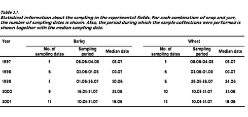
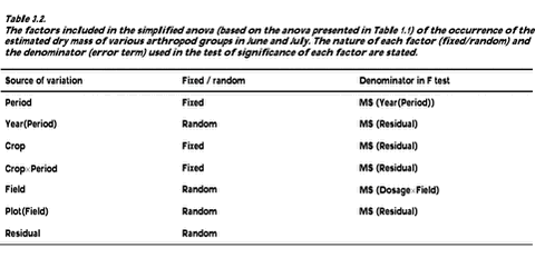
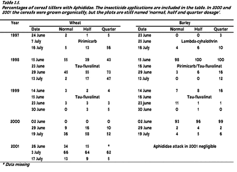
3 Arthropods (Navntoft, S. & Esbjerg, P.)3.1 Methods3.1.1 Data sampling 3.1.2 Statistical analyses 3.2 Results 3.2.1 Dry mass analyses 3.2.2 Density analyses 3.2.3 Aphididae 3.2.4 Arthropods in relation to vegetation 3.3 Discussion The main purpose of the arthropod studies was to identify and quantify changes of the arthropod fauna occurring during conversion from conventional to organic farming, specifically for species being important prey items of birds and as natural enemies of crop pests. The hypothesis was that the arthropod abundance generally would increase as a consequence of conversion, primarily as a result of no pesticide applications. Carry-over effects from the differentiated pesticide input during the conventional phase (normal, half and quarter dosage of herbicides and insecticides) were seen as a weak possibility hampered by high mobility of many species. 3.1 Methods3.1.1 Data samplingSuction sampling with a large-scale suction sampler was used throughout the experimental period as the predominant sampling method. The sampler was mounted on a small trailer with a 4WD vehicle as traction (Navntoft & Esbjerg 2002). Sampling was restricted to the main crop area excluding the plot margins (minimum 20 m) to reduce interference between plots and edge effects. Within each plot, 15 sub-plots (sub-plot: ±10 m from a marker stick) were selected in which sampling was carried out. The 15 sub-plots were evenly distributed along 3 tramlines to which the sampling machinery had to stay in order to minimise crop damage. Consequently the length of the suction tubes limited sampling to within 1.5 meters from the tracks. Sampling was only carried out in dry weather and the sampling of a particular field was always finished within 1 - 1.5 hour between 10.00h and 21.00h. Each sample comprised 10 sub-samples of 10 seconds application of the vac-nozzle (total area 0.2 m2). The samples were immediately labelled and placed into cooling bags and then, later the same day, frozen. Sampling was carried out in June, July and early August during the conventional period and in May, June and July during the organic period (Table 3.1). If possible sampling was conducted just before insecticide applications and no samples were taken until about one week after spraying. After defrosting the samples were sieved through three grids (2.0, 1.4 and 1.0 mm laboratory test sieves, Endecotts Ltd. London) to extract animals from soil and debris. The arthropods were hand-picked from the grids and transferred to 70% alcohol. All arthropods, except Aphididae and Collembola found within the three grids, were collected. Animals passing through all grids were ignored because they were not important as Skylark prey (Chapter 5). The sample content was subsequently identified under binocular microscopes at 5 - 40 x magnification. The arthropods were identified at minimum to order, but preferable to more detailed taxonomic levels. Collembola were not included because they require a comprehensive soil-sampling program. Aphididae attacks were estimated by counting cereal tillers with Aphididae. On each assessment and in each plot, 100 randomly selected wheat and barley tillers on a diagonal transect (Danielsen 1992) were inspected and the number of tillers with Aphididae was counted. 3.1.2 Statistical analysesThe variables ’dry mass’ and ’density’ were used to analyse for transition effects of the conversion from conventional to organic farming. 3.1.2.1 Dry mass analyses The selection of arthropods included in the group ’Skylark prey’ was based on the frequency of occurrence in faecal Skylark pellets collected in the experimental fields in 2000 and 2001 (Chapter 5, Table 5.1). Arthropod dry mass was estimated from the formula W = 0.0305 × L2.62 mg, where L is the length of the arthropod in mm (Rogers et al 1977). The arthropod lengths used were obtained from the literature if the individual was identified to species and otherwise estimated by measuring between 50 to 100 randomly selected individuals (Navntoft & Esbjerg 2002). Because suction sampling did not start until early June in the period before conversion to organic farming (late May in 1999), and ended late July after conversion (Table 3.1), only data from June and July were included in the analyses. The experimental unit was a plot, each of which was represented by 15 samples per sampling date. The 15 samples were summarised and divided by three to form the dependent variable ’mg dry mass m-2’. Thereafter the data were loge(x+1) transformed to improve approcimation to a normal distribution. The data sampling can be classified as repeated sampling (Stryhn 1996), which may violate the required independence of data. To avoid this a geometric mean of the loge(e+1) transformed data accross the sampling dates in June and July was used for the analyses, leaving only one figure per combination of year (5), crop (2) and dosage plot (3) (n = 30). General Linear Models (GLM procedure in SAS/STAT) (SAS Institute 1990b) were used for the analyses of dry mass. As starting point the anova design shown in Table 1.1 was applied, and stepwise model reduction was used to reach the final model. If no significant dosage effect or any interaction including dosage could be found, the basic model was simplified by replacing the fixed dosage effect by a random plot effect (Table 3.2). Pairwise tests between specific groups were carried out using a Tukey-Kramer adjustment for multiple comparisons of least-squares means. In order to provide information about the development in available Skylark prey and arthropods in general during June and July, 2nd degree models were calculated using the REG procedure in SAS/STAT and presented in figures for both barley and wheat. As stated above only the differences between means, corresponding to the 0-degree models, were tested using the GLM-procedure, due to the high population-fluctuations of arthropods within and between years. Therefore, the 2nd degree models can only be considered descriptive and no final conclusions should be drawn from the models. 3.1.2.2 Density analyses To describe how the population of Aphididae specific predators (Coccinellidae, Syrphidae and Chrysopidae) developed during June and July, descriptive 2nd degree models were calculated and presented in figures. The method used is described above. 3.1.2.3 Arthropods in relation to vegetation Dry mass analyses The experimental unit was a plot and the dependent variable ’arthropod dry mass m-2’ (Skylark prey, Carabidae and Staphylinidae, all arthropods) was analysed in relation to the factors presented in Table 3.3. Only arthropod data from June and July were used to make the analyses comparable with analyses comprising the entire experimental period (cf. section 3.1.2.1) Because dry mass data of vegetation was only available after conversion the factor ’period’ could not be estimated. Furthermore, because of confounding it was not possible to include ’field’ and ’plot’ in the model (see Table 3.2). Also ’dosage’ was excluded because the factor generally proved to be insignificant for the Arthropods (section 3.2). The last component ’vegetation covariate×crop’ (Table 3.3) was included to test for a possible different regression coefficient for each crop. Three different covariates were used to describe the vegetation: 1. Cereal biomass, as the dominating biomass. 2. Biomass of dicotyledonous weeds, because of its importance to herbivorous insects important as Skylark Prey (Moreby & Sotherton 1997). 3. Biomass of all vegetation beneath the cereals, which, except serving as a food resource, may provide refuges and improve the microclimatic conditions for arthropods living on the crop floor (Burn 1989). Except for the cereal biomass the covariates were loge-transformed. To avoid problems with multicollinearity only one vegetation covariate was entered into the analyses at a time. Stepwise model reduction was used, with p > 0.0167 as removal criterion. The P-value of the removal criterion was adjusted by Bonferroni correction to estimate the correct level of significance (α‘ = 0.05/n = 0.05/3 = 0.0167, with n being the number of covariates tested).
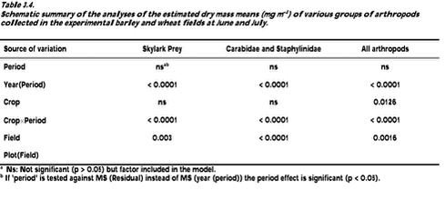
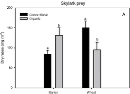
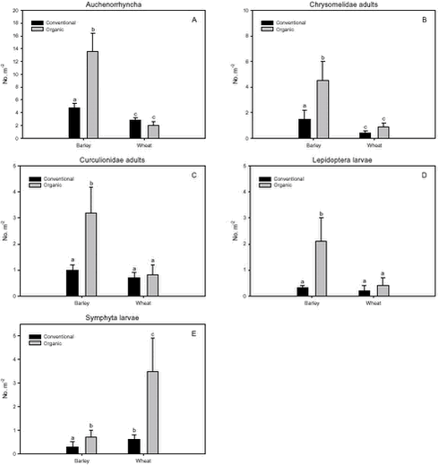
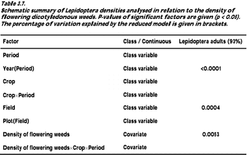
Density analyses The procedure was as described in the above section, except that in this case the basic model was the model presented in Table 3.2 in order to include the effect of ’period’. This model was extended with a ’weed covariate’ and a ’weed covariate×crop×period’. The last component was included to test for separate regression coefficients depending on ’crop’ and ’period’. Stepwise model reduction was used and after Bonferroni correction the removal criterion was p = 0.05/2 = 0.025, because two covariates were tested. Emphasis was put on the dominating herbivore groups foraging on weeds. The groups were: 1. Auchenorrhyncha, 2. Chrysomelidae, 3. Curculionidae and 4. Lepidoptera . The abundant herbivore group Symphyta was dominated by species also foraging on the cereal crop, and the group was therefore not expected to be correlated to the weed. To test for more specific host plant – herbivore relationships, the density of Auchenorrhyncha was analysed in relation to the density of monocotyledonous weeds. Furthermore the density of Polygonum aviculare and Bilderdykia convolvulus was tested in relation to Gastrophysa polygoni and the density of Cruciferae was tested in relation to Ceutorhynchus. The density of flowering plants is known to be a limiting factor for insects feeding on nectar and pollen (Altieri & Whitcomb 1979). To elucidate such a relationship, the density of flowering dicotyledonous weeds (cf. chapter 2) was analysed in relation to the density of Lepidoptera adults. Data of flowering weeds from 1997 were lacking and this year was consequently not included in the analysis. The specific tests were carried out as described above. 3.2 Results3.2.1 Dry mass analysesNo significant ’dosage’ effects were found and consequently the data were analysed by the simplified anova design (Table 3.2). Furthermore, no significant ’period’ effect across crops of the three arthropod groups analysed was found (Table 3.4), but for all groups there were clearly significant effects of ’year(period)’ (p < 0.0001) and ’cropXperiod’ (p < 0.0001). The interactions indicate that a difference between the two periods exists, but the effect varies between years and crops. Pairwise t-tests (Tukey-Kramer adjusted for multiple comparisons) on the interaction ’cropxperiod’ revealed a significantly higher Skylark prey biomass in barley after conversion to organic farming than the period before (p = 0.0002). Contrary, in wheat a significantly lower Skylark prey mass was found for the period after conversion (p = 0.001) (Fig. 3.1.A).
A pairwise test on the dry mass of Carabidae and Staphylinidae revealed a significant decline in wheat after transition to organic farming (p < 0.0001) (Fig. 3.1.B), which also explains the decline in the Skylark prey in wheat after conversion, because the beetles constitute a significant part of the Skylark prey.
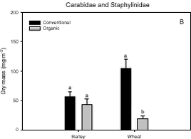
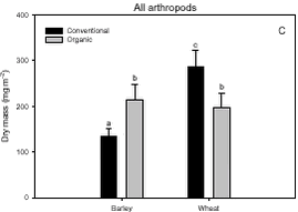
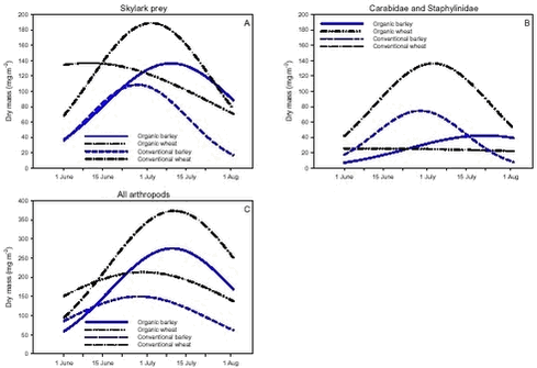
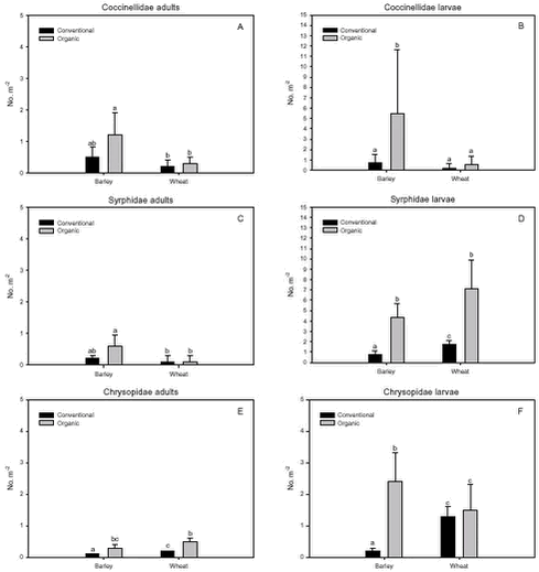
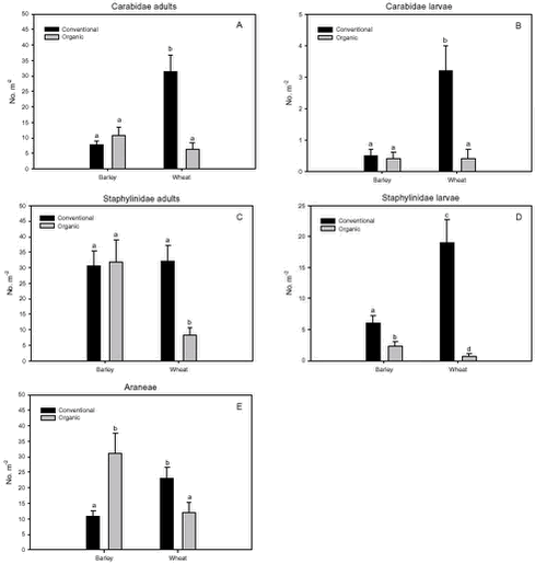
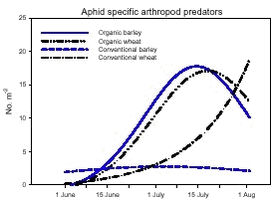
Fig. 3.1. Least-squares estimates and 95% CL of the ’year(period)’ factor for the dry masses of Carabidae and Staphylinidae were: 1997 = 48 (40-57) mg m-2, 1998 = 130 (108-156) mg m-2, 1999 = 74 (62-89) mg m-2, 2000 = 41 (34–48) mg m-2 and 2001 = 20 (17-25) mg m-2. The estimates of both years after conversion were lower compared to conventional growing, especially in 2001. Wheat was grown on the same field (field 2, cf. appendix B) both years after conversion. In order to clarify the significant effect of ’field’ on the Carabidae and Staphylinidae, least squares estimates and 95% CL are given: Field 1 = 33 (28-39) mg m-2, field 2 = 67 (57-78) mg m-2 and field 3 = 48 (40-57) mg m-2. For the total dry mass a significant increase was found after conversion in barley (p = 0.0002), but a reverse effect was found in wheat (p = 0.0022) (Fig. 3.1.C). In Fig. 3.2 descriptive models indicate the development over time (June and July) of the dry mass of Skylark prey, the dry mass of Carabidae and Staphylinidae and the total arthropod dry mass are presented. The dry masses of Skylark prey and all arthropods apparently started higher in organically grown wheat than in conventional wheat; Skylark prey about twice as high. When the season developed, however, the estimated dry masses in conventional wheat exceeded the corresponding amount in organic wheat mainly due to a stronger contribution of carabids and rove beetles. In barley, the models indicate that the dry masses of Skylark prey and all arthropods generally were higher in organic than in conventional barley, except at the beginning of the period were they tended to be at a lower level because of a higher dry mass of Carabidae and Staphylinidae in conventional barley. Fig. 3.2. 3.2.2 Density analysesIn this section the focus is put on herbivores important as Skylark prey, Aphididae specific predators as well as a couple of important generalist predators. No significant effects of previous spraying intensity were revealed (no ’dosage’ effect or interactions including ’dosage’). Furthermore, no general ’period’ effect could be revealed across crops of the various population analyses. For all tested populations, however, a significant ’period×crop’ effect was found (p < 0.05), indicating that a difference between the two periods exists, but that the effect varied between the two crops. Pairwise t-tests (Tukey-Kramer adjusted for multiple comparisons) on five groups of herbivores important as Skylark prey and 11 groups of important predators, Aphididae specific and generalists, on the interaction ’crop×period’ are presented in Figs. 3.3, 3.4 and 3.5. As seen from Fig. 3.3 the clearest effects on herbivores of conversion to organic farming were found in barley, in which all five tested groups occurred in significantly higher numbers after conversion. Contrary, in wheat only the density of Symphyta larvae were significantly higher after conversion, considerably higher than in barley. Fig. 3.3. The juvenile stages of the Aphididae specific predators in barley: Coccinellidae, Syrphidae and Chrysopidae benefited most of organic farming, with significantly higher density after conversion (Figs. 3.4.B, 3.4.D and 3.4.F). Generally, the trend of the Aphididae specific predators was higher abundance in the organically grown cereals (Fig. 3.4). Fig. 3.4. For the generalist groups Carabidae, Staphylinidae and Araneae, a significant decrease in the numbers of adult Carabidae and larval Carabidae was found in wheat after conversion to organic farming (Figs. 3.5.A and 3.5.B). The total catch of the adult Carabidae was dominated by Trechus spp. (74%) and Bembidion spp. (17%). Also the density of adult Staphylinidae decreased significantly in wheat after conversion but the density of Staphylinidae larvae diminished in both barley and wheat at organic growing (Figs. 3.5.C and 3.5.D). Furthermore, a significant increase in the density of Araneae was found in barley, but contrary there was a decrease in abundance of Araneae in wheat (Fig. 3.5.E). Fig. 3.5. In Fig. 3.6 the development during the season of the total number of Aphididae specific predators is indicated. The total population in conventional barley never seems to reach any size of importance, whereas the population of predators in conventional wheat peaks at the end of the period; about 14 days later than in organic wheat. The development in organic barley and organic wheat are quite similar. A steeper population build-up is indicated in June and the first half of July compared to the conventional cereals, and both populations peak in the middle of July; in barley about one week earlier than in wheat.
Fig. 3.6. 3.2.3 AphididaeThe estimates of Aphididae attacks are presented in Table 3.5. In wheat the dominating Aphididae was Sitobion avenae and in barley Rhopalosiphum padi.
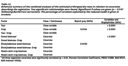
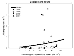
3.2.4 Arthropods in relation to vegetation3.2.4.1 Dry mass analyses Significantly positive relationships were revealed only between ’dicotyledonous weed biomass’ and ’Skylark prey’ as well as between ’Cereal biomass’ and ’Carabidae and Staphylinidae’ (Table 3.6). The corresponding models based on parameter estimates of the significant factors are illustrated in Fig. 3.7.
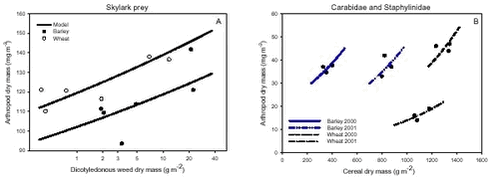
Considering ’Skylark prey’, 45% of the explained variation between plots came from differences between the ’crops’ and 55% from differences between the ’dicotyledonous weed biomass’. Regarding ’Carabidae and Staphylinidae’, 41% of the explained variation was due to differences between ’years’, 33% due to ’crop’ differences and 26% because of variation in the ’cereal biomass’. Fig. 3.7.Models of the relationships between estimated vegetation dry mass and arthropod dry mass at organic farming. Notice that the model graphs do not show the range of variation and that the log-transformed dry masses are not comparable with normal arithmetic means. The high position of the wheat curve in Fig. A, which is in contrast to Fig. 3.1.A is due to the following: In Fig. 3.1.A the dry mass has been statistically adjusted for the effect of ’field’ while it was not possible to include this correction in the figure above because the effects of crop and field were confounded. 3.2.4.2 Density analyses No significant relationships were obtained between the two general covariates density and diversity of weeds and density of herbivorous arthropods. Neither were any significant relationships revealed from the specific host plant – herbivore analyses. However, a significant relationship was found between the density of flowering weeds and Lepidoptera adults (Table 3.7). The corresponding model based on the parameter estimates of the significant factors is illustrated in Fig. 3.8.
Of the explained variation the covariate of flowering weeds only accounted for 6%. For the class variables 33% of the variation came from ’period’ (although not significant), 44% from ’year(period)’ and 16% from ’field’.
Fig. 3.8. 3.3 DiscussionIn a multi-trophic context the present arthropod studies identifies temporal trends in a variety of arthropod groups during conversion from conventional to organic farming analysed by means of dry mass and density estimates. In spring barley there was, in agreement with the working hypothesis, a clearly positive effect on the estimated Skylark prey dry mass and the total arthropod dry mass as a result of conversion to organic farming (Figs. 3.1.A and 3.1.C). Fig. 3.2 indicates that the difference was a result of higher estimated dry masses from the middle of June onwards at organic farming. Contrary, lower corresponding dry masses were found in winter wheat after conversion (Figs. 3.1.A and 3.1.C), mainly as consequence of a lower dry mass of Carabidae and Staphylinidae (Figs. 3.1.B and 3.2.B). Actually in wheat the estimated dry masses of Skylark prey and all arthropods were higher at organic farming in the first half of June. Afterwards, however, both dry masses in wheat at conventional farming exceeded the dry masses at organic farming (as indicated by Figs. 3.2.A and 3.2.C) due to a higher contribution of the epigaeic beetles (as indicated by Fig. 3.2.B). Before conversion to organic farming, Carabidae and Staphylinidae constituted 68% of the estimated dry mass of Skylark prey in barley and 70% in wheat. After conversion these shares declined to 33% in barley and 20% in wheat (Fig. 3.1). In barley this was mainly due to a higher abundance of the other arthropod groups, which were part of the Skylark prey (Figs. 3.3, 3.4.D and 3.4.F). In wheat the effect was a result of reduced abundance of the polyphagous predators (Fig. 3.5) and a higher abundance of the other Skylark prey groups. Only two of the groups presented in Figs. 3.3 – 3.5 benefited, however, significantly from organic farming in wheat. This was Symphyta larvae (Fig. 3.3.E) and Syrphidae larvae (Fig. 3.4.D), which both were part of the Skylark prey. Wheat was grown in the same field both years after conversion to organic farming, and the statistical effect of ’field’ was therefore especially in wheat an important factor. Least squares estimates of the dry mass of Carabidae and Staphylinidae in the three fields revealed that the lower abundance of the epigaeic beetles was not due to a generally lower occurrence in field 2 (section 3.2.1). It should also be noticed that the actual observations of the estimated Skylark prey in organic wheat actually was higher than in organic barley (Fig. 3.7.A). However, when comparing the conventional and organic periods there are statistically adjusted for differences between fields. Therefore the estimated dry mass means for organic wheat becomes lower than for organic barley (Fig. 3.1.A). Still, if the field factor is excluded from the models (although significantly) the estimated dry masses of organic wheat do no exceed conventional wheat. There was a tendency towards higher populations of Aphididae specific predatory insects in the organically grown period, especially of juvenile stages in barley (Figs. 3.4 and 3.6). Contrary, Fig. 3.6 indicates that the population of Aphididae specific predators in conventional barley never managed to build maybe because of lethal effects of insecticide applications and indirectly because of food shortage. The dominating Aphididae species in barley was the early occurring R. padi. That species never occurred in high numbers during the second half of the sampling season (Table 3.5), thereby providing no food for the predators. In conventional wheat, the reason for the late peak in the population of Aphididae specific predators could be, that the predators were able to recover from the insecticide applications. This was probably because the dominating Aphididae species, S. avenae, occurred later in the season compared to R. padi despite insecticide applications (Table 3.5). Due to the very distinct differences of the infestation level it is difficult to reach any conclusion regarding conversion effects on Aphididae. However, the heavy infestation in barley early in 2000 resulted in yield loss (M. Tved pers. comm.). Contrary, the infestation in barley in 2001 was negligible. Insecticides may have a major impact on the observed differences in arthropod abundance between the two farming regimes. A possible reason for the pronounced effect found on herbivores in barley compared to wheat is that the arthropod fauna may have been depressed more by insecticides in barley than in wheat. That was because of the more open structure in barley, allowing insecticides to penetrate deeper into the canopy. The two groups, which occurred in significantly higher numbers in organic wheat, Symphyta and Syrphidae larvae, are both highly sensitive to insecticides (e.g. Sotherton 1990, Hassan et al. 1987), which may explain the increased density at organic growing. However, Moreby & Sotherton (1997) stated that weed diversity and density and other less obvious factors including crop variety, crop rotation, past history of pesticide use, cultivation techniques, fertilizer type and level could all have an effect. No effect of the previous pesticide dosage level was found on the arthropods. Even before conversion to organic farming there was no significant effect of dosage on the arthropod abundance. However, if a dosage effect was found in the conventional phase, it is doubtful if a carry-over effect could have been revealed after conversion. That is because most of the field inhabiting arthropods are very mobile and therefore overshadow effects of previous treatments. Higher weed populations in the reduced dosage plots, however, could have lead to an indirect carry-over effect due to a higher supply of host plants but that was not the situation. The lower abundance of Carabidae observed in winter wheat in this experiment is in agreement with findings by Moreby & Sotherton (1997) based on D-vac samples. They also found that Carabidae tended to be more numerous on the conventional fields compared to the organic fields, which have been pesticide-free for at least two years. As was the case in this experiment Moreby & Sotherton (1997) found, that significantly higher densities did occur in the organic winter wheat fields for some of the “chick-food” insect groups, but generally the number of individuals were similar in both farming regimes. Moreby & Sotherton (1997) found that a greater diversity of broad-leaved weed species might have influenced the abundance of “chick-food” insects positively in organic fields by the provision of host plants for phytophagous species of Chrysomelidae, Lepidoptera, Heteroptera and Tenthredinidae. In line with this, the present study revealed a significant positive relationship between the dry mass of dicotyledonous weeds and dry mass of Skylark prey (Fig. 3.7.A). It should, however, be stated that the analysis is based on few observations, raising questions about the validity of the model. The effect indicated could be due to a combination of improved food availability for herbivores and a more favourable microclimate. Dry mass data of weeds, however, was only available after conversion to organic farming (cf. chapter 2). It is therefore not possible to validate if the relationship can explain the conversion effects on the arthropod fauna. A significant relationship was also revealed between the cereal dry mass and the dry mass of Carabidae and Staphylinidae (Fig. 3.7.B); again only for the period after conversion. However, the combination of few observations and a large variation between years (Table 3.6) leads to that no straight foreward can be made. Although no data are available on the crop dry mass at conventional farming, the yield data are given (appendix B). If assuming that yield is positively correlated with dry mass, the dry masses of both wheat and barley are markedly lower after conversion to organic farming. This supports the relationship since lower dry masses of Carabidae and Staphylinidae were observed after conversion, although only significantly in wheat (Fig. 3.1.B). It is doubtful if this correlation alone can explain the diminished abundance of the epigaeic beetles at organic growing. Other factors like weed hoeing may also be important (see below). The relationship, however, between crop biomass and the epigaeic beetles is supported by results of Krooss & Schaefer (1998). They found that because of high weed cover under extensive cropping of winter wheat (no fertilizer, no pesticides but mechanical weed hoeing), high species richness and high population density of Staphylinidae should be expected. However, the opposite effect was found (as in this study). Species richness was poor and fewer beetles were caught compared to other cropping systems. The lack of fertilization reduced the number of wheat plants per square-meter and the remaining stalks were much thinner. Consequently, the yield decreased to 50% compared to conventional farming (in our study the decrease was about 40%). The weed cover could not compensate for the change of microclimate because of the sparseness of the crop. Hence, accordingly to Kroos & Schaefer (1998), unfavourable microclimatic conditions may have caused low population density at extensive farming. No significant relationships could be revealed between the density and diversity of weeds and the density of important herbivores (section 3.2.4.2). The reasons could be several. Only in wheat a higher weed density was observed after conversion (cf. chapter 2). Contrary the least effects of conversion on herbivores were found in wheat. A possible reason is, that the occurrence of weeds was too low to support measurable population changes. Even at low levels, organic barley had a ten times higher weed biomass than organic wheat (cf. chapter 2). This was reflected on the abundance of herbivores, which, for the four dominating herbivore groups dependant on weed, Auchenorrhyncha, Chrysomelidae, Curculionidae and Lepidoptera, was several times higher in organic barley that in organic wheat (Fig. 3.3). Furthermore the weed diversity generally did not increase as a result of conversion (cf. chapter 2) and it could therefore not explain the conversion effects on the arthropods. Of the more specific host plants included in the analyses the density of Brassicaceae increased significantly in both crops after conversion as did the density of P. aviculare and B. convolvulus in wheat (cf. chapter 2). However, according to the combined analyses those increases did not lead to higher densities of related insects, at least not within the time frame of this project. Even though weed density and diversity may not be complete measures of the flora, it leaves an impression that the insecticides had a larger impact than the weed flora for the conversion effects observed on the arthropods. The weed density in the present study was low even after conversion (cf. chapter 2) and a successful weed control at organic farming may explain the lack of positive relationships. However, the higher number of flowering dicotyledonous weeds at organic farming (chapter 2) apparently did affect the pollinating and nectar feeding insects right after conversion, exemplified by the positive relationship with Lepidoptera adults (Fig. 3.8). Conclusions based on this model, however, should also be treated with caution because the factor ’density of flowering dicotyledonous weed’ only accounted for 6% of the explained variation. It is questionable whether the catch crops affected the arthropod fauna during the sampling season. When present the catch crop mostly constituted only a fraction of the already low weed biomass (cf. chapter 2). However, naturally the growth picks up as the cereals mature. It is therefore possible that the impact of the undersown crops on the arthropods increases towards the end of the sampling season. Otherwise its significance can not be expected until after harvest. It is possible that the ongoing weed hoeing at organic farming generally has a negative impact on ground/soil dwelling species. This may be particularly apparent for winter wheat in which no tilling operations normally are carried out in the spring at conventional growing. Reasons for the pronounced negative effect on the epigaeic beetles especially in wheat may therefore be disturbance and changed microclimate. Lorenz (1994), however, found no negative response of Araneae, Carabidae or Staphylinidae to mechanical weed control. His results, though, were obtained in sugar beets. Beets already harbour low densities of epigaeic beetles (Navntoft & Esbjerg 2002), a fact which probably makes it difficult to detect an effect. Contrary Holm et al. (unpubl.) found, that it may generally be assumed that soil-tilling has a negative impact on arthropods. Furthermore, Fadl et al. (1996) found that catches maid during the main emergence phase of the new generation of the carabid Pterostichus melanarius were lower in spring-cultivated fields compared to uncultivated or autumn fields. Apparently the reason was reduced larval/pupal survival because of the spring soil cultivation. Weed hoeing may also result in food depletion for the ground dwelling predators and thereby indirectly suppress the populations. Weed hoeing may e.g. reduce the density of Collembola. These soil-inhabiting arthropods are an important prey group for generalist predators (Sunderland 1975) and the hygrophilic species are generally vulnerable to desiccation (Sjursen et al. 2001), which most likely follow mechanical weed hoeing. The results in our experiment, however, may be biased by the more ’gentle’ suction it was necessary to perform in the organic wheat, because large amounts of soil accumulated in the collecting jars as a consequence of the weed hoeing. In conventional wheat a hard shell was created on top of the soil, which made it possible to suction sample more intensively at the soil surface level. Furthermore, suction sampling often underestimate nocturnal species, which include most of the carabids found in agricultural habitats (Thiele 1977). Especially populations of larger species may be underestimated.
|