| Front page | | Contents | | Previous | | Next |

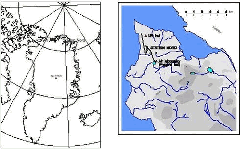
AMAP Greenland and the Faroe Islands 1997-2001

1 Atmospheric environment

Citation: Christensen, J. H., M. Goodsite, N. Z. Heidam, H. Skov & P. Wåhlin: Chapter 1. Atmospheric Environment. In: Riget, F., J. Christensen & P. Johansen (eds). AMAP Greenland and the Faroe Islands 1997-2001 Vol. 2: The Environment of Greenland. Ministry of Environment, Denmark Department of Atmospheric Environment, National Environmental Research Institute, Frederiksborgvej 399, Box 358, DK-4000 Roskilde, Denmark

1.1 Introduction

The atmospheric AMAP Assessment presented below is based on the results from the Danish programme for the Arctic atmosphere, which has been carried out in North Greenland as an interacting combination of field measurements of air pollutant concentrations and model calculations of air pollution transport in the Northern Hemisphere.

The monitoring programme and some selected results are presented in section 1.2. The model system is described in section 1.3, which also holds comparisons between measured and calculated air concentrations. This chapter also presents calculated atmospheric depositions for several pollutants at various locations in Greenland, split into quantified contributions from different and geographically distant source areas. Mercury deposition estimates for the Northern Hemisphere are also presented. In section 1.4 measurement and model data from the period since 1990 are successfully combined to demonstrate that ambient air concentrations in northeastern Greenland have decreased during the last decade. Quantified trends, attributable to emission reductions in distant source areas, are presented for several pollutants.

1.2 Atmospheric Monitoring

1.2.1 Location and instrumentation

The Danish atmospheric monitoring programme has been carried out by the Department of Atmospheric Environment (ATMI) at the National Environmental Research Institute (DMU) since 1990, and as an official AMAP programme since 1994. The monitoring has taken place at Station Nord, a small military air field located in north-eastern Greenland at 81⁰36‘ N, 16⁰40‘W, see Figure 1.2.1 (left). The measurements started at the site named ’LW hut’ on the map but have since 1995 been performed at the site ’Flyger’s Hut’, which is located approximately 3 km south of the central complex of buildings, as shown on the map in the Figure 1.2.1 (right). The building is supplied with electricity and heat and serves as the main base for the AMAP Air Monitoring Programme. The location of the AMAP station has been chosen so as to minimise influence from any local air pollution.

The instrumentation at this site consists of a filterpack-sampler operated on a weekly basis. The sampler consists of a sequence of 3 - 4 filters of which the first collects particles. The subsequent filters are specially impregnated to collect various gases, notably SO₂. The particle filters are analysed for the sulphate-, ammonium- and nitrate- ions, SO₄^2-, NH₄ + and NO₃ - and, by the PIXE method, for a substantial number of elements including several heavy metals. The gas filters also collect ammonia (if any) and nitric acid, NH₃ and HNO₃ but since the particle phases of these nitrogen components may de-gas from the first filter onto the gas filters only the total sums of particulate and gaseous phases are reported for these nitrogen compounds.

Monitors have been used to carry out measurements with high time resolutions for ozone since 1995 and for gaseous elementary mercury since 1999 where a monitor has been operated from early winter until autumn.

The personnel at Station Nord carry out the daily supervision of the instruments. They also handle all new filters and return exposed samples together with the experimental protocol and diskettes with ozone and mercury data to DMU utilising all available flights.
Maintenance and calibration of the instruments at the field sites have been carried out regularly by the staff from DMU, usually in late winter and in late summer or early autumn/winter. The field visits have also been very useful for exchange of information and experience on instrument field performance between the laboratory staff and the station personnel. At these visits the monitors have usually been taken home for maintenance and substituted with freshly serviced instruments. The quality of measurements with monitors is regularly controlled (at least weekly) by adding standard to the sample inlet.

Figure 1.2.
Greenland with the location of Station Nord (left) and the position of the air monitoring site at Station Nord. The regular AMAP site is located at Flygers‘ hut (right).

1.2.2 Gas and aerosol measurements

The measured concentrations of a number of pollutants are shown for the period 1990 - 2001 in Figures 1.2.2 and 1.2.3. In Figure 1.2.2a the gaseousSO₂ is shown on top of the shaded particulate SO₄ 2- and selected nitrogen compounds are shown in Figure 1.2.2b and 1.2.2c. The persistent patterns of high concentrations in winter and early spring and very low concentrations in summer, described previously (Christensen et al. 2000, 2001) are clearly to be seen for all pollutants. For sulphur in particular the maximum weekly average concentrations in the remote north-eastern Greenland are comparable to the annual mean values around 1.5 mg S/m³ found in rural districts of Denmark.

These recurrent annual cycles from low to high concentrations, separated by 2 decades of magnitude, are ascribed to the seasonal atmospheric circulation patterns characteristic of the High Arctic. In winter the circulation often favours transport into the Arctic from mid-latitudinal regions with prominent pollution sources. In summer, on the other hand, the circulation in the Arctic atmosphere is essentially local and confined within the region with its few and small emissions so the concentrations fall to very low values.

 
Figure 1.2 a, b, c.
Weekly average concentrations through the 1990s of sulphur and nitrogen components. Total concentratio ns (phase sums) in figs. a and c  are shown as red dots, and the particulate phases in figs. a and b  as blue crosses – overlaid by smoothing curves.

The patterns of the gaseous and particulate phases of sulphur differ in that the high concentrations of SO₂ appear episodically early in winter, in contrast to the slower but consistent build-up of particulate bound SO₄^2- that starts somewhat later.

These patterns are probably related to the different atmospheric characteristics of the two pollutants. The occurrence of the primary pollutant SO₂ is presumably controlled by meteorological switching between periods of atmospheric transport headed directly at north-east Greenland and periods where the transport is directed elsewhere. The concentration of the secondary SO₄ 2- depends of course also on transport from source regions, but more indirectly since it is produced from SO₂ wherever it occurs by fairly slow chemical oxidation processes. These processes are induced and enhanced by increasing solar irradiation but do require time to take effect. This secondary pollutant may therefore be more widespread and, also because of its longer lifetime in the atmosphere, it may arrive at the measuring point from a broader range of directions, hence the delayed and less episodic appearance of SO₄^2-

Figure 1.2.
Weekly average concentrations through the 1990s of heavy metals in aerosols shown as blue crosses– overlaid by smoothing curves. 

1.2.3 Elements and heavy metals 

The aerosol sampling and measuring of elements at Station Nord by PIXE has now been performed almost continuously for more than 10 years (since August 1990). Both the technique of sampling and the technique of elemental analysis have remained unchanged during this long time period. The results cover the weekly concentrations of a considerable number of elements and this large amount of data can be used to get a better impression of the different sources and of the average yearly cycle of the elements.
The COPREM receptor model has been used to build a data model for the elemental concentrations in the period 1991-2001. All receptor models, including factor analysis, are based on the assumption that the original receptor site concentrations can be adequately explained by a linear combination of contributions from various relevant sources with fixed composition such that

(1.2.1)

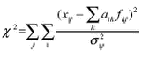
where x_ij is the measured ambient concentration of the pollutant i during sampling occasion j. A number of relevant sources k are considered significant. The coefficients a_ik represent the constant source profiles, and f_kj represent the strengths of the sources found in the individual samples. Factor analysis is a general method of simplifying the problem in equation 1.2.1 in which the only necessary input is the set of numbers x_ij. The analysis does not give a specific solution, but merely a less complex subspace with still an infinite number of different solutions.

The Constrained Physical Receptor Model (COPREM) relies on the same basic receptor model as factor analysis (equation 1.2.1). The equation is solved by an iterative method to determine the source strengths f_kj and the source profiles a_ik (Wåhlin, 1993). The chi-square statistic  

(1.2.2)

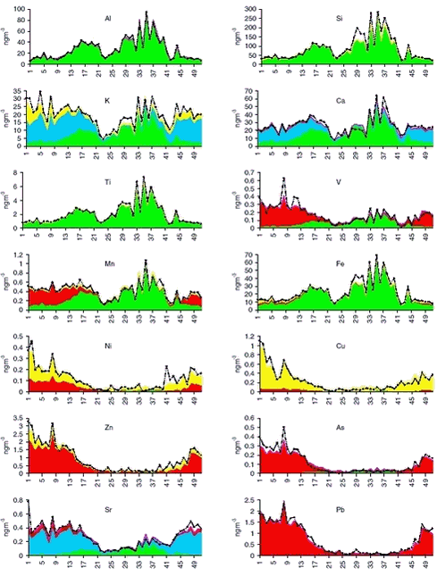
measures the total squared distance between the measurements and the model in units of the uncertainties of the data σ_ij.

Built-in model constraints exclude non-physical solutions (negative coefficients in the source profiles and negative source strengths), and additional constraints can by means of a form matrix be included to fix profile components in constant ratios, partly or entirely. The chi-square statistic is minimised within the limits imposed by constraints. An initial profile matrix is set up in which the source vectors have the main characteristics of known sources, and the form matrix is set up to maintain these characteristics, and to prevent the profiles from mixing together during the iteration. In this way any a priori knowledge about the character of the sources can be used to achieve a polarised solution as elements can be allowed to enter only in certain source profiles. The COPREM also take into account uncertainties, which is of particular importance for measurements near the detection limit. Chemical compounds, which do not fit into the simple linear model and therefore need special handling, are easily recognised.

At Station Nord the measured concentration data for all PIXE elements except S, Cl and Br can be expressed as combined contributions from only 4 sources. These comprise a crustal source (soil), a marine salt source (sea), a prominent anthropogenic source (combustion), and an additional anthropogenic source (metal) with contributions of the metallic elements Ni, Cu and Zn.

Local sources (i.e. anthropogenic emissions from Station Nord itself) are normally negligible. Only very few episodes of substantial local air pollution (caused by waste burning in the summer) has been noticed since the start of aerosol measurements at Station Nord in 1990.

All samples are week samples starting Monday 0:00 UTC and they can therefore be assigned a specific week number in the range 1-53 for every year. The average yearly variation of each element as a function of the week number was calculated by averaging concentrations with the same week number for all years. In this way, a lot of week-to-week scatter in the influx from the different sources is smoothed out, and the gross seasonal variation is more easily observed. The average annual variations of the concentrations of selected PIXE-elements at Station Nord in the years 1991-2001 is shown below in Figure 1.2.4 ordered by their atomic number. In this figure the results of COPREM receptor analysis on source contributions are also shown.

View the image in full size
Figure 1.2.
Annual elemental concentrations averaged over 1991 – 2001, as a function of week number. The source apportionments according to COPREM are shown for the four main sources. The colours indicate: Soil (green), sea spray (blue), combustion (red) and copper smelters (yellow).

Elements such as Al, Si, and Ti are of almost pure crustal origin, and it can be seen clearly that their seasonal variations are very much the same, and can be fitted with the same soil source time signal with peaks in spring and late summer.

The elements Fe, Mn, V, As and Pb are in this order under increasing influence of the combustion source compared to the soil source. The elements As and Pb in the lower right corner of the figure have almost the same seasonal variation showing the pure combustion time signal with peaks in the winter and almost total absence in the summer, which is typical for Arctic Haze. As described earlier the time signal for totalS is a little different, probably due to a longer lifetime of sulphur particles in the atmosphere compared with sulphur dioxide. Sulphur dioxide peaks in the winter, while sulphate/sulphuric acid peaks in the spring (after Polar Sunrise).

The elements Ca, K and Sr are abundant in seawater and in aerosols created by sea spray. The elements, which also have a crustal and a combustion origin, are in this order under increasing influence of the sea source. The sea signal has peaks in the winter half-year showing the influence at Station Nord of ocean storms.

The elements Zn, Ni and Cu have additional winter peaks not found in the common anthropogenic combustion signal. The deviations can be described by an additional anthropogenic source involving particularly high emissions of these metallic elements. The elements are in this order under increasing influence of the metal source.

1.2.4 Ozone and mercury measurements

Mercury is found at high levels in marine animals at many places in the Arctic and North Atlantic Ocean. It has been shown that the present levels of mercury in sea animals have a negative effect also on the health of the local populations, dependent on these animals as food supply (Grandjean et al. 1998).

The lifetime of atmospheric elemental mercury (GEM) (95% of atmospheric mercury) is in general about 1 year (Lin & Pehkonen, 1999). In the Arctic during spring, the lifetime of GEM is significant shorter and GEM is observed to be depleted in less than one day during mercury depletion episodes (MDE), (Schroeder et al. 1998, Lindberg et al. 2002, Skov et al. 2002). GEM is converted to oxidised mercury in the gas phase the socalled reactive gaseous mercury (RGM) that is fast deposited to the ground (Goodsite et al. 2002). Recently MDE’s have been observed also in Antarctic (Ebinghaus et al. 2002). MDE occurs at the time where the Arctic ecosystems are extremely active. Therefore it is hypothesised that there is a higher efficiency of bioaccumulation of mercury that would be expected from extrapolating data from mid-latitudes to Arctic and therefore it is very important to get a fully understanding of the processes leading to MDE’s. The improved knowledge of the concentrations, deposition and atmospheric processes in the Arctic is intended to lead to better performance of atmospheric chemical transport models and thereby an improved understanding of the source-receptor relationship for atmospheric mercury. At present it is not clear what the benefits are to improved ecosystem quality in the Arctic, if emission reduction strategies are proposed because of the lack of understanding of the processes controlling atmospheric mercury. Only improved model performance and confidence in the calculations will help in the decision making process.
Ozone has been observed to be depleted during spring for nearly ten years and it is well accepted that it is due to photochemical degradation after the polar sunrise. More recently it has been demonstrated that GEM is depleted as well and it is strongly correlated with ozone during MDE (Schroeder et al. 1998) and that the GEM depletion is triggered by solar radiation (Lindberg et al. 2002). However, very little is known about the reaction mechanisms. Several hypotheses have been proposed where Cl and/or Br atoms or ClO and/or BrO are common candidates. In this section, measurements of tropospheric mercury and ozone at Station Nord, Northeast Greenland are presented. The data are treated using basic reaction kinetic theory and physical theory for mixing of gases in the atmosphere.

1.2.4.1 Experimental

The analytical techniques for measuring ozone and GEM have been presented in a previous AMAP report, Christensen et al. (2001), and will only be described shortly here.

Ozone is measured with an UV absorption monitor, Monitorlab 8810, with a detection limit of 1 ppbv and an uncertainty of 3 % for concentrations above 10 ppbv and 6 % for concentrations below 10 ppbv, (all uncertainties are at a 95% confidence interval). GEM is measured by a TEKRAN 2537A mercury analyser where GEM is collected from the sample air on a gold trap from where mercury is thermally desorbed using argon as carrier gas and then analysed with cold vapour atomic fluorescence spectroscopy. The detection limit is 0.1 ng/m3 and the reproducibility for concentrations above 0.5 ng/m3 is within 20% on a 95% confidence interval. It is not at present possible to give the combined uncertainty, as the exact identity of the measured mercury is unknown though GEM is determined as the dominant compound

1.2.4.2 Results

The results of ozone and GEM measurements are shown in Figure 1.2.5. It is seen that ozone is rather stable from September/October until the end of February/beginning of March, then a highly perturbed period is occurring where ozone and GEM at about 40 ppb and 1.5 ng/m³, respectively, are depleted within hours to 0. They remain at 0 for up to several days until they suddenly rise again. In July the ozone concentration stabilises around a little above 20 ppbv for slowly increase to about about 40 ppbv in September/October.

Figure 1.2.
Ozone mixing ratios measured from 1999 to 2001 at Station Nord. Gem is measured in the period from 25. September 1999 to 23. August 2000 and again 14. February 2001 to 23. August 2001.

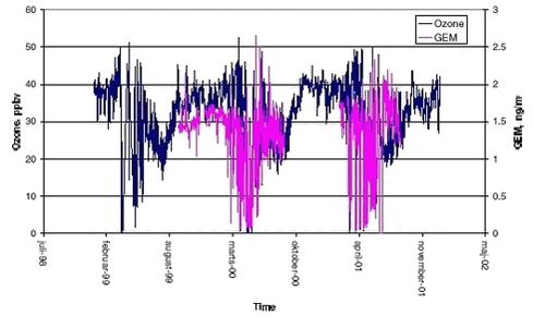
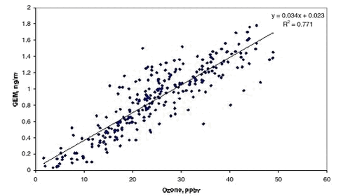
GEM was only measured from February to end of July or to the beginning of August. The measurements were focusing on the description of the highly perturbed period where ozone was depleted. Previously Schroeder et al. (1998) have described that ozone and GEM are highly correlated and this is indeed confirmed from the present data set, see Figure 1.2.6. Data was selected from periods where at least 3 consecutive concentrations were decreasing on both ozone and GEM and where the initial GEM concentration was above 0.4 ng/m³. After the depletion period some very high concentrations of GEM appeared with values up to above 2 ng/m³. Similar observations were also observed at Alert (Schroeder et al. 1999) and at Barrow (Lindberg et al. 2002) and they are attributed to reemission of mercury to the atmosphere. The interruption of the time series of GEM at Station Nord makes it difficult to further interpret if reemission is occurring at Station Nord.

A plot of GEM versus ozone at Station Nord is shown in Figure 1.2.6. There is a significant linear correlation (99.9 % significance level) between them. The slope is 0.034 ± 0.001 ng/m³/ppbv and the intercept is 0.023 ± 0.03 ng/m³. The slope is practically identical with the one obtained by Schroeder et al. (1998) at respectively 0.04 ng/m³/ppbv and 0.39 ng/m³ for the slope and the intercept confirming that it is the same process observed leading to MDE at Station Nord and at Alert, Canada.

Figure 1.2.
GEM against ozone concentrations at Station Nord including a regression line obtained by classical regression analysis.

1.2.4.3 Discussion
Reaction Kinetics

The interpretation of the correlation between ozone and GEM is not simple. The strong correlation indicates that ozone and GEM are dependent on a mutual factor. A direct reaction between ozone and GEM can be ruled out due to the long lifetime of GEM with respect to the present ozone concentrations. Hausmann & Platt et al. (1994) have shown that when ozone is decreased BrO is building up due to the reaction:


(1.2.3)

and therefore serious candidates for GEM removal are Br or BrO. However Cl and ClO cannot be ignored as significant Cl removal of organic compounds have been observed during MDE (e.g. Boudries & Bottenheim, 2000) and their importance depend on their reactivity towards GEM.

The lifetime of GEM is observed to be typically about 10 hours during MDE. Hausmann & Platt observed up to 20 pptv of ClO and BrO and thus the resulting rate constants for the reactions can be estimated to be in the order of 6x10^-14 cm³ molec^-1 sec^-1, which is reasonable.

BrO and/or ClO should then react with GEM

(1.2.4)

or

(1.2.5)

in competition with other reactions regenerating Cl and Br (ignoring heterogeneous reactions):

(1.2.6)¹

(1.2.7)²

If BrO is the main responsible for the GEM removal and we write the formation rate of Br from reaction 1.2.4, 1.2.6 and 1.2.7 and assuming steady state for the Br concentration the following equation can be deduced.

(1.2.8)

k_1.2.x is the reaction rate constant for reaction 1.2.x.

The part in parenthesis has to be negligible compared to k_1.2.4[Hg] in order to explain the strong linear correlation between ozone and GEM with a close to zero intercept observed in Figure 1.2.6. However both k_1.2.4 and k_1.2.5 are at least a factor 100 larger than k_1.2.4 (DeMore et al. 1997) and the concentrations of GEM, ClO and BrO are of the same magnitude, so the part in parenthesis is not negligible. The same considerations are valid if ClO is assumed to represent the main sink for GEM. Therefore the reactions of BrO and ClO with GEM most probably are of negligible importance.

The strong correlation observed in Figure 1.2.6 indicates that ozone and GEM is directly dependent on one another. Therefore the data was analysed assuming relative rate conditions between ozone and GEM. The method is widely used under laboratory conditions where the reaction of interest is running in competition with another reaction where the reaction rate constant is well established. So the system here is:

(1.2.9)

and

(1.2.10)

where X is either Br or Cl.

The kinetic equations for reaction 1.2.9 and 1.2.10 are:

(1.2.11)

and

(1.2.12),

respectively.

Dividing equation 1.2.11 with 1.2.12 the relative rate expression is obtained.

(1.2.13).

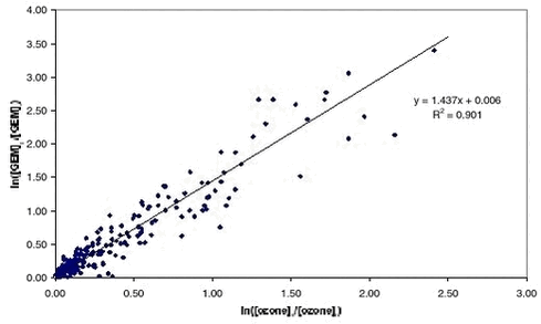
A plot of ln([GEM]₀/[GEM]_t against ln([O₃]0/[O₃]t should then give a straight line with intercept 0 and where the slope is equal to k_1.2.10/k_1.2.9. Figure 1.2.7 shows such a plot using the data from Station Nord where data has been selected for periods where the initial concentration of GEM was above 0.4 ng/m³ and where three consecutive measurements of both ozone and GEM are decreasing. All measurement included were for periods with 24 hour daylight.

Figure 1.2.
The natural logarithm to the relative concentrations of GEM and ozone during Depletion episodes in 2000 and 2001. The regression analysis is carried by orthogonal regression analysis. Only data are included where three consecutive measurements of both ozone and GEM are decreasing and where the initial concentration of GEM is larger than 0.4 n g/m³.

In fact there is a strong linear correlation (>99.9% significance). A straight line is obtained by orthogonal regression with intercept close to zero as expected from equation 1.2.13. The slope is 1.437 and significantly different from 1. A slope equal to one is expected if the correlation was only caused by dilution due to mixing of air masses. So first of all Figure 1.2.7 proves that ozone and GEM have a mutual dependence that cannot be explained solely by meteorology.

The rate constant of ozone with Br and Cl atoms is very well known due to their importance in the depletion of stratospheric ozone depletion (DeMore et al. 1997). Table 1.2.1 shows the calculated rate constants for GEM assuming respectively Cl reaction and Br reaction together. In the Table is also listed available data from the literature.


Table 1.2.
The calculated reaction rate constants for the reactions between GEM and Br and Cl based on Fig   re 1.2.7 and the reaction rate of Cl and Br with ozone from DeMore et al. 1997. The rate constants obtained in this study are calculated using a reaction rate for ozone at 233 K and 263 to be representative for the conditions in Arctic.

The reactions of halogens with Hg are independent of temperature (Horne et al. 1968, Grieg et al. 1970) and therefore results of the various studies should be directly comparable. The ozone reactions with halogen atoms are temperature dependent and the rate constants of Hg are calculated at 233 K and 263 K representative for the conditions in Arctic during mercury depletion. There are very few studies of the rate constant of Hg with Cl and Br. Horne et al. and Grieg et al. indicate that the results from their studies are correct within a factor 3.

In case of Br the reaction rate constant there is a factor 16 between the studies of Sommar et al. and Ariya et al. and the value obtained here is in between those values. Both groups used the relative rate technique in their study and more studies are needed in order to establish the correct reaction rate constant. For the reaction between Cl and Hg there appears to be an excellent agreement between the laboratory study of Ariya et al. and the results obtained in the field experiment.

In general the half-life of GEM at Station Nord is about 10 hours during MDE. Using rate constants of Ariya et al. (the largest values for the reaction rate constants) this corresponds to a concentration of either Br or Cl at 1 pptv and 0.1 pptv, respectively. Most laboratories report Cl concentrations in Arctic during MDE from 0.001 to 0.004 ppt (e.g. Boudries & Bottenheim, 2000, Röckmann et al. 1999, Jobson et al. 1994) at least a factor of 100 lower concentration than needed for the observed GEM depletion. Br in the ppt level is reported by many authors (e.g. Boudries & Bottenheim, 2000, Tuckermann et al. 1997, Jobson et al. 1994). Therefore it can be concluded that the direct reaction of Cl with GEM is not an important removal process during mercury depletion episodes but that Br is a serious candidate for the depletion.

Based on the results presented above the most important reactant for GEM removal is Br. However, there are still large uncertainties involved before a definitive answer can be given about the mechanisms of MDE’s. For example there is as previously mentioned a factor 14 difference between the results obtained in laboratory studies for the reaction of Hg with Br. To the knowledge of the authors there is not any study of the reaction rates constant of the reactions between Hg and ClO or BrO. The lack of temperature dependence and an eventual effect of pressure need to be documented as well.

1.2.4.4 Atmospheric implications

The measured GEM at Station Nord confirms atmospheric mercury as a global pollutant and that mercury depletion events (MDE’s) are phenomena connected to all coastal areas in Arctic during Arctic Spring. The MDE occurs in parallel with ozone depletion each spring in Arctic.

Strong indication for the reaction between Br and Hg as responsible for MDE’s in Arctic is found and therefore model calculation of atmospheric mercury has to include this reaction in the reaction scheme. Organobromides, sea ice and sea salt have been suggested to be sources of Br in the arctic troposphere. It is now generally accepted that releases from sea ice and sea spray are the main sources (Platt sand Moortgat, 1999 and references in there). Therefore model calculations of MDE should be restricted to air masses influence by marine air.

The reaction with Br with GEM leads to a monovalent mercury radical species. The further fate of this species is at present unknown but evidence is found for that it reacts further to form reactive gaseous mercury (Lindberg et al. 2002) which various divalent mercury compounds. The identity of RGM is at present unknown and it will be the future challenge of the scientific community to identify and describe the fate of RGM. How much is deposited to the snow surface and how much is reacting further for example with particles?

1.3 Atmospheric Modelling

A model is a mathematical tool for the study of processes and mechanisms of complex systems such as the atmosphere and the processes inside the atmosphere as f.ex. transport of air pollution. This tool should therefore take into account all processes, which the transports depend on. The air pollution in the Arctic depends on the emissions from the sources, transport from the emissions area into the Arctic by the wind, dispersion of the pollution by diffusion, chemical transformations during the transport, removal of pollutants due to precipitation and deposition on the surface. An air pollution model for the Arctic must take into account all these physical and chemical processes. The different processes must be described very precisely to reduce the uncertainties in the model. It is only possible to handle such a model on a very powerful computer, because the processes and the interactions between the different processes are very complex.

There are several reasons why one should use a model. A model is a good tool for improving the understanding of the atmospheric pathways to the Arctic. The model can also be used to trace the measured pollution back to different sources in the Northern Hemisphere and estimate their contributions to the Arctic atmospheric pollution, which is done in the following section 1.3.2. The model can also be used to quantify the importance of different processes as f.ex. mercury depletion for the transport of mercury into Arctic as shown in section 1.3.3. Finally the model can also be used for trend analysis of the measurements, e.g. by normalising the measurements for the meteorological factor, i.e. estimate the variations in the measurements that are due to changes in the meteorological conditions and then estimate the trend of the concentrations due to changes in the emissions. This is done in section 1.4.

The DEHM model has been used for this assessment. The DEHM model has earlier been used in AMAP phase 1 (see Kämäri et al., 1998), and the model has been described in several papers, see e.g. Christensen (1997, 1999), Barrie et al. (2001), Lohmann et al. (2001) and Roelofs et al. (2001). Model results from the Danish Eulerian Hemispheric Model will be presented in the following.

1.3.1 The DEHM modelling system

The system consists of two parts: a meteorological part based on the PSU/NCAR Mesoscale Model version 5 (MM5) modelling subsystem (see Grell et al, 1995) and an air pollution model part, the DEHM model (see Figure 1.3.1). The MM5 model produces the final meteorological input for the DEHM model. Global meteorological data, used as input to the MM5 mesoscale modelling system, are obtained from the European Centre for Medium-range Weather Forecasts (ECMWF) on a 2.5^ox2.5^o grid with a time resolution of 12 hours. The whole system includes 2-way nesting capabilities, so it is possible to do finer (150 km -> 50 km -> 16.67 km, etc) model calculations over e.g. the Arctic Ocean or Greenland. 23 years of meteorological data from 1979 to 2001 are available, but the MM5 model system for the mother domain has only been run for a period of 11 years from 1990 to 2001, while the model system with 1 nest has been run for the period 1995-2001 for Europe (50 km) and 1 month for Greenland (50 km) as demonstration.

In the version used here the model has been run for only the hemispheric domain.

Figure 1.3.1.
Overview of the DEHM model system.

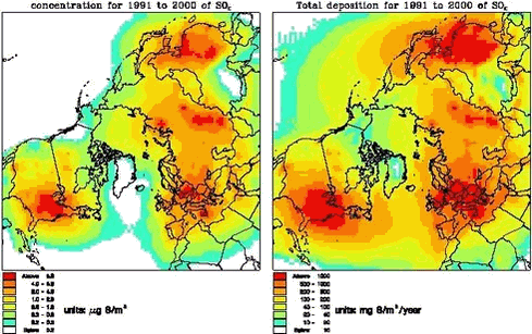
The DEHM model is based on set of coupled full three-dimensional advection-diffusion equations, one equation for each species. The horizontal mother domain of the model is defined on a regular 96x96 grid that covers most of the Northern Hemisphere with a grid resolution of 150 km x 150 km at 60^oN. The vertical discretization is defined on an irregular grid with 20 layers up to ≈ 15km that reflects the structure of the atmosphere.
The vertical diffusion is parameterised by using a K_z profile for the surface layer based on the Monin-Obukhov similarity theory, and this K_z profile for the surface layer is extended to the whole boundary layer by using a simple extrapolation (see Christensen, 1997).

1.3.2 Modeling of sulphur and lead

In the basic version the emissions of anthropogenic sulphur and lead are based on the global GEIA inventory of sulphur, version 1A.1, for 1985 (see Benkowitz et al., 1996) and the global GEIA inventory of lead, Version 1, for 1989 (see Pacyna et al, 1995), both on a 1^ox1^o grid. These emissions are redistributed to the grid used in the model. The EMEP emissions of sulphur (for Europe) for the years 1990-1997 are used for the part of the grid, which is equal to the EMEP grid.

The sulphur chemistry is simple linear, where the oxidation rate of SO₂ to SO₄^2- depends on the latitude and the time in the year, while for Lead there are no chemical transformations.

The dry deposition velocities of the species are based on the resistance method. The wet deposition is parameterized by using a simple scavenging ratio formulation with different in-cloud and below-cloud scavenging. The removal rates for Pb are equal to the rates for SO₄^2-_.

The model has been run from October 1990 to May 2001. In Figure 1.3.2 the mean concentrations of SO_X  (=SO₂ +SO₄^2-) for the surface level and the total depositions are shown. The similar figures for Pb are given on Figure 1.3.3. The general pattern of both the SO_X and Pb is quite similar. The main pathway for the transport is from Russia into the Arctic. For Greenland the highest concentrations levels of both SO_X and Lead are in the northeast Greenland, while the highest depositions are in south Greenland in connection higher precipitation rates and more open water. The dry deposition to ice and snow is very low.

View the image in full size
Figure 1.3.2
The mean concentrations for the surface layer of SOX in µg S/m³ (left) and the total deposition of SOX in mg S/m²/year (right)

View the image in full size
Figure 1.3.3
The mean concentrations for the surface layer of Pb in ng Pb/m³ (left) and the total deposition of Pb in mg Pb/m²/year (right).

For the Arctic areas the model has been compared with measurements from Station Nord for the whole period, The results show that there is a rather good agreement between the calculated and observed concentrations of SO₂, SO₄⁼ and Pb, see Figure 1.3.4 and 1.3.5.

View the image in full size
Figure 1.3.4
Comparisons between observed and calculated weekly mean of SO₂ and SO₄ ⁼ for Station Nord in North-Eastern Greenland

View the image in full size

Figure 1.3.5.
Comparisons between observed and calculated weekly mean of Pb for Station Nord in North-Eastern Greenland

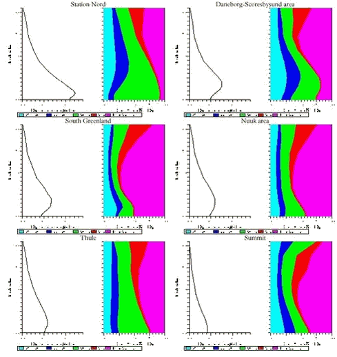
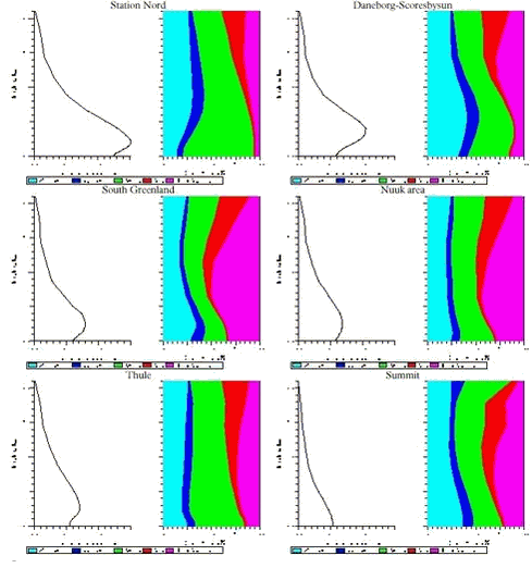
In Figures 1.3.6 and 1.3.7 the vertical distributions of SO_X and Pb and the contribution from different anthropogenic sources to these vertical distributions for 6 different areas at Greenland are shown. The areas are: Station Nord, Daneborg-Scoresbysund area, South Greenland, Nuuk area, Thule and Summit. As mentioned earlier the highest concentrations of both sulphur and lead are in the northern part of Greenland and it is in lowest 2 km of the atmosphere, while the lowest concentrations are at the icecap of Greenland (Summit). The highest concentration levels are a factor of 10 lower than the similarly calculated concentrations for Denmark.

View the image in full size
Figure 1.3.6.
The vertical distribution of SOX and contributions from different sources to the vertical contributions for Station Nord (upper left), Daneborg-Scoresbysund area (upper right), South Greenland (middle left), Nuuk area (middle right), Thule (lower left) and Summit (lower right)

The largest contribution to the atmospheric burden of sulphur and Pb is coming from the Russian sources with a contribution up to more than 50% in the northern part of Greenland, while in the southern and western part the most important sources are from North America (up to 50% for sulphur and 35 % for lead). At higher levels for whole Greenland there are larger contributions from the sources in North America.

View the image in full size
Figure 1.3.7.
The vertical distribution of Pb and contributions from different sources to the vertical contributions for Station Nord (upper left), Daneborg-Scoresbysund area (upper right), South Greenland (middle left), Nuuk area (middle right), Thule (lower left) and Summit (lower right)

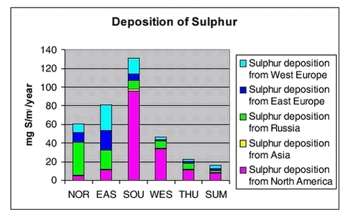
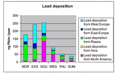
In Figures 1.3.8 and 1.3.9 the total deposition and the contribution from different sources are shown for the same 6 areas as shown above. The largest deposition of both sulphur and lead is in the southern part of Greenland and the lowest is at the icecap. The deposition levels for sulphur are a also factor 10 lower than the calculated deposition levels in Denmark, and for lead the deposition is a factor of 15 lower. The largest contribution to the deposition in Northern part of Greenland is coming from Russian sources (up to 60%), while for the Eastern part there are larger contributions from European sources (65%). In the southern and western part the most important source for the deposition is from North America (up to 73% for sulphur and 55% for lead)


Figure 1.3.8.
The contribution from different sources to the total deposition of sulphur for Station Nord (NOR), Daneborg-Scoresbysund area (EAS), South Greenland (SOU), Nuuk area (WES), Thule (THU) and Summit (SUM)

Figure 1.3.9
The contribution from different sources to the total deposition of Pb for Station Nord (NOR), Daneborg-Scoresbysund area (EAS), South Greenland (SOU), Nuuk area (WES), Thule (THU) and Summit (SUM)

1.3.3 Modelling of mercury 

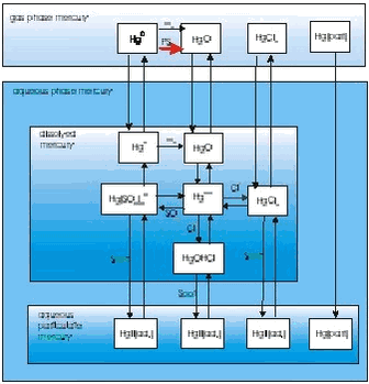
In general, activities aimed at modeling Hg are less developed, although major improvements in regional (European) and global modeling of Hg have been made. An example of a mercury model is the mercury version of the Danish Hemispheric Eulerian Model system (DEHM), which have been used to study the transport of mercury into the Arctic. The main reason for the development of the model was fulfill the recommendation from the AMAP workshop: “Modelling and sources: A workshop on Techniques and associated uncertainties in quantifying the origin and long-range transport of contaminants to the Arctic. Bergen, 14-16 June 1999” to “Assess spring Hg and O3 depletion using atmospheric model with high-resolution boundary layer”.

In the present mercury version of DEHM there are 13 mercury species, 3 in gas-phase (Hg⁰, HgO and H_gCl₂), 9 species in the aqueous-phase and 1 in particulate phase.
In the current version the emissions of anthropogenic mercury are based on the new global inventory of mercury emissions for 1995 on a 1^ox1^o grid (Pacyna & Pacyna, 2002), which includes emissions of Hg⁰, reactive gaseous mercury (RGM) and particulate mercury. There are no re-emissions from land and oceans, instead a background concentration on 1.5 ng/m³ of Hg⁰ is used as initial concentrations and boundary conditions.

The chemistry is based on the scheme from the GKSS model, see Figure 1.3.10 and Petersen et al. (1998). The mercury chemistry is depending on the concentrations of O₃, SO₂, Cl^- and Soot. Constant values of Cl^- and Soot concentrations are used, while O₃ and SO₂ concentrations are both obtained from the photochemical version of DEHM. During the polar sunrise in the Arctic an additional fast oxidation rate of Hg⁰ to HgO is assumed: Inside the boundary layer over sea ice during sunny conditions it is assumed that there is an additional oxidation rate of ¼ hour^-1. The fast oxidation stops, when surface temperature exceeds -4^oC. The removals of Hg0 are due to the chemistry and the uptake by cloud water.

Figure 1.3.10.
The GKSS chemical scheme used in the mercury model (from Petersen et al., 1998). The red arrow shows the additional fast oxidation rate of Hg⁰ to HgO during Polar Sunrise (PS).

The dry deposition velocities of the reactive gaseous mercury species are based on the resistance method, where the surface resistance similar to HNO₃ is used. The wet deposition of reactive and particulate mercury is parameterized by using a simple scavenging coefficients formulation with different in-cloud and below-cloud scavenging coefficients (see Christensen, 1997).

The mercury model has been run for October 1998 to December 2000. For the Arctic areas the model has been compared with measurements from Station Nord in northeast Greenland. The results show that there is some agreement between the calculated and observed concentrations of elemental mercury (Hg⁰), see Figure 1.3.11. The calculated concentrations of reactive gaseous mercury (RGM) and particulate mercury are also shown, and during the depletion period the levels of both species increase considerably.
Because the dry deposition velocity of RGM is very high, these high concentrations of RGM result to a dramatically increased deposition of mercury, which are shown in both Figures 1.3.12 and 1.3.13.

View the image in full size
Figure 1.3.11.
Comparisons between observed (blue curve) and calculated daily mean of Hg⁰ with two model versions, one without depletion (red) and one with depletion (black) (top) , the total particulate mercury (middle) and total reactive gaseous mercury (bottom) for Station Nord in North-Eastern Greenland.

View the image in full size
Figure 1.3.12.
The total deposition of mercury without Arctic mercury depletion (left) and with (right) in µg Hg/m²/month.

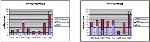
In Figure 1.3.12, the total deposition of mercury for the 1999 and 2000 is shown. This example shows the importance of the mercury depletion in the Arctic for the total deposition of mercury. The total deposition increases in the whole Arctic and the surrounding areas, and for the area north of the Polar Circle the total deposition of mercury increases from 89 to 208 tonnes pr. year due to the depletion according to the model runs.

In Figure 1.3.13 the total deposition of mercury in µg Hg/m²/year for 8 different localities (6 in Greenland, Faeroe Island and Denmark) are shown. The total deposition is splitted up in three components: the contribution from the deposition of RGM, chemical made particulate mercury and directly emitted particulate mercury. At the figure it is shown very clearly how important the depletion phenomena is for the deposition of mercury for the northern, western and Eastern Greenland. F.ex for the Thule area the total deposition of mercury is increased with a factor 3, while for the southern part for Greenland the depletion phenomena have only a minor influence on the mercury deposition. For all places closed to the ocean the total deposition is at the same levels at the southern part of Greenland and slightly lower than the depositions in Denmark. It is also shown that it is the increased deposition of RGM, which contributes mainly to the higher deposition rates. The contribution from directly emitted particulate mercury is very small in Greenland. It is mainly the large atmospheric reservoir of elemental mercury, which contributes to the deposition, and which all global emissions both anthropogenic and natural contributes to.

View the image in full size
Figure 1.3.13.
Total deposition of Mercury in µg Hg/m²/year splitted up in deposition of Reactive Gaseous Mercury, chemical made particulate mercury and directly emitted particulate mercury for two different model runs: without depletion (left) and with depletion (right), and for 8 different localities: Station Nord (NOR), Daneborg-Scoresbysund area (EAS), South Greenland (SOU), Nuuk area (WES), Thule (THU), Summit (SUM), Faeroe Island (FAE) and Denmark (DEN)

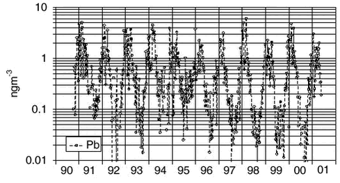
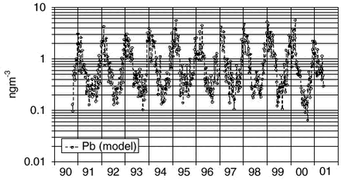
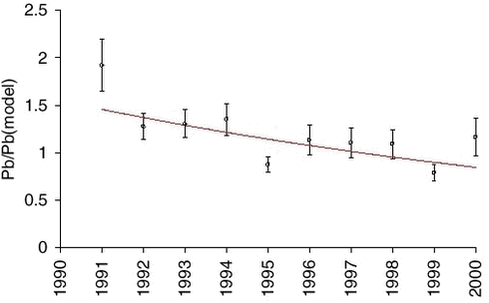
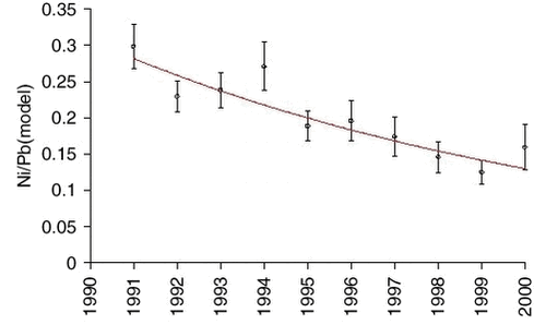
1.4 Trend analysis

1.4.1 Method and results

The chemical compounds and elements measured by IC and PIXE analysis in TSP samples and impregnated filter samples collected at Station Nord have been apportioned to four main source categories (Aarkrog er al. 1997). These are a ’soil’ source, (wind blown dust), a ’sea’ source (sea spray), a ’combustion’ source (a general anthropogenic source due to a variety of distant activities), and a ’metal’ source (probably due to copper-nickel production in the Arctic area). This is illustrated in Figure 1.2.4. Some elements have both an anthropogenic and a natural origin (e.g. vanadium, manganese and iron) while others are almost exclusively of anthropogenic origin: sulphur (except for a small amount of sea-salt sulphate), copper, nickel, zinc, arsenic and lead. These elements show a strong seasonal variation with high values in the winter/spring and very low values in the summer. Total sulphur (the sum of sulphur measured as sulphur dioxide and sulphate measured in the TSP samples) shows the same seasonal variation as the other anthropogenic elements. But the partition of the two components changes during the winter/spring season from a high content of sulphur dioxide during the dark winter period to a very low content after the polar sunrise in early spring.

Station Nord is almost not influenced by local or regional air pollution and can be considered as a remote watchtower from where the average emissions in a huge emission area in the eastern part of Europe and Russia can be followed. A study of the general emission trends is therefore possible using the long-time series of measurements during the last decade of the anthropogenic elements: Sulphur, copper, nickel, zinc, arsenic and lead. But, unfortunately, the measured concentrations depend strongly upon the meteorological conditions along the pathway to the Arctic. In the summer time the emissions never get to the Arctic, and during the winter the transport time can change much from week to week. Therefore, the single samples reflect only poorly the actual emissions in the source areas, and a trend analysis on the raw concentration data might give misleading results.
Fortunately, a relevant way to handle this problem was possible using the results of the hemispheric Eulerian model DEHM.

The DEHM model was run with emission data for the year 1989 for lead and with emission data for the year 1990 for sulphur for the 11-year period 1991-2001, where the emissions were kept constant through all the years. All the variations of the modelled concentrations at Station Nord are therefore due to changes in the meteorological conditions from day to day. The raw concentration data for lead (Pb) are shown in a logarithmic presentation in Figure 1.4.1, and the model calculations are shown in an analogous way in Figure 1.4.2. It is evident that the model to a high extent grasps the meteorological variations, although it underestimates the annual relative span. It might also be suggested from a comparison of the two figures that the measured data have a decreasing trend. The trend is much more clear in Figure 1.4.3 where the ratio Pb(measured)/Pb(model) has been calculated by weighted regression analysis for each of the years 1991-2000 (Wåhlin et al., 2002). The values are fitted by an exponential function of time. It can be seen that this trial function does not disagree statistically with the data points when the uncertainties (standard deviations) are taken into account. Thus, assuming an exponential decay of the emissions, the half-value period and its standard deviation could be estimated at 11 ± 3 years.

Figure 1.4.1.
Concentrations of particulate lead (Pb) measured at Station Nord in the years 1990-2001.

 
Figure 1.4.2.
Concentrations of airborne particulate lead (Pb) at Station Nord calculated using the Hemispheric Eulerian model with constant emission data (for the year 1989).

Figure 1.4.3.
Ratios determined by regression analysis of measured values and constant emission model values of lead (Pb) for each of the years 1991-2000. The values are fitted by an exponential function of time with a half-value period of 11 ± 3 year

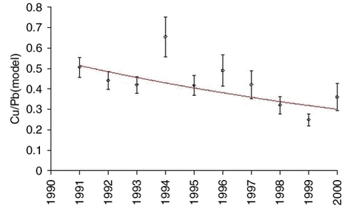
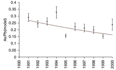
The measurements of arsenic (As) and zinc (Zn) are highly correlated with lead on a sample to sample basis, and also the measurements of nickel (Ni) and copper (Cu) on a seasonal basis. Therefore, it makes sense to use the model values of lead for an equivalent analysis of trends for the other elements. The influence of the large scale meteorological conditions seems to be very similar. Ratios and exponential trend functions were determined by the same technique used for lead. The results are presented in Table 1.4.1 and Figures 1.4.4-1.4.7. The constant exponential trend seems to give a good description for all elements.


Table 1.4.1.
Ratios (measured mass/model mass) determined by regression analysis, and half-value periods of fitted exponential functions.  

Figure 1.4.4.
Ratios determined by regression analysis of measured values of copper (Cu) and constant emission model values of lead (Pb) for each of the years 1991-2000. The values are fitted by an exponential function of time with a half-value period of 12±3 year^.

 
Figure 1.4.5.
Ratios determined by regression analysis of measured values of zinc (Zn) and constant emission model values of lead (Pb) for each of the years 1991-2000. The values are fitted by an exponential function of time with a half-value period of 12±3 year.

Figure 1.4.6.
Ratios determined by regression analysis of measured values of nickel (Ni) and constant emission model values of lead (Pb) for each of the years 1991-2000. The values are fitted by an exponential function of time with a half-value period of 8.1±1.3 year.

Figure 1.4.7.
Ratios determined by regression analysis of measured values of arsenic (As) and constant emission model values of lead (Pb) for each of the years 1991-2000. The values are fitted by an exponential function of time with a half-value period of 12±3 year.

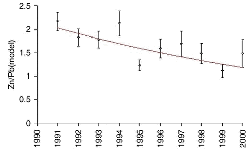
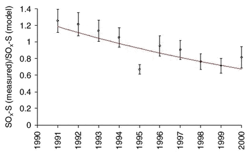
The anthropogenic sulphur is emitted to the atmosphere as sulphur dioxide and is converted to sulphuric acid (sulphate) by photochemical processes. The Hemispherical Eulerian Model (DEHM) takes this conversion into account, and also the different deposition rates of sulphur dioxide (gas) and sulphate (particles) are included in the model. The DEHM model was run with constant sulphur emission data for the year 1990 for the 11-year period 1991-2001. The results for Station Nord were expressed as total-sulphur SO_x-S (sum of the elemental sulphur mass in sulphur dioxide and sulphuric acid/sulphate, SO₂-S+SO₄-S) and compared with thecorresponding measured values of SO_x-S. No correction for sea salt sulphate was made as the average amount at Station Nord is relatively small (approx. 7%). Following exactly the same procedure as for lead, the ratio SO_x-S(measured)/SO_x-S(model) was calculated by regression analysis for each of the years 1991-2000. The results are shown in Figure 1.4.8 and Table 1.4.2. It can be seen the declining trend is similar to the trend of the other anthropogenic elements.

Figure 1.4.8.
Ratios determined by regression analysis of measured values of sulphur (SO_x-S) and constant emission model values for each of the years 1991- 2000. The values are fitted by an exponential function of time with a half-value period of 11 ± 2 year.

Table 1.4.2.
Ratios (measured mass/model mass) determined by regression analysis, and half-value period of a fitted exponential function.  

1.5 Conclusions

The High Arctic is burdened with a considerable atmospheric pollution, consisting of a wide variety of acidic and toxic compounds, which originate in mid-latitude industrial areas. That has been demonstrated by the combined use of long-term field measurements and sophisticated large-scale meteorological and chemical transport models. The pollution reaches it’s maximum in late winter and early spring when atmospheric circulation favours transport from these source areas into the Arctic region. This Arctic Haze is accompanied by an intense photochemical activity inducedin the Arctic atmosphere by the Polar sunrise. Much of this pollution leaves the Arctic region again but a considerable amount is deposited on land and sea surfaces, leading to detrimental effects on the vulnerable eco-systems in this pristine region.

Particular interest has been attached to mercury as an atmospheric pollutant. It has been found that this volatile heavy metal has a unique behaviour in the Arctic spring atmosphere. After Polar sunrise in February gaseous elemental mercury (GEM) is abruptly depleted from the atmosphere in the so called mercury depletion episodes lasting from hours to days whereupon it is equally abruptly restored to the original concentrations of about 1.5 ng·m^-3. MDE has been found at several Arctic stations and MDE therefore seems to be a ubiquitous phenomenon in Arctic. The MDE leads to deposition of atmospheric mercury at a time where the Arctic biological system is extremely active and thus the deposited mercury may be bioaccumulated much more effectively than predicted from mid-latitudes studies.

MDE occurs simultaneously with the depletion of ozone. Halogen radicals as Cl, ClO, Br and BrO have been suggested to be responsible for MDE. In the present report strong evidence is found for that Br is the only important reactant.

The model calculations have shown that different source regions have a different influence in various parts of Greenland because of differing pathways. Thus the atmospheric concentrations of sulphur in the central, southern and south-western areas of Greenland are dominated by source regions (in order of decreasing dominance) in North America, Russia and Western Europe. The concentrations in the northern and eastern Greenland are dominated by sources in Russia, North America and Europe as a whole. For lead the influences are much the same, but with a tendency for higher relative contributions from Western Europe. The average concentrations are by far the largest in northeast Greenland.

For deposition of sulphur and lead it has been found that Russian sources dominate in the North and East over contributions from European sources. In the West and the South the contributions to the deposition come primarily from North America and secondarily from Europe. The depositions are largest in the South and East with north-eastern Greenland a close third.

The combination of field data and model calculations has also been highly useful in assessing trends in atmospheric concentrations. A glance at the concentrations during the 1990s shown in Figures 1.4.1 and 1.4.2 may, depending on the reader’s subjective assessments, either lead to a conviction that there is a downward trend in these data or that there is no trend because of a large spread in data. This large spread is mainly caused by the varying meteorological conditions in the different years. Most likely a simple statistical analysis would show that there is a downward trend but that it is not significant.
A much smaller scatter is found when experimental data and are compared to model data, calculated under the assumption that emissions have remained unchanged during the decennium. The ratios between measured and model values were found for each of the years 1991-2000 using regression analysis. An assessment of these timeseries have shown that there indeed are significant decreases in the concentrations, contrary to the built-in assumption that emissions have been unchanged. Since the DEHM model estimates that more than 70% of the sulphur and lead measured at Station Nord is emitted in the area covering the former Soviet Union the results of the trend analysis indicate that the general anthropogenic atmospheric emissions decreased significantly in this region in the nineties. Whether the internationally agreed emission reductions that have mainly been effected in Western Europe and North America also influence the results from Station Nord is, however, not clear. Thus the effect on ambient concentrations of the stronger decline of the lead emissions compared with the decline of the sulphur emissions, which has been observed in Western Europe, is not observed at Station Nord.

It can however be stated that the smaller emissions in the source areas have taken effect also in the High Arctic and that the decreasing trends for Pb, Zn, Ni, As, Cu and S can be characterised by a half-life of about 11 years.

1.6 References

Aarkrog, A., P. Aastrup, G. Asmund, P. Bjerregaard, D. Boertmann, L. Carlsen, J. Christensen, M. Cleemann, R. Dietz, A. Fromberg, E. Storr-Hansen, N. Z. Heidam, P. Johansen, H. Larsen, G. B. Paulsen, H. Petersen, K. Pilegaard, M.E. Poulsen, G. Pritzl, F. Riget, H. Skov, H. Spliid, P. Weihe & P. Wåhlin: AMAP Greenland 1994-1996. Arctic Monitoring and Assessment Programme (AMAP). Under the series “Enviromental Project from the Danish Environmental Protection Agency". Report Nr. 356, 1997, 792 pp.

Ariya,P.A Khalizov & A. Gildas, 2002. Reactions of Gaseous Mercury with Atomic and Molecular Halogens: Kinetics, Product Studies, and Atmosphere Implications. J. Phys. Chem. in Press.

Barrie, L. A., Y. Yi, U. Lohmann, W.R.Leaitch, P. Kasibhatla, G.-J. Roelofs, J. Wilson5, F. McGovern, C. Benkovitz, M.A. Meliere, K. Law, J. Prospero, M. Kritz, D.Bergmann, C. Bridgeman, M. Chin, J. Christensen, R. Easter, J. Feichter, A. Jeuken, E. Kjellstrom, D. Koch, C. Land, P. Rasch, 2001. A comparison of large scale atmospheric sulphate aerosol models (cosam): overview and highlights. Tellus, 53B, pp 615-645

Benkowitz, C. M., T. Scholtz, J. Pacyna, L. Tarrasón, J. Dignon, E. Voldner, P. A. Spiro & T. E. Graedel, 1996. Global Gridded Inventories of Anthropogenic Emissions of Sulphur and Nitrogen. J. Geophys. Res., 101: 29239-29253.

Boudries, H. & J.W. Bottenheim, 2000. Cl and Br Atom Concentrations During a Surface BoundaryLayer Ozone Depletion Event in the Canadian High Arctic. Geophys. Res. Lett. 27 (4): 517-520.

Christensen, J., 1995. Transport of Air Pollution in the Troposphere to the Arctic. PhD thesis. National Environmental Research Institute, DK-4000 Roskilde, Denmark, 377 pp.

Christensen, J., 1997. The Danish Eulerian Hemispheric Model - A Three Dimensional Air Pollution Model Used for the Arctic. Atm. Env, 31: 4169-4191.

Christensen, J., 1999. An overview of Modelling the Arctic mass budget of metals and sulphur: Emphasis on source apportionment of atmospheric burden and deposition. In: Modelling and sources: A workshop on Techniques and associated uncertainties in quantifying the origin and long-range transport of contaminants to the Arctic. Report and extended abstracts of the workshop, Bergen, 14-16 June 1999. AMAP report 99:4. see also http://www.amap.no/

Christensen J.H., N.Z. Heidam, H. Skov & P. Wåhlin, 2000. AMAP Atmospheric monitoring and modelling in Greenland 1998-1999, NERI.

Christensen J.H., N.Z. Heidam, H. Skov & P. Wåhlin, 2001. AMAP Atmospheric monitoring and modelling in Greenland 2000, NERI.

Dastoor A. P., & J. Pudykiewicz, 1996.. A Numerical Global Meteorological Sulphur Transport Model and its Application to Arctic Air Pollution. Atmospheric Environment, 30: 1501-1522.

DeMore, Sander, S.P. Golden, D.M. Hampson, R.F. Kurylo, M.J. Howard, C.J. Ravinshankara, A.R. Kolb & M.J.Milina, 1997. Chemical Kinetics and Photochemical Data for Use in Stratospheric Modeling. Evaluation No. 12. JPL Publication 97-4. NASA.

Ebinghaus, R. H. Kock, C Temme, J.W. Einax, A.G. Löwe, A. Richter, J.P Burrows, W.H. Schroeder, 2002. Antarctic Springtime Depletion of Atmospheric Mercury. E. S. T. 36: 1238-1244.

Goodsite, M.E., S.B. Brooks, S.E.Lindberg, T.P. Meyers, H Skov, M.R.B. Larsen, & C. Laurent, 2002. Measuring reactive gaseous mercury flux by relaxed eddy accumulation using KCl coated annular denuders. Under preparation.

Grandjean, P., P. Weihe, R.F. White, & F. Debes, 1998. Cognitive Performance of Children Prenatally Exposed to “Safe” Levels of Methyl Mercury. Env. Res. 77A: 165-172.

Grell, G. A., J. Dudhia & D.R. Stauffer D. R., 1995: A Description of the Fifth-Generation Penn State/NCAR Mesoscale Model (MM5). NCAR/TN-398+STR. NCAR Technical Note. June 1995, pp. 122. Mesoscale and Microscale Meteorology Division. National Center for Atmospheric Research. Boulder, Colorado.

Hausmann, M. & U. Platt, 1994. Spectroscopy measurement of bromine oxide and ozone in the high Arctic during Polar Sunrise Experiment 1992. J. Geophys Res. 99 (D12), 25: 399-25,413.

Iversen, T. 1989. Numerical Modelling of the Long Range Atmospheric Transport of Sulphur Dioxide and Particulate Sulphate to the Arctic. Atmospheric Environment, 23: 2571-2595.

Jobson, B.T., H. Niki, Y. Yokouchi, J. Bottenheim, F. Hopper, & R. Leaith, 1994. Measuremnts of C₂-C₆ hydrocarbons during the Polar Sunrise 1992 Experiment: Evidence for Cl atom and Br atom chemistry. J. Geophys. Res. 99 (D12), 25: 355-25,368.

Kämäri, J., P. Joki—Heiskala, J. Christensen, E. Degerman, J. Derome, R. Hoff & A.-M Kähkönen: Acidifying Pollutants, Arctic Haze, and Acidifications in the Arctic, Chapter 9 in: AMAP Assesment Report: Arctic Pollution Issues. Arctic Monitoring and Assessment Programme (AMAP). S. Wilson, J. Murray and H. Huntington, Ed, 1998.

Lin, C.-J. & S.O. Pehkonen, 1999. The Chemistry of tropospheric mercury: a review. Atm. Env. 33: 2067-2079

Lindberg, S. S. Brooks, S.-J. Lin, K. Scott, M.S. Landis, R.K. Stenens, M. Goodsite & A. Richter, 2002. Dynamic Oxidation of gaseous Mercury in the Arctic Troposphere at Polar Sunrise. E. S. T. 36 (6): 1245-1256.

Lohmann, U., W.R. Leaitch, K. Law, L. Barrie, Y. Yi, D. Bergman, C, Bridgeman, M. Chin, J. Christensen, R. Easter, J. Feichter, A. Jeuken, E. Kjellstrom, D. Koch, C. Land, P. Rasch, G.-J Roelof:, 2001 Vertical distributions of sulphurspecies simulated by large scale atmospheric models in cosam: Comparison with observations. Tellus, 53B, pp 646-672

Pacyna, E.G., & J.M. Pacyna, 2002. Global emission of mercury from anthropogenic sources in 1995. Water, Air, and Soil Pollution 137: 143-165.

Pacyna, J. M., M. Trevor Scholtz & Y-F. Li, 1995. Global Budgets of Trace Metal Sources, Environmental Reviews, 3: 145-159.

Petersen, G., J. Munthe, K. Pleijel, R. Bloxam, & A. Vinod Kumar, 1998. A comprehensive eulerian modeling framework for airborne mercury species: development and testing of the tropospheric chemistry module (TCM). Atm.Env. 32: 829-843.

Platt U. & G.K. Moortgat, 1999. Heterogeneous and Homogeneous Chemistry of reactive Halogen Compounds in the Lower Troposphere. J. Atm. Chem. 34: 1-8.

Roelofs, G.J., P. Kasibhatla, L. Barrie, D. Bergmann, C, Bridgeman, M. Chin, J. Christensen, R. Easter, J. Feichter, A. Jeuken, E. Kjellström, D. Koch, C. Land, U. Lohmann, P. Rasch, 2001. Analysis of regional budgets of sulfur species modelled for the COSAM exercise. Tellus, 53B, pp 673-694

Röckmann, T., A.M. Brenninkmeijer, P.J. Crutzen & U. Platt, 1999. Short –term variations in the ¹³C/¹²C ratio of CO as a measure of Cl activation during tropospheric ozone depletion events in the Arctic. J. Geophys. Res. 104 (D1): 1691-1697.

Schroeder, W.H., K.G. Anlauf,L.Y. Barrie, A Lu, D.R. Schneebeerger & T. Berg, 1998. Arctic springtime depletion of Mercury. Nature, 394: 331-332.

Skov, H., M.E. Goodsite, J. Christensen, G.Geernaert, N.Z. Heidam, & B. Jensen,. "Atmospheric Mercury and ozone at Station Nord, Northeast Greenland,” Under preparation 2002

Sommar, J., 2001. The Atmospheric Chemistry of Mercury. Ph.D. Dissertation. Chalmers Reproservice, Gothenburg, Sweden

Tarrasón, L. & T. Iversen, 1992. The Influence of North American Anthropogenic Sulphur Emissions over Western Europe. Tellus, 44B:, 114-132.

Tarrasón, L., J. Bartnicki & T. Iversen, 1997. Sources, Transport and Atmospheric Distribution of Sulphur and Lead in the Arctic. In “ The AMAP International Symposium on Environmental Pollution in the Arctic. Extended abstracts. Tromsø, Norway June 1-5, 1997”. 239-241.

Tuckermann, M., R. Ackermann, C. Gölz, H. Lorenzen-Schmidt, T. Senne, J. Stutz, B. Trost, W. Unold & U. Platt, 1997. DOAS-observation of halogen radical-catalysed arctic boundary layer ozone destruction during ARCTOC-campaigns1995 and 1996 in Ny-Ålesund, Spitsbergen. Tellus. 49B: 533-555.

Wåhlin P., 1993. A multivariate receptor model with a physical approach. Proceedings of the Fifth International Symposium on Arctic Air Chemistry, September 8-10, 1992, Copenhagen.

Wåhlin, P., J. Christensen & N.Z. Heidam, 2002. Emission trends of anthropogenic elements observed from a remote site in North-eastern Greenland, 1990-2001. In preparation.

| Front page | | Contents | | Previous | | Next | | Top |