Pesticides Research no. 63, 2004
Scenarios and Model Describing Fate and Transport of Pesticides in Surface Water for Danish Conditions
Contents
1 Choice of Scenario Description
- 1.1 Process considerations
- 1.1.1 Spray drift
- 1.1.2 Wet and Dry Deposition
- 1.1.3 Deposition onto the Soil Surface and Plants
- 1.1.4 Dissolved in Surface Runoff or Transported with Soil Erosion
- 1.1.5 Unsaturated zone
- 1.1.6 Groundwater
- 1.1.7 Pesticide dissolved in drain flow
- 1.1.8 Colloid-bound Pesticide in Drain Flow
- 1.1.9 Overview of Pathways
- 1.1.10 Measurements in Streams
- 1.1.11 Measurements in Ponds
- 1.2 Considerations of Scale
2 Selection of "Representative" Areas
- 2.1 Soil types and hydrology
- 2.2 Overall Land Use
- 2.3 Hydrology of water bodies
- 2.4 Climate
- 2.5 Changes discovered during project implementation
3 Changes from Calibrated Catchments to Scenarios
- 3.1 Lillebæk stream
- 3.2 Odder bæk
- 3.3 The pond scenarios
- 3.3.1 Geomorphology
- 3.3.2 Pond Type around Odder Bæk
- 3.3.3 Pond Type around Lillebæk
- 3.3.4 Conclusions regarding types of ponds
- 3.3.5 Dimensions of the Ponds
- 3.3.6 Biological structure of the pond
- 3.3.7 Implementation of the pond in the Lillebæk model setup
- 3.3.8 Implementation of the pond in the Odder Bæk model setup
4 Parameterisation of Sub-components
- 4.1 Growth curves and deposition on soils
- 4.2 Wind drift
- 4.3 Dry deposition
- 4.4 Calculation of effective pesticide dose on the soil
- 4.5 Adsorption to macrophytes
- 4.6 Adsorption to suspended matter
- 4.7 Sediment in streams and ponds
5 General Conditions for the Simulations
7 Uncertainty Issues in Relation to the Scenarios
- 7.1 Introduction
- 7.2 Uncertainties related to model choice and model parameterisation
- 7.3 Uncertainties related to the choice of scenarios
- 7.4 Uncertainties related to input
- 7.5 Uncertainties related to the interpretation of output
- 7.6 Strategies to further reduce the uncertainty
8 Uncertainty Analysis of the Registration Model
- 8.1 General systematic in uncertainty analysis
- 8.2 Principle of the uncertainty analysis - intelligent Monte Carlo
- 8.3 Uncertainty on the quantification of the variance
- 8.4 Implementation in to the user interface
Appendix A: Description of Soil Types in the Test Catchments at the Time of Selection
Appendix D: Uncertainty Analysis of the Registration Model
Appendix E: Monthly water balances for the scenarios
Preface
The project ”Model Based Tool for Evaluation of Exposure and Effects of Pesticides in Surface Water”, funded by the Danish Environmental Protection Agency, was initiated in 1998. The aim of the project was:
To develop a model-based tool for evaluation of risk related to pesticide exposure in surface water. The tool must be directly applicable by the Danish Environmental Protection Agency (DEPA) in their approval procedure. As part of this goal, the project had to:
- Develop guidelines for evaluation of mesocosm experiments based on a system-level perspective of the fresh water environment.
- To develop models for deposition of pesticides on vegetation and soil.
- To estimate the deposition of pesticides from the air to the aquatic environment.
The project, called ”Pesticides in Surface Water”, consisted of seven subprojects with individual objectives. The sub-projects are listed in Table 1.
Table I Sub-projects of ”Pesticides in Surface Water”.
Tabel I Oversigt over delprojekter i ”Pesticider i overfladevand”.
| Title | Participating institutions | |
| A | Development and validation of a model for evaluation of pesticide exposure | DHI Water & Environment |
| B | Investigation of the importance of plant cover for the deposition of pesticides on soil | Danish Institute of Agricultural Science |
| C | Estimation of addition of pesticides to surface water via air | National Environmental Research Institute Danish Institute of Agricultural Science |
| D | Facilitated transport | DHI Water & Environment |
| E | Development of an operational and validated model for pesticide transport and fate in surface water | DHI Water & Environment National Environmental Research Institute |
| F | Mesocosm | DHI Water & Environment National Environmental Research Institute |
| G | Importance of different transport routes in relation to occurrence and effects of pesticides in streams | National Environmental Research Institute County of Funen County of Northern Jutland |
Figure I Links between the different sub-projects. The sub-projects are placed on a cross-section of the catchment to illustrate interactions.
Figur I Sammenhæng mellem delprojekterne. Delprojekterne er placeret på et tværsnit af en opland for at illustrere interaktionerne.
Figure 1 describes the relationship between the sub-projects. Sub-project 1 models the upland part of the catchment, while sub-project 5 models surface water bodies. Sub-project 8 delivers data to both modelling projects. Sub-project 2 and 3 develops process descriptions for wind drift, dry deposition and deposition on soils. Sub-project 4 builds and tests a module for calculation of colloid transport of pesticide in soil. The module is an integrated part of the upland model. Sub-project 6 has mainly concentrated on interpretation of mesocosm-studies. However, it contains elements of possible links between exposure and biological effects.
The reports produced by the project are:
- Styczen, M., Petersen, S., Christensen, M., Jessen, O.Z., Rasmussen, D., Andersen, M.B. and Sørensen, P.B. (2004a): Calibration of models describing pesticide fate and transport in Lillebæk and Odder Bæk Catchment. - Ministry of Environment, Danish Environmental Protection Agency, Pesticides Research No. 62.
- Styczen, M., Petersen, S. Sørensen, P.B., Thomsen, M and Patrik, F. (2004b): Scenarios and model describing fate and transport of pesticides in surface water for Danish conditions. - Ministry of Environment, Danish Environmental Protection Agency, Pesticides Research No. 63.
- Styczen, M., Petersen, S., Olsen, N.K. and Andersen, M.B. (2004c): Technical documentation of PestSurf, a model describing fate and transport of pesticides in surface water for Danish Conditions. - Ministry of Environment, Danish Environmental Protection Agency, Pesticides Research No. 64.
- Jensen, P.K. and Spliid, N.H. (2003): Deposition of pesticides on the soil surface. - Ministry of Environment, Danish Environmental Protection Agency, Pesticides Research No. 65.
- Asman, W.A.H., Jørgensen, A. and Jensen, P.K. (2003): Dry deposition and spray drift of pesticides to nearby water bodies. - Ministry of Environment, Danish Environmental Protection Agency, Pesticides Research No. 66.
- Holm, J., Petersen, C., Koch, C. and Villholth, K.G. (2003): Facilitated transport of pesticides. - Ministry of Environment, Danish Environmental Protection Agency, Pesticides Research No. 67.
- Helweg, C., Mogensen, B.B., Sørensen, P.B., Madsen, T., Rasmussen, D. and Petersen, S. (2003): Fate of pesticides in surface waters, Laboratory and Field Experiments. Ministry of Environment, Danish Environmental Protection Agency, Pesticides Research No. 68.
- Møhlenberg, F., Petersen, S., Gustavson, K., Lauridsen, T. and Friberg, N. (2001): Guidelines for evaluating mesocosm experiments in connection with the approval procedure. - Ministry of Environment and Energy, Danish Environmental Protection Agency, Pesticides Research No. 56.
- Iversen, H.L., Kronvang, B., Vejrup, K., Mogensen, B.B., Hansen, A.M. and Hansen, L.B. (2003): Pesticides in streams and subsurface drainage water within two arable catchments in Denmark: Pesticide application, concentration, transport and fate. - Ministry of Environment, Danish Environmental Protection Agency, Pesticides Research No. 69.
The original thoughts behind the project are described in detail in the report ”Model Based Tool for Evaluation of Exposure and Effects of Pesticides in Surface Water”, Inception Report – J. nr. M 7041-0120, by DHI, VKI, NERI, DIAS and County of Funen, December, 1998.
The project was overseen by a steering committee. The members have made valuable contributions to the project. The committee consisted of:
- Inge Vibeke Hansen, Danish Environmental Protection Agency, chairman 1998-mid 2000.
- Jørn Kirkegaard, Danish Environmental Protection Agency (chairman mid-2000-2002).
- Christian Deibjerg Hansen, Danish Environmental Protection Agency
- Heidi Christiansen Barlebo, The Geological Survey of Denmark and Greenland.
- Mogens Erlandsen, University of Aarhus.
- Karl Henrik Vestergaard, Syngenta Crop Protection A/S.
- Valery Forbes, Roskilde University.
- Lars Stenvang Hansen, Danish Agricultural Advisory Centre (1998-2001).
- Poul-Henning Petersen, Danish Agricultural Advisory Centre (2002).
- Bitten Bolet, County of Ringkøbing (1988-1999).
- Stig Eggert Pedersen, County of Funen (1999-2002).
- Hanne Bach, The National Environmental Research Institute (1999-2002).
October 2002
Merete Styczen, project co-ordinator
Sammenfatning og konklusioner
Når nye pesticider skal registreres til brug i Danmark, har Miljøstyrelsen behov for at kunne bedømme, om miljøet vil blive påvirket i uacceptabel grad. På baggrund af de indsendte data vurderes stoffets egnethed som pesticid under danske forhold. Bedømmelsen foregår i ”tiers” som er en slags screeningssystem. Først bedømmer man stoffet under temmelig urealistiske, men simple forhold (tier 1). Forventes stoffet ikke at skade organismer under disse forhold, kan det godkendes. Ellers forsøges igen under mere virkelighedsnære forhold (tier 2). Flere tiers kan bygges på for at sandsynliggøre, at et stof kan anvendes uden risici, eventuelt under visse specielle forhold.
Slutproduktet i projektet ”Pesticider i Overfladevand” er et modelværktøj (PestSurf), der kan anvendes i forbindelse med registrering af nye pesticider på tier 2-niveau eller højere. Pestsurf bygger på modeller over to eksisterende oplande. Det antages, at de to grundmodeller kan repræsentere nogle velkendte danske forhold. På en række udvalgte punkter modificeres modellerne for at fremstå mere egnede til en generel risiko-analyse.
For at sikre at alle relevante transport- og omsætningsprocesser blev representeret i modellen, indledtes arbejdet med en litteraturgennemgang. Forskellige arbejdsgrupper har derefter arbejdet med de dårligst belyste transport-og omsætningsbeskrivelser. Arbejdsgrupperne har specificeret, hvorledes deres delkomponent skulle medtages i de endelige scenarier. Det gælder vinddrift, tørdeposition, afsætning på jordoverfladen og kolloidtransport.
Der er så langt som muligt taget hensyn til retningslinier givet af EU's FOCUS-grupper, der arbejder med modeller til brug i pesticidregistrering.
Selv om scenarierne skal være virkelighedstro, er der undervejs i deres opbygning taget en række beslutninger vedrørende beskrivelser og parametervalg, der vil have betydning for risikovurderingen. Pojektets styregruppe været derfor været involveret i alle beslutninger vedrørende parametersætning, når der har været tvivl om valgene.
Der er opstillet et vandløbsscenarie for hvert af de to oplande, baseret på de kalibrerede modeller. I det lerede opland er den rørlagte del af vandløbet åbnet i scenariet for at sikre mest muligt vinddrift, men ellers er modellerne fysisk set ens. I scenarierne foregår vinddrift og tørdeposition altid vinkelret på vandløbet, og følger de gennemsnitlige vindforhold. I scenarierne er hele landbrugsarealet dækket af en afgrøde, der sprøjtes ad en gang. Dette er ikke umiddelbart realistisk for større oplande, men for nogle afgrøder eller pesticider er den faktiske dækningsgrad i små oplande høj. Eksisterende usprøjtede zoner langs vandløbene sprøjtes imidlertid ikke. Brugeren kan vælge at indsætte usprøjtede zoner af forskellig vidde, hvis vinddrift er en vigtig kilde.
Vandhullerne i scenarierne er kunstige, idet der ikke i projektet måltes på vandhuller i det to oplande. Der eksisterer altså ingen data at kalibrere imod. Men allerede i projektets startfase defineres nogle standard-vandhuller for danske forhold, som så er forsøgt indlagt i de to oplande. Den ene type vandhul (mest almindelig på sandjord) står i direkte forbindelse med grundvandet. Den anden type (på moræneler), er betinget af at infiltrationen til underliggende lag er langsom. Den første type er indlagt i det sandede opland, den anden i det lerede opland, og oplande er defineret, der fører til søer på 200-500 m2, der ikke tørrer ud og har en typisk niveau-variation på 1 m. For at kunne tage højde for betydningen af vandhullernes biologiske struktur og belastning med næringssalte kan der som en del af scenarierne vælges mellem makrofyt (vandplante)-dominerede vandhuller med lav belastning af næringssalte og fytoplankton-dominerede vandhuller med høj belastning med næringssalte.
Scenarierne er bygget ind i en brugerflade, der styrer overførslen af pesticiddata, valget af afgrøde, sprøjtetidspunkt og dosis samt bredden af den sprøjtefri zone til de tilgrundliggende modeller. Alle vandberegninger er udført på forhånd, og kan ikke ændres af brugerne. Desuden indeholder modellen oplysninger om en række parametre af betydning for skæbnen og transporten af pesticiderne som er fastlagt gennem kalibreringer.
De faste værdier følger, i det omfang det er muligt, de anbefalinger, som FOCUS-grupperne i EU har opstillet for denne type beregninger (FOCUS 2000, 2002). I EU-sammenhæng anvender man en række separate modeller til forskellige delkomponenter (overfladisk afstrømning, drænvand, grundvand og vandløb/åbent dræn/vandhul), opstillet på hypotetiske situationer. Resultatet er at den hydrologiske sammenhæng er dårligere, end hvad det er lykkedes at få frem her, samt at det samlede system ikke kan valideres.
Projektet er stødt på uforudsete problemer, hvoraf nogle kan håndteres gennem en usikkerhedsvurdering, og andre er mere generelle. For eksempel kræver de detaljerede beregninger meget beregningstid, og det blev vedtaget tidligt i projektet at udføre de nødvendige vandberegninger ”på forhånd” og gennemføre stofberegningerne ”ovenpå” for at spare tid. Imidlertid gør den ønskede fine tidsmæssige opløsning af vandberegnings-resultaterne dem så omfattende, at det har været nødvendigt at give køb på simuleringsperiodens længde. Simuleringsperiodens længde er nu 8 år men kun de sidste 4 år er udvalgt som basis for evalueringen af pesticiderne. De udvalgte år representerer så vidt muligt klimavariationerne i den sidste 10-års-periode.
De problemer, der er observeret i forbindelse med kalibreringerne for henholdsvis det lerede og det sandede opland vil også gælde for scenarierne. Det gælder problemer i forbindelse med makropore-parameterisering og til en vis grad evnen til at fange de meget skarpe pesticidtoppe i drænvand på grund af for stor opblanding af drænvandet med det øvrige grundvand. Generelt overvurderes koncentrationerne i det lerede opland og undervurderes i det sandede.
De anvendte forudsætninger vedrørende vinddrift og sprøjtet areal betyder, at koncentrationen i vandløbene bliver ret høj. Vinddriftstoppene, og i nogen tilfælde tørdeposition, er langt de største beregnede belastninger når bufferzonen er lille. Dette svarer til hvad FOCUS modellerne, der anvendes i EU-regi, finder, men ikke til hvad der blev fundet projektets måleprogram. Der er dog også en betydelig transport via dræn.
Modellen har en finere tidslig opløsning end man før har anvendt i risikovurdering, og beskriver vinddriftsbelastninger i vandløb og vandhuller. Men for drænafstrømning sætter filstørrelserne en grænse for hvor detaljeret opløsningen kan blive, og høje koncentrationer i korte afstrømningshændelser kan være vanskelige at beskrive.
Mens scenariet, bygget over det lerede opland, lever op til de oprindeligt stillede krav, har visse af forudsætningerne for valget af det sandede opland vist sig ikke at holde. Teksturen er lidt mere leret end forventet, og makroporer, som ellers ikke skulle findes her, synes at have en effekt på de simulerede koncentrationer. Man må derfor stille spørgsmål ved om det scenarie opfylder Miljøstyrelsens oprindelige forventninger.
For at øge modellens anvendelighed bør der gøres en yderligere indsats, for at få de identificerede problemer med procesbeskrivelser og tidslig opløsning ryddet af vejen.
Summary and conclusions
In connection with registration of new pesticides, the Danish Environmental Protection Agency (Danish EPA) needs to evaluate whether the environment will be affected to an unacceptable degree. Based on the submitted data, the appropriateness of the pesticide is evaluated for Danish conditions. The evaluation is carried out in ”tiers” which is a type of screening system. First, the compound is evaluated under rather unrealistic but simple conditions (tier 1). If the compound is unlikely to damage organisms under these conditions, it can be registered for use. Otherwise the evaluation is carried out again for more realistic conditions (tier 2). More tiers can be used, to substantiate that a compound can be used without risk, perhaps only under special conditions.
The end-product of the project ”Pesticides in Surface Water” is a model tool (PestSurf) that can be used in the registration procedure for new pesticides at tier 2-level or higher. PestSurf is based on models of two existing catchments. It is assumed that the two basic models represent certain well known Danish conditions. On selected points the basic models are modified to make them more appropriate as general risk analysis tools.
To ensure that all relevant transport- and transformation processes were represented in the model, the work was initiated with a literature review. Different working groups have then further addressed the least well described transport and transformation processes. The working groups have specified how their components should be included in the final scenarios: wind drift, dry deposition, deposition at the soil surface and colloid transport.
As far as possible, the recommendations of the FOCUS groups of the EU (working with pesticide registration) were taken into account.
Although the scenarios have to be close to reality, a number of decisions have been taken during the process concerning descriptions and parameter choice that will make a difference for the risk assessment. The steering committee of the project has therefore been involved in all decisions concerning parameter values in cases when the choices were controversial.
A stream scenario was made for each of the two catchments, based on the calibrated models. For the sandy clay-scenario, the piped part of the stream is opened in the scenario, but otherwise the calibrated model and the scenario model are physically identical. In the scenarios, winddrift and dry deposition always take place perpendicular to the stream and follow the average wind conditions. In the scenarios the total agricultural area is covered with the same crop which is sprayed at the same time. This is not realistic for larger catchments, but for some crops or pesticides, the actual coverage of small catchments is large. Existing unsprayed zones along the stream are not sprayed. The user can choose to include unsprayed zones of different widths if wind drift is an important source.
The ponds in the scenarios are artificial, as no measurements were carried out in the project on ponds in the two catchments. No calibration data are therefore available. But already in the inception phase of the project, standard ponds for Danish conditions were defined, and these are implemented to the extent possible in the two catchments. The most common type on sandy soils is directly connected to the groundwater. The other type (on moraine clay) is determined by the slow infiltration to underlying layers. The first type is created in the Odder Bæk catchment, the other in the Lillebæk catchment, and catchments for the ponds are defined, resulting in lakes of 200-500 m², which do not dry out and have a typical variation of water level of 1 m. To be able to take into account the importance of the biological structure of the ponds, and the load of nutrients, it is possible to choose between a macrophyte dominated pond with a low level of nutrient salts and a phytoplankton dominated pond with high levels of nutrients.
The scenarios are built into a user interface that guides the transfer of pesticide data, the choice of crop, the time of spraying and dose and the width of the buffer zone from the interface to the mathematical models. All the water calculations are carried out in advance and cannot be changed by the user. Furthermore, the model contains information about a number of parameters of importance for the fate and transport of pesticides, which are determined through the calibrations.
Standard values follow, to the extent possible, the recommendations given by the FOCUS groups for this type of calculations (FOCUS 2000, 2002). In the EU registration process, a number of separate models are used for the simulation of different sub-components (surface runoff, drain water, groundwater and pond/open drain/stream. These are implemented on hypothetical catchments. The result is that the hydrological description is poorer than what is possible here, and that it is not possible to validate the combined system.
The project was faced with unexpected problems of which, some can be handled through an assessment of uncertainty, and others are of a more general nature. For example the detailed calculations require considerable calculation time, and it was agreed early in the project that the necessary water calculations should be made in advance, and the solute calculations could be carried out ”on top” to save time. However, the required fine resolution in time and space of the results of the water calculations, make them so space consuming that it has been necessary to reduce the simulation period. The simulation period is now 8 years, but only the last 4 years are chosen as basis for the evaluation of results.
The problems observed in connection with the calibrations for the sandy clay and sandy catchments, respectively, will also influence the scenarios. The problems relate particularly to the parameterisation of the macropores and to some extent to the ability to catch the very sharp pesticide peaks in drain water due to too high dilution of drain water by groundwater. Generally, the concentrations in the clay catchment are overestimated, while they are underestimated in the sandy catchment.
With the assumptions made concerning wind drift and sprayed area, the concentrations simulated in the stream become rather high. The wind drift peaks and, in some cases, also dry deposition are by far the largest calculated loads when the buffer zone is small (or 0). This is similar to the findings in the FOCUS-models used in EU for regulatory purposes, but not to what was found in the measuring programme related to the project. However, transport via drains in the simulations was substantial.
A number of uncertainties and errors have been observed when the tool is used for simulations. The developed description of pesticide transport with colloids is imperfect, and does not lead to a level of transport that is as high as observed. This means that the concentration in the stream of highly adsorbing pesticides is underestimated. Furthermore, in the model the drain water is mixed with too much groundwater, leading to too flat and too wide peaks of pesticide entering the stream.
The model has a finer resolution in time than used earlier in risk assessments, and describes the wind drift loads to streams and ponds. However, for drain flow, the size of the intermediate files poses a limit to how detailed the resolution can be, and high concentrations in short duration flow events can be difficult to describe.
While the Lillebæk scenario fulfils the criteria originally defined, some of the assumptions for the choice of Odder Bæk turned out to be wrong. The texture is more clayey than expected, and macropores, which were not supposed to be present in this scenario, seem to have an effect on the simulated concentrations. It is therefore necessary to pose the question whether the scenario fulfils the expectations of the Danish EPA.
To increase the applicability of the model, a further effort should be done to remove the problems identified with process descriptions and time resolution of the simulations.
1 Choice of Scenario Description
1.1 Process considerations
1.1.1 Spray drift
1.1.2 Wet and Dry Deposition
1.1.3 Deposition onto the Soil Surface and Plants
1.1.4 Dissolved in Surface Runoff or Transported with Soil Erosion
1.1.5 Unsaturated zone
1.1.6 Groundwater
1.1.7 Pesticide dissolved in drain flow
1.1.8 Colloid-bound Pesticide in Drain Flow
1.1.9 Overview of Pathways
1.1.10 Measurements in Streams
1.1.11 Measurements in Ponds
1.2 Considerations of Scale
The aim of this report is to describe the scenarios to be used by the Danish EPA in their registration procedure when evaluating the risk of movement of pesticides to surface water.
The project was initiated with an inception phase in which a review of existing knowledge on the subject of pesticide transport and occurrence was carried out. During this phase, an effort was made to describe the possible pathways, the scale of the processes, and the requirements of the scenarios. For each of the processes, relevant literature was reviewed and discussed in the inception report (DHI et al., 1998). Chapter 1 describes the main conclusions that led to the choice of the selected scenarios. In some cases, the text is updated with more recent knowledge. However, an attempt has been made to point out if new information has been added.
1.1 Process considerations
Pesticides may arrive in a water body through:
- direct spray drift from fields along the water body
- with wet deposition (in rain)
- with dry deposition
- dissolved in surface runoff
- sediment-bound with soil erosion
- with groundwater
- with drain flow, in dissolved form, or
- with drain flow, but bound to particles and colloids
The pesticide arriving in the drains and upper groundwater may have passed through the soil matrix or have travelled through macropores.
1.1.1 Spray drift
Only few studies exist, where the total drift is estimated as a percentage of the amount sprayed. Maybank (1978) states that 1-8% of the sprayed amount are deposited outside the sprayed area. In most studies, the drift is estimated in different distances from the sprayed area. In the European context, the study by Ganzelmeier et al (1995) was considered the best source of data concerning field spraying of annual crops under optimal conditions. It has since been superseeded by BBA (2000). Approximately 0.1% (0.03-0.3%) of the sprayed amount is registered in 10 m distance from the sprayed area. In the experiments, the sprayed area had a width of 24 m. As the drift declines exponentially, the contribution from areas further away is minute. The results of the study are used for determining drift values for spray techniques in Germany and several European countries, among others Denmark, for determination of safety distances for pesticides to surface water. The mentioned drift values are found on a flat field. Near streams, the sedimentation conditions will be different. In Holland, Porskamp et al (1995) measured 30% less pesticide sedimentation at the water level than at the field level. For fruit trees, the mean deposition is 1.8-5.7% depending on growth stage, in a distance of 10 m.
Recent Dutch figures (vad de Zande et al, 2002), cited in FOCUS (2002), however, indicate that the Ganzelmeier values are considerably lower than Dutch measurements.
The process is likely to have particular importance for ponds situated in agricultural land. For streams, the effect is more doubtful. Kreuger (1996) concludes that wind drift had little or no influence on stream water quality in the Vemmenhög catchment in Sweden. Only in one occasion during the four years of measurements could an increased concentration in the stream be related to spraying of adjacent fields, resulting in a stream concentration of 5 µg/l. This was, however, by far the highest concentration detected of this pesticide. For considerable periods every year, sampling was continuous.
Similar results are found in the county of Funen, where few pesticides are recorded in stream flow during dry weather. One event, however, gave rise to a concentration of 9.8 µg/l (Rikke Clausen Schværter, pers.com. on data from Wiberg et al., 1997). Events could have been missed due to the sampling technique. However measurements carried out in this work (Iversen et al., 2003) supports the observation that spray drift appears less important than expected.
In practice, the drift will depend on wind speed, direction of the wind, and presence of buffer zones near the water body. The duration of a peak occurring from spraying of 100-m field along a stream is in the order of one minute.
The process is included in the scenarios and the parameterisation is described in Section 4.1.3. The process has been further investigated as part of this project, and is reported by Asman and Jensen (2003).
1.1.2 Wet and Dry Deposition
Conclusions of a Nordic seminar in 1994 (Helweg, 1995) state that the maximum concentrations of pesticides in rainwater were about 0.3-0.4 µg/l. The highest amount of one pesticide deposited on land with precipitation was about 300 mg/ha/ year. Most pesticide deposition comes from precipitation, whereas dry deposition accounts for below 20% of the total load. This is supported by newer findings (Felding and Helweg, 1998). For single pesticides, the total deposition measured in the presented studies from Denmark, Norway, Sweden and Germany did not exceed 250 mg/l . For seven pesticides measured in the Frankfurt area, the total deposition amounted to 560 mg/ha/year.
Wet deposition does, in general, not occur as a function of local spraying. It is thus not relevant for the registration model. It may, however, be relevant to measure pesticide in rainwater with the aim of determining the background load of pesticide in the catchment. Felding and Helweg (1998) found maximum concentrations of 0.2-0.4 µg/l in the month of October at three different localities in Denmark. A single observation reached 0.6 µg/l. Direct rainfall input may thus produce a measurable effect in the stream. A rough assessment may be made as follows: With a detection limit of 0.01 µg/l, 0.2-0.6 µg/l require dilution by a factor 20 to 60 to become non-measurable. 10 mm of concentrated rainfall thus requires a flow of 50-150 l/s in the stream not to influence measurements.
Felding and Helweg (1998) conclude that the total deposition reaches 50-500 mg/ ha/year (dry, wet, spray drift). In comparison to the total sprayed amount, it makes up approximately 0.01%.
Dry deposition was studied in a separate sub-project with the specific aim of evaluating the importance of the process. The study concluded that at some distance from the field, dry deposition is more important than drift, and its effects may become measurable. The work is described in Asman and Jensen (2003).
The process is included in the scenarios and the parameterisation described in Section 4.1.4. Dry deposition is not included in the FOCUS (2002) surface water scenarios.
1.1.3 Deposition onto the Soil Surface and Plants
Deposition onto the soil and plants is not a pathway for the stream, but constitutes the link between the air models and the description of the unsaturated and saturated soil. Deposition was investigated during the project and the work is described by Jensen and Spliid (2003). The results correspond quite well to the recommendations given in the FOCUS groundwater group (FOCUS 2000), but are rather different from what is used by the FOCUS surface water group (FOCUS 2002). The measurements and the model do not take into account wash-off from leaves as a pathway to the soil. Depending on the plant cover at the time of spraying, the retention on leaves may vary from almost 0 to almost 100%.
1.1.4 Dissolved in Surface Runoff or Transported with Soil Erosion
Surface–related losses of 0.1-5% are reported by Wauchope (1978). This includes both dissolved and particulate surface transport.
Overland flow amounts measured in plot studies in Denmark vary from negligible amounts, over 11-42 mm/year on the Ødum erosion plots to 41-163 mm/year on the Foulum erosion plots (Hansen and Nielsen, 1995).
Only few Danish figures are available regarding transport of pesticides with surface runoff. Felding et al (1997) carried out an experiment in the catchment of Syv Bæk, resulting in the key figures presented in Table 1.1.
Table 1.1 Pesticide losses recorded in surface water by Felding et al. (1997).
Tabel 1.1 Pesticidtab til overfladedvand målt af Felding et al. (1977).
| Compound | Sprayed amount | Max concentration recorded | Total amount lost in surface water | Loss in ‰ |
| Mechlorprop | 642 g | 6.15 µg/l | 50 mg | 0.08 |
| Dichlorprop | 3302 g | 4.64 µg/l | 5 mg | 0.002 |
| Alfa-cypermetrin | 12.5 g | 0.13 µg/l | 9 µg | 0.001 |
The runoff amounts during the trial period were 11 mm during the last three months of 1991, 34 mm during 1992, and 50 mm during the first eight months of 1993. The erosion plots were in use during 1987/88-89/90 for general sediment studies (Hasholt et al., 1990). During this period, a sediment balance was constructed for the catchment. In Table 1.2, the soil loss from the plots is compared with the sheet erosion estimated in the catchment based on a full sediment budget. The losses registered at the plots are multiplied with the area of the catchment to provide a comparable estimate. The losses registered at the plot are generally well below the average losses in the catchment.
Table 1.2 Soil loss from erosion plots at Syv Bæk compared with results from sediment budget (Hasholt and Styczen, 1993).
Tabel 1.2 Jordtab fra erosionsfelter ved Syv Bæk sammenlignet med resultater fra sedimentbudget (Hasholt og Styczen, 1993).
| 1987/88 | 1988/89 | 1989/90 | |
| Plot | 0.85-<1.6 t | 1.9-20.9 t | 0.8-1,1 t |
| Sheet erosion from sediment budget |
76 t | 7 t | 9 t |
A very rough calculation was carried out on data from Foulum and Ødum research station, assuming that pesticides could be compared to phosphorus. Assuming that
- the amount of active ingredient sprayed out is 1 kg/ha,
- the pesticide is distributed within the top 5 cm of the soil,
- the pesticide is not degraded before the erosion event,
- the enrichment ratio for the pesticide will resemble the one for phosphor,
the losses in Foulum would be between 2 and 40 g of pesticide (of the 1 kg sprayed), and in Ødum between 0.5 and 5 g pesticide per ha per year, via the soil surface, or 0.05-4% of the sprayed amount. This equals a total concentration in the surface runoff of between 4 and 30 µg/l on both localities, but it varies with the year and the exact treatment of the soil surface. The calculations are illustrated in Table 1.3, and the figures represent absolute maximum amounts, as degradation is not taken into account.
Table 1.3 Estimation of the maximum possible effect of erosion. Original erosion figures from Hansen and Nielsen (1995).
Tabel 1.3 Estimering af den maksimalt mulige effekt af jorderosion. Originale erosionstal fra Hansen og Nielsen (1995).
| Year | Plot treatment | Runoff, mm/y |
Soil loss, kg/ha/y |
Enrichment ratio for P |
Pesticide loss, g/ha/y |
av. yearly conc. in runoff, µg/l |
| Foulum | ||||||
| 1989/90 | WUD | 45,0 | 1669 | 1,64 | 3,6 | 8,1 |
| 1989/90 | WAC | 41,3 | 864 | 2,00 | 2,3 | 5,6 |
| 1990/91 | WUD | 156,0 | 25826 | 1,14 | 39,2 | 25,1 |
| 1990/91 | WAC | 163,0 | 22228 | 1,2 | 35,4 | 21,8 |
| 1991/92 | WUD | 94,3 | 10875 | 1,47 | 21,3 | 22,5 |
| 1991/92 | WAC | 62,9 | 10156 | 1,38 | 18,6 | 29,6 |
| Ødum | ||||||
| 1989/90 | WUD | 12,1 | 152 | 2,45 | 0,5 | 4,1 |
| 1989/90 | WAC | 16,2 | 195 | 2,25 | 0,6 | 3,6 |
| 1990/91 | WUD | 23,1 | 1725 | 2,18 | 5,0 | 21,7 |
| 1990/91 | WAC | 41,9 | 496 | 3,10 | 2,1 | 4,9 |
| 1991/92 | WUD | 17,4 | 1646 | 2,32 | 5,1 | 29,3 |
| 1991/92 | WAC | 11,4 | 776 | 1,91 | 2,0 | 17,3 |
WUD = winter wheat, sowed up and down the slope
WAC = winter wheat, sown across the slope
Measurements of erosion on different slope units in Denmark produced erosion figures from 0 to 25 t/ha lost to streams (Kronvang et al., 2000). Estimates provided on the basis of measurements in Syv Bæk (Hasholt and Styczen, 1993) result in rather low average erosion rates (max 65-kg sediment/ha, equal to 0.01% of the sprayed amount if subjected to the above calculation). However, the 76 t of soil generated by erosion in the catchment came from a small fraction of the area, resulting in much higher erosion rates in single fields.
DMU estimates that about 3% of the Danish arable area are threatened by erosion. Serious events do not occur every year, but are mainly triggered by certain weather conditions, such as (Heidmann and Hansen, 1995):
- Large rainfall events (>9-10 mm/day) followed by any intensity rainfall,
- Low rainfall intensity over several days,
- Rain on frozen soil,
- Snowmelt, especially if the ground is frozen.
However, erosion was not observed in the two selected catchments during the study period, and hardly any surface flow is calculated in the model. The process was therefore finally left out of the scenario calculations. In the FOCUS Surface water scenarios, erosion contributes little to the pesticide loads in water-bodies.
1.1.5 Unsaturated zone
From the soil surface to the saturated zone, the pesticide will be transported through the soil, either through the soil matrix or (in structured soils) through the macropores. Adsorption and degradation processes take place in this zone, particularly to pesticide transported through the matrix. The project has benefited from developments under SMP96 regarding process descriptions and modelling of these processes, and from the considerations made in the FOCUS groundwater group.
General findings for the unsaturated zone in Danish soils show that sandy soils may be described reasonably well with the traditional flow theory (Høgh-Jensen, 1983, Høgh-Jensen & Refsgaard, 1991a,b). Solute transport follows the general convection/dispersion equations (Høgh-Jensen and Refsgaard, 1991c; Engesgaard and Høgh-Jensen, 1990a). For the sandy loam soils, however, macropore flow is an important pathway (eg Villholth, 1994; Styczen & Villholth, 1995, Engesgaard and Høgh-Jensen, 1990b, Thorsen et al, 1998). While the flow through the matrix still behaves according to the traditional flow theory, the macropores allow high fluxes of water and solute to move quickly through the profile when local saturation occur at the surface or in the profile (e.g. on a plough pan). The interaction between the solute and the soil is limited for the macropore flow.
Both adsorption and degradation (mainly in the matrix) can limit the transport by close to 100%, and the two processes thus represent major loss factors.
A study of pesticide in soil moisture (extracted with suction cups at a depth of 80-90 cm) was carried out in Bolbro Bæk and Højvads Rende by Spliid and Mogensen, (1995). The concentration range observed in the moraine soil around Højvads Rende was 0-0.29 µg/l and 0-1.36 µg/l in the sandy soil in Bolbro Bæk catchment. The frequency of pesticide observations was higher in the moraine soil than in the sandy soil. A total of 14 compounds were studied. (MCPA, 2,3-D, Mechlorprop, Dichlorprop and three of their metabolites, DNOC, Dinosep, Simazin, Atrazin, Bromoxynil, Ioxynil and Isoproturon). Moisture cups are expected to mirror the moisture in the soil matrix.
A special study was, however, undertaken, investigating colloid transport, and attempting to model the process (Holm et al., 2003). The main conclusion is that for compounds with a high Kd-value, transport may take place in significant amounts on carriers such as organic molecules (or perhaps clay particles for other compounds) – this was clearly seen in the field data. The developed model, however, do not adequately describe the data. While the implemented process increases the concentrations moving through the unsaturated zone, it still severely underestimates the observed transport. It seems that the observed levels of transported pesticide can be obtained only if it is assumed that the particles are super-saturated with pesticide.
The process has been included in the registration model of Lillebæk stream and pond. It was necessary also to change the macropore description of MIKE SHE to only allow water flow from the matrix to the pore in order to maximise the colloid transport. This is more or less in line with the description used in the DAISY-model, a Danish nitrate model). Even with the inclusion of the process, the observed pendimethaline levels were not obtained during calibration (Holm et al., 2003). The new process description had serious effects on the catchment model as the macropore flow became overestimated in general, and colloids moved along the surface with surface water in unrealistically high concentrations.
1.1.6 Groundwater
The transport to surface water bodies via groundwater will, in most cases, take place through secondary groundwater. Concentrations reported in upper groundwater are generally in the order of 0.01-0.1 µg/l (Grant et al, 1997). Groundwater as such will not play an important role for small streams in the moraine clay areas as base flow amounts are negligible, but the drain flow is generated by grundwater at shallow depth, and this is an important parameter in moraine clay areas. Groundwater is important for the background concentration in streams in sandy areas, as the base flow amount is large (eg Miljøstyrelsen, 1992). Furthermore, sandy soils tend to have relatively fast flow rates in secondary groundwater and therefore limited time for degradation of the pesticide.
During the calibration phase, it was observed that the model had problems simulating the first drain flows observed in the wet season. On the other hand, there was a tendency of over-simulating the drainflow later in the season. It is believed that the problem observed is due to the presence of layers of low permeability around drainage depth. In reality, the water forms a perched water table on these layers and runs out of the drains. In the model, drain flow is only activated when the saturated zone raises over drain depth. The error caused by this is tried quantified in Chapter 7.
1.1.7 Pesticide dissolved in drain flow
Studies of pesticide concentrations in drainage water in Højvads Rende show concentrations of dissolved pesticide between 0 and 0,27 µg/l (Mogensen and Spliid, 1995; Spliid and Mogensen, 1995). These concentrations are considered low, and this may be due to that the sampling was done at 14-day intervals. Peak concentrations in the drains may thus not have been caught. However, at a later stage, concentrations up to about 3 µg/l were found (Spliid et al. 2001).
Most of the samples were taken with 14-day interval. The common picture of drained moraine soils are high-concentration peaks of solutes of short duration (minutes or hours) caused by macropore flow (Flury, 1996; Villholth, 1994). A peak concentration of 24.0 µg/l for prochloraz was observed by Villholth et al (2000).
A general estimate of losses through drains is given to be in the range 0.1-5% (Flury, 1996). The levels measured in the two study catchments in drains were low, as it appears from Table 1.4.
Table 1.4 Occurrence of concentrations above 0.1 µg/l in drains in the two study catchments during the period of measurements.
Table 1.4 Forekomst af koncentrationer over 0.1 µg/l i dræn i de to målte oplande.
| Pesticide | Measurements above 0.1 µg/l |
Max.concentration | |
| Odder Bæk | Isoproturon | 5 | 0.129 |
| Ethofumesat | 1 | 0.112 | |
| Lillebæk , drain 2 | isoproturon | 1 | 0.122 |
| p-nitrophenol | 1 | 0.125 | |
| Lillebæk, drain 6 | Hydroxy-atrazin | 1 | 0.244 |
| isoproturon | 1 | 0.171 |
1.1.8 Colloid-bound Pesticide in Drain Flow
Reported losses of particles through drains are between 15 and 3010 kg/ha/year (Øygarden et al, 1997; Brown et al, 1995; Kladivko et al, 1991; Bottcher et al, 1981; Schwab et al, 1977). The total losses of hydrophobic pesticides in two reported studies were between 0.001 and 0.2% of the applied pesticide (Brown et al, 1995; Villholth et al, 2000). Between 6 and 93% of this was sediment bound. In field experiments performed as part of the current study, total losses of applied doses of pendimethalin to drains was on average 0.0013 % for two sampling seasons (Holm et al., 2003).
A quantification of the importance of drains for addition of fine particular material to the streams has shown that the drains on average contribute 29% of the transport, and in single intensive rainfall events up to 70% of the total load to a stream (Kronvang et al, 1997).
The 6% loss in the sediment phase found in Villholth et al (2000) was associated with a load of sediment of only 50 g/ha/mm, which amounts to approximately 35 kg/ha/year. Laubel et al (1998) found a loss of 120-440 kg/ha/year on the same site during other periods. The pesticides used in Villholth et al (2000) (prochloraz) and in Brown et al (1995) (trifluralin) had similar sorption capacity (Koc of approximately 10000). The 93% recovery in the particle phase observed in Brown et al (1995), however, may be overestimated as trifluralin is relatively volatile and hence a significant fraction of the dissolved pesticide may have been lost.
In the study by Holm et al. (2003), 67 drain water samples taken from the test area at Rørrendegaard had contents of pendimethalin above the detection limit. For these samples, between 0 and 30 % (on average 10-15 %) of the pendimethalin found in drain water samples was associated with particles larger than 0.7 µm (nominal filter size). Samples taken from the two model areas showed contents in the particulate phase, above app. 0.2 µm, of 66 % (one sample from Lillebæk) and 36-46 % (two samples from Odder Bæk).
There was a strong correlation between particle content and pendimethalin concentration for the samples from Rørrendegaard, and modelling of the observations from the site, indicated that for strongly sorbing compounds, such as pendimethalin (Koc of 10000-18000), particle-facilitated transport would completely dominate the leaching through the unsaturated zone to the drains. Even for less hydrophobic compounds, particle-facilitated transport would still be a very important transport mechanism through the unsaturated zone (for conditions similar to those at Rørrendegaard).
1.1.9 Overview of Pathways
Table 1.5 summarises the information concerning pesticide pathways that formed the basis for the work on the registration model.
Table 1.5 Main quantifying figures from Section 2.1.1-2.1.8. NB: Note that the figures given are not in all cases directly comparable, and that all processes do not have the same relevance for different pesticides.
Table 1.5 De vigtigste tal vedrørende pesticidtilførsler fra sektion 2.1.1-2.1.8. Bemærk at alle tal ikke er direkte sammenlignelige og at alle processer ikke er lige relevante for alle pesticider.
| Pathway | Concentration | Other units | Comment |
| Spray drift | 0,03-0,3% of the application at 10 m's distance. | Width of application is 24 m | |
| Wet deposition | 0.3-0.4 µg/l | <0.3 g/ha/year | |
| Dry deposition | Asman & Jensen (2003), Spraying on soil: 0-8%, on leaves: 0-21% of the dose to stream 1.5 m from field. | Relevant within a distance of max. 500 m. Few data to support the value | |
| Total deposition | 50-500 mg/ha/year, equal to about 0.01% of the surface application. | ||
| Dissolved in surface runoff + soil erosion | 0-5% of surface application | ||
| With soil erosion | < 30 µg/l | 0 – 4% of surface application | |
| With groundwater | 0.0-0.1 µg/l | ||
| With drain flow, dissolved | 24 µg/l | 0.1-5% of surface application | |
| With drain flow, bound to colloids | 1.4 µg/l | 0-0.2% of surface application. (Few studies). | Due to extent of the process, it may be as important as soil erosion |
1.1.10 Measurements in Streams
The study conducted by Spliid and Mogensen (1995), which included a sandy loam catchment (Højvads Rende) and a sandy catchment (Bolbro Bæk), also included measurements in the stream. The conclusions were that the number of positive samples and the concentration levels were highest in the stream in the sandy loam area. This difference may, however, not solely be caused by the soil types. Furthermore, for the sandy loam catchment, measured concentrations in the stream were higher than in the drainage water and the soil water. In the sandy catchment, the concentrations in soil water were generally higher than in the stream. The fact that there is a discrepancy between soil moisture (suction cups) and stream water content of pesticide in the sandy loam catchment was attributed to preferential flow paths, which often are of great importance on these moraine soils. The highest concentration measured in the stream was 7.3 µg/l in the sandy loam area, and 0.66 µg/l in the sandy area.
Measurements in streams have been carried out in the two streams mentioned above, but also in Lillebæk (also sandy loam) and Odense Å.
Table 1.6 Maximum concentrations of pesticide recorded in streams in some Danish studies before mid-1998.
Tabel 1.6 De maksimale koncentrationer af pesticider målt i vandløb i danske studier før midten af 1998.
| Max. single concentration recorded in studies, µg/l | |
| Højvads rende | 7.3 |
| Bolbro Bæk | 0.66 |
| Lillebæk | 10.0 |
| Odense Å | 1.0 |
| Vejrum Bæk | 7.0 |
The timing of the events in Lillebæk and Odense Å (Wiberg-Larsen et al., 1997) shows a clear connection between the occurrence of high concentrations in the stream and rain events during the spraying season. These observations indicate a close link to the macropore and drain flow on sandy loam soils.
In other Nordic studies maximum concentrations reported are generally between 1 and 10 µg/l, with some extremes, however, up to about 50 µg/l (Kreuger, 1996, Høysæter, 1995).
The findings of this project fall within the range of the above measurements. The interpretation of the high concentration has, however, changed. High concentrations were found for pesticides used on very limited areas in the catchments. Calculations were done for the two solutes found in highest concentrations in the stream in order to determine what the concentration in drain water under sprayed fields should have been to reach the concentrations observed at the measuring station. These concentrations were in mg/l, and thus much higher than what is normally observed. Drift could be ruled out. These observations have to be attributed to point sources or access by overland flow directly to the drain system through wells. These processes are not accounted for in the model (Styczen et al., 2004a).
1.1.11 Measurements in Ponds
Four ponds were sampled 5-9 times between November 1989 and December 1990. Most analyses were negative. The highest concentration recorded was 1.1 µg/l (Spliid and Mogensen, 1995). The concentrations are not higher than what has been found in the streams.
In a period from November 1990 until mid May 1991, VKI has carried out analyses for pesticides in biota and sediment in selected ponds. For most of the samples and pesticides, a content below detection limit was found (0.5 -50 µg/kg for sediment; 1-100 g/kg for biota). Pesticides detected in sediment and biota were: propiconazol (3.2 µg/kg in sediment), metsulforonmethyl (56 – 170 µg/kg in sediment) and tribenuron (11 µg/kg in biota) (VKI, 1990, 1991, 1992).
1.2 Considerations of Scale
Starting with the scale of the processes, Table 1.7 highlights the main processes and the scale at which they are considered important.
From the scale of the processes alone, one could argue that if the only important processes are wind drift (deposition) and drain flow, the source calculation could be limited to a 200-500m long field draining into, and providing all the water for, a stream. The width of the field will then depend on an accepted relation between catchment size and stream length. The key issue, however, is that if the field generates all the water to the stream, it is, in fact, a catchment.
In case of interactions between the secondary groundwater and the stream, the natural scale of the process is the catchment. A dynamical calculation of groundwater levels is possible only through a catchment simulation. This also goes for erosion events, which to a large extent will depend on local saturation under Danish conditions.
Table 1.7 Main pathways and relevant scale for description of the process.
Tabel 1.7 De vigtigste transportveje for pesticider og den relevante skala for den tilhørende procesbeskrivelse.
| Pathways | Scale of relevance for a stream | Comments |
| Spraying and deposition on the soil | Field scale | |
| Direct drift | Approximately 50 m on each side of the stream | |
| Deposition (local) | Approximately 500 m on each side of the stream | |
| Surface runoff* | Catchment issue | Usually localised events in time and space, but not necessarily related to a distance to the stream in a simple way. |
| Soil erosion* | Catchment issue | Usually localised events in time and space, but not necessarily related to a distance to the stream. in a simple way |
| Drain flow* | One drainage system (down to field scale) | |
| Groundwater (secondary) | Catchment issue | |
| Groundwater (primary aquifer) | Groundwater catchment for the primary aquifer. | |
| Stream | Catchment scale |
* Surface runoff and erosion will usually take place where drains are not present or during events where they do not function. It is more or less an “either /or“ situation.
The choice of a catchment as the base for the simulation rather than an ”edge of field” scenario was not in line with the initial approach of the FOCUS surface water group. However, the presently proposed surface water scenarios attempts to represent catchments.
For the stream calculations, project participants recommended a stream length of minimum 1-km.
It was decided to use two small 1st order stream catchments as the unit for modelling, and to parameterise them on the basis of existing catchments. It was therefore necessary to find two catchments that would adequately represent Danish conditions.
2 Selection of “Representative” Areas
2.1 Soil types and hydrology
2.2 Overall Land Use
2.3 Hydrology of water bodies
2.4 Climate
2.5 Changes discovered during project implementation
The selection of model areas was based on several criteria:
- The catchments should be 1st order, with at least 1 km of stream,
- They should represent the common soil types used for agriculture in Denmark,
- They should be dominated by agriculture,
- The agricultural systems of the areas should be ”ordinary”,
- Due to the fact that detailed modelling was required, considerable data should be available on which to base the work.
The most obvious candidates as study catchments were the catchments belonging to the Danish monitoring programme, with a set of basic data and measurements of precipitation, streamflow and several other parameters since 1989. Lillebæk and Odder Bæk catchment were selected as candidates. Their key features are described below.
2.1 Soil types and hydrology
The catchments were selected with the purpose of representing
- the moraine clay soils of Sealand, Funen and East Jutland. (soil type 5 and 6), and
- the sandy soils of Jutland (soil type 1 and 2).
Together, these soil types cover about 58% of the Danish arable area. A description of the Danish soil types and a comparison of soil types in the country and in the test areas is given in Appendix A.
Presently, no data sets exist on which to base a third stream scenario, representing the soil types 3 and 4. These soils represent 28% of the arable area, and there are some indications of these soils being able to generate a higher amount of surface runoff (the Foulum plots mentioned in Section 1.1.4 belong to this group).
2.2 Overall Land Use
The catchments chosen are dominated by agriculture, and are therefore likely to represent risk areas from that point of view. In fact 98% of the Odder Bæk catchment and 89% of Lillebæk are used for agriculture. In the catchment of Odder Bæk, the last two per cent of the area are forested, and 12,9% of the agricultural area are covered by permanent grass. In Lillebæk, 2% are forest and 9% are villages and roads. Both cases are very realistic of intensive agricultural areas in Denmark, with the sandy areas being more sparsely populated.
Although the permanent grass area appears large in the sandy catchment, similar permanent grass areas are found in other sandy areas of Jutland. For the counties of Sønderjylland, Ribe, Ringkøbing, Viborg and Nordjylland (dominated by sandy soils), the percentages of permanent grass are between 14,5 and 18,2. The 12,9% are therefore not unrealistic, in fact it is slightly less than average.
Table 2.1 Existing Land Use in Odder Bæk and Lillebæk (figures from the County of Funen and NERI) at the time of selection of the test-areas.
Tabel 2.1 Arealanvendelse i Odder Bæk og Lillebæk (tal fra Fyns amt og DMU) da arealerne blev udvalgt.
| Figures from 1997 | Odder Bæk | Lillebæk |
| Spring cereals | 25,1 | 21,2 |
| Winter cereals | 20,6 | 43,8 |
| Seeds | 1,2 | 21,0 |
| Pulses | 11,0 | 0,03 |
| Root crops | 4,5 | 2,10 |
| Grass and green fodder | 36,3 | 9,0 |
| Plantation and forest | 1,3 | 2,9 |
| Total | 118 | 130 |
| Continuous grass | 12,9 | 1,25 |
Two features make Lillebæk ”low risk” with respect to wind drift: A considerable length of the stream is piped and along part of the open stream, trees provide a barrier between the agricultural land and the stream.
2.3 Hydrology of water bodies
The stream flow characteristics correspond to the two soil types. Lillebæk is dominated by drain flow. Base flow is negligible, and the flows during summer are very small. Odder Bæk has much more baseflow, as expected in a sandy catchment. In agreement with this, drains were known to exist in Lillebæk, but only to a very limited extent in Odder bæk.
A study regarding pond types was commissioned to Institute of Geography. Two types of ponds were described:
- One type on moraine soils where the pond is caused by low conductivity of the soil and where the water level drops during summer. The primary groundwater lies below the bottom of the pond.
- One type, which are caused by groundwater intercepting the surface.
It was considered realistic to find the two types in the catchments selected.
2.4 Climate
The climatic data available when the catchments were selected is shown in Table 2.2. The catchments lie within the range experienced. It was not considered obvious whether higher rainfall would lead to more leaching or a higher degree of dilution.
Table 2.2 Precipitation (1.6-31.5) for 1989-1996, and average precipitation in the period 1961-1990 (Source: NERI, 1996).
Tabel 2.2 Nedbør (1.6-31.5 for 1989-1996 og gennemsnitlig nedbør i perioden 1961 til 1990. (Kilde: DMU 1996).
| Monitoring catchment |
Av. Precipita- tion (mm) |
Precipitation, mm | ||||||
| 89/90 | 90/91 | 91/92 | 92/93 | 93/94 | 94/95 | 95/96 | ||
| Storstrøm | 614 | 598 | 799 | 656 | 553 | 953 | 971 | 411 |
| Fyn | 704 | 711 | 857 | 789 | 718 | 1078 | 1103 | 396 |
| Vejle/Århus | 875 | 740 | 945 | 804 | 788 | 1105 | 1144 | 494 |
| Nordjylland | 794 | 640 | 711 | 671 | 533 | 757 | 1020 | 507 |
| Ringkjøbing/ Viborg | 969 | 923 | 928 | 907 | 828 | 896 | 1124 | 498 |
| Sønderjylland | 993 | 821 | 994 | 855 | 854 | 1100 | 1225 | 512 |
Irrigation was considered for Odder Bæk, and the actual irrigation for the last few years was reviewed. The amounts used were, however, very small, and irrigation was only practiced by a few farmers. It was therefore decided to leave it out of the registration model.
2.5 Changes discovered during project implementation
Odder Bæk was originally selected to represent the sandy areas of Denmark. According to the soil map from DJF, most of the area is classified as JB1 [1]. JB1 and JB2, both with 0-5% clay, are expected to make up 34% of the Danish agricultural area.
However, when the data for the fields studied in the area arrived, it was discovered that only one topsoil was JB1, one was JB2, one was JB3 and three was JB4. While some of these matched more clayey patches along the boundary of the catchment, some doubt was raised regarding the actual soil types of the area.
Table 2.3 Clay content and organic matter content for the A-horizons of the six investigated profiles in the catchment.
Tabel 2.3 Lerindhold og organisk indhold for A-horizonterne for de seks undersøgte profiler i oplandet.
| St.1 | St.2 | St.3 | St.4 | St.5 | St.6 | |
| Clay,% | 6.4 | 6.4 | 4.7 | 6.4 | 5.8 | 4.1 |
| OM,% | 4.0 | 3.2 | 4.4 | 3.8 | 2.4 | 5.1 |
| JB.4 | JB.3 | JB.1 | JB.4 | JB.4 | JB.2 |
Data from bore holes in the area as well as a geological description was then matched with the above information. This indicates that a band of more clayey (at least JB 3-4) material runs across the area. However, it cannot be ruled out that JB1 is found in other parts of the area, where no detailed profile descriptions have been carried out.
When it was realised that the area was more clayey than originally assumed, an attempt was made to obtain drain maps of the area. Hedeselskabet has records of 30-35 cases in their archive. The County has mapped drain outlets along the stream. The major drains identified are found in the middle of the catchment, along the stream in a rather short distance from the stream and along a piped stream branch. Some of the drain installations cannot be traced in the archive.
Recent information from DMU and the County indicates that
- the nitrate amounts in Odder Bæk is lower than expected, indicating a reduction of nitrate on its way to the stream (either in groundwater or in wetlands along the stream or in the stream bottom)
- nitrate concentrations are strongly dependent on rainfall (in line with the presence of drains)
- Modelling with the NAM-model has shown that 35% of the water in the stream stems from ”near-surface” areas, which is about double of what was earlier expected.
All in all, the area is not expected to respond as a “pure”coarse sandy catchment as Karup or other areas of western Jutland. The expected distribution of the mentioned topsoils in Denmark are JB1: 24%, JB2: 10%, JB3: 7% and JB4: 21% of the agricultural area.
The question is whether this violation of the original assumption means that Odder Bæk cannot be used as basis for a scenario.
From the table above, it is obvious that the spread between JB1 and JB4-soils is only 2% clay. In spite of the difference in classification, the soils in the catchment are rather uniform, but, as mentioned with a slightly higher clay content than expected. For the station fields, the lowest JB-numbers have the highest organic matter content. This, however, is not a trend generally observed. But because of this, the plant available water is actually higher in the JB1 and 2-soils than for the other soils.
Table 2.4 Plant available water (%) in the root zone for six soil profiles in Odder Bæk.
Tabel 2.4 Plantetilgængeligt vand (%) i rodzonen for de seks jordprofiler i Odder Bæk.
| St.1 | St.2 | St.3 | St.4 | St.5 | St.6 | |
| Plant av. water | 22.5 | 18.3 | 23.2 | 20.6 | 16.1 | 25.3 |
| JB.4 | JB.3 | JB.1 | JB.4 | JB.4 | JB.2 |
The main processes acting on the pesticide are degradation and sorption. Usually, sorption depends, in the model, on the amount of organic matter present. This is not strongly influenced by the slight change in texture, and the process is therefore not strongly influenced by the new discoveries. For pesticides sorbing to clay, the increased clay content will, however, matter, as a change from 4 to 6% clay increases the sorption with 50%.
Degradation is indirectly influenced by how long time the solute will stay in the upper layers of the soil. As the retention capacity of the soil, at least in parts of the area, will be larger due to the more clayey textures (assuming similar organic-matter contents) the residence time of water (and solute) in the upper meter of the soil will be slightly longer than for the coarse sandy textures. Degradation will therefore be slightly higher. For comparison, the JB1 at Jyndevad experimental station has a plant available water amount of approximately 14% in the A-horizon (FC about 18% and WP about 4%). The figures of Table 2.4 are comparable to the FOCUS groundwater scenario “Hamburg”.
On the other hand, the effect of drainage in the catchment will increase the speed with which pesticide in upper groundwater moves to the stream. It is difficult to weigh the two factors against each other. Degradation is by default set to 0 at one-meter depth, indicating that nothing should happen below this depth.
Overall, it is expected that the mass flux to the stream over a year will be somewhat less than for a coarse sand, due to a slightly higher degradation. However, the drains will cause the solute to arrive in more narrow peaks than would have been the case if the solute had moved with groundwater all the way to the stream. The peak concentrations are thus not necessarily smaller, but the exposure over longer time could be smaller than in a more coarse-sandy catchment.
In order to investigate the effect of soil texture, the pesticide leaching to the stream was simulated assuming that the soil texture over the whole catchment is replaces by a JB1 texture (coarse sandy soil), represented by soil profile data from the Jyndevad research station (see results in Section 7.3). It is rather more complicated to remove the drains in the simulation, because the groundwater will raise and part of the agricultural area will be too wet for agricultural use, and the simulation cannot be verified against measurements. It is therefore not realistic to change the texture and remove the drains, and still compare the agricultural area.
The soil texture still represents 28% of the agricultural area, and it thus still representative of a considerable area of soils. The mixed geology is not atypical of northern Jutland.
It was not realistic to change the site of the measurements, and and therefore of the scenario at the time where the problem was discovered.
Footnotes
[1] JB1: 0-5% clay, 0-50% fine sand, 75-100% sand in total.
JB2: 0- 5% clay, 50-100%fine sand, 75-100% sand in total.
JB3: 5-10% clay, 0- 40% fine sand, 65-95% sand in total
JB4: 5-10% clay, 40-95% fine sand, 65-95% sand in total
3 Changes from Calibrated Catchments to Scenarios
3.1 Lillebæk stream
3.2 Odder bæk
3.3 The pond scenarios
3.3.1 Geomorphology
3.3.2 Pond Type around Odder Bæk
3.3.3 Pond Type around Lillebæk
3.3.4 Conclusions regarding types of ponds
3.3.5 Dimensions of the Ponds
3.3.6 Biological structure of the pond
3.3.7 Implementation of the pond in the Lillebæk model setup
3.3.8 Implementation of the pond in the Odder Bæk model setup
The basic parameterisation of the models implemented are described in the calibration report, Styczen et al. (2004a). The model systems are described in the User Manuals for MIKE SHE, MIKE 11 and in the technical documentation, Styczen et al. (2004c).
However, with the change of the models from “real” conditions to scenarios, a number of changes are made in the way, the models are parameterized.
For all scenarios, the agricultural area of the scenarios is cropped with one crop only, and the total agricultural area is sprayed on the same day(s) with the pesticide. Non-agricultural areas or areas with permanent grass remain as they are, and are not sprayed in the scenarios.
As mentioned in Section 2.2, although the permanent grass area appears large in the sandy catchment, similar permanent grass areas are found in other sandy areas of Jutland. For the counties of Sønderjylland, Ribe, Ringkøbing, Viborg and Nordjylland (dominated by sandy soils), the percentages of permanent grass are between 14,5 and 18,2. The 12,9% are therefore not unrealistic, in fact it is slightly less than average.
A decision to include the permanent grassland as arable agricultural land would affect the simulations considerably, as these grassed areas usually are found near streams, in areas with high groundwater, and thus highly susceptible to leaching. Additionally, they will be close to the stream, and therefore limit the area from where drift can occur. Usually, these soils are not suitable for cropping.
3.1 Lillebæk stream
For Lillebæk catchment, the main change is that the piped length of the stream is turned into an open stream. Pesticide can thus enter the stream through drift and dry deposition to a much larger extent than in reality. No trees are included in existing buffer zones (although they exist in reality), but the width of the natural buffer zones are kept.
3.2 Odder bæk
Odder Bæk is implemented as it exists in the calibrated version.
3.3 The pond scenarios
No ponds were monitored and it was therefore not possible to calibrate directly on existing conditions. However, a pond was placed within each scenario, inheriting as many of the properties of the scenario as possible. In the following sections, the intentions of the pond scenarios are outlined.
The objective of the pond scenarios is to evaluate the situation of a typical sensitive stagnant water body, which is very abundant in the Danish agricultural landscape. There is a high awareness in Denmark of the importance of the small water bodies in relation to bio-diversity and protection of endangered species. The stagnant nature of the water body and the size means that the concentration of pesticides may become relatively high and accumulation may occur dependent on the properties of the pesticide in question. The present scenario used for registration is a pond.
3.3.1 Geomorphology
Geomorphologically, Lillebæk represents moraine clay from the second last and, in the northern part, also the last ice age. Odder Bæk represents a melt water stream terrace and peripheral moraine. It is a moraine landscape from the last ice age. Geomorphologic formations such as moorland plain and hill islands (Western Jutland), uplifted sea bottom (Northern Jutland) and the more clayey soils found on parts of Sealand and further south are thus not represented.
3.3.2 Pond Type around Odder Bæk
The pond type found in the surroundings of Odder Bæk is peat bog. In this area, the soil is very sandy, or in some parts organic, and the infiltration is expected to be great. Below the soil is a 5-7 m thick layer of melt water deposits, on top of drift deposits (15 m thick). The drift deposit is expected to constitute the bottom of the sediments in the peat bog. Below the drift deposit, another melt water sand deposit and another drift deposit, but these are saturated by primary groundwater and are expected to be of less importance for the dynamics of the pond.
The groundwater potential is relatively close to the surface of the pond, and it is expected to be the governing factor for water movement to (and from) the pond. This is consistent with the fact that peat is formed in places with a relatively constant water level. Due to the fact that the surface soil is very sandy and the infiltration high, the amount of surface runoff is expected to be small. The percolated water will either collect on top of the drift deposits and run to the bog or possibly infiltrate to the groundwater level, which then controls the water level in the bog. The dynamics of this pond type is shown in Figure 3.1.
A representative size of small bogs appears to be 300-500 m² (Agger and Brandt, 1986).
Some information was received from the county of Ringkøbing concerning new (artificial) ponds recently constructed. While these are not bogs as such, the general pattern may not be very different. Farmers tend to choose low areas, which are moist and not well suited for cropping, and the general size are about 300-500 m².
Figure 3.1 Diagram of a bog and the geology surrounding it. Note the high groundwater level.
Figur 3.1 Diagram af et vandhul og geologien omkring den. Bemærk det høje vandspejl.
3.3.3 Pond Type around Lillebæk
The ponds around Lillebæk are kettle holes. They are all found on moraine clay. The surface soil is generally coarse or fine sand-mixed clay (types 4 or 5). Below this, a moraine clay layer of approximately 5 m depth is found, in which the kettle hole probably is formed. Below the moraine clay, about 30 m of melt water deposits are found.
The groundwater potential (primary groundwater) is somewhat below the water level in the ponds and the ponds are not expected to be particularly influenced by groundwater. The clayey surface and the upper drift deposits have a low permeability, which makes it difficult for the water to infiltrate. It is therefore probable that surface runoff (or perched groundwater present in the upper layers due to local impermeable layers) will dominate the water flow to the pond. There may be some infiltration from the pond to lower layers.
This pond type appears to dominate east Denmark, except on the more clayey soils, where marl-pits are frequent. 200-400 m² appear to be a representative size for these small lakes (Agger and Brandt, 1986). The dynamics of this pond type is shown in Figure 3.2.

Figure 3.2 Diagram of kettle hole and the geology of the surroundings. Note that the water table is below the bottom of the lake.
Figur 3.2 Diagram af et dødishul og geologien omkring det. Bemærk at vandspejlet er under søens bund.
3.3.4 Conclusions regarding types of ponds
There is little doubt that the two types of ponds, which relate to the geomorphology of the test areas, are rather typical pond types for Denmark. They also have a distinctly different hydrology. It is, however, not documented that they are the only typical pond types in the country. The advantages of choosing these two pond types for simulation are that:
- the necessary parameters have been generated through the general simulation of the test areas
- the ponds are representative of common Danish ponds, and do represent distinctly different types of hydrology (strong groundwater domination and strong surface-domination)
3.3.5 Dimensions of the Ponds
A number of criteria for design of the ponds have been suggested by EPA and the steering group:
The ponds must be small. On sandy soils, the available material shows a typical size of 300-500 m², on sandy loam, the size is about 200-400 m². The depth of the pond is determined by the requirements that:
- it should not dry out, and
- a typical variation of the water level in small ponds is about 1 m.
A depth at 0.5 m at minimum would then mean a typical depth of 1.5 m during the wet parts of the year. The variation in depth is then from 0.5-1.5 m.
The topography follows the landscape in the catchment.
3.3.6 Biological structure of the pond
For Danish lakes it is well documented that the input of nutrients is important for the biological structure of the ponds (Figure 4.10) and the same is assumed for the ponds in agricultural catchments. To take this structural differences into account it was decided to implement both macrophyte and phytoplankton dominated pond as scenarios. In addition to the biomass of macrophytes these scenarios also have implication for the concentration of suspended matter in the water column and consequently for the sorption of the pesticides. In addition, the concentration of suspended matter might affect the light penetration in the water and thereby the rate of the photolytic decay of pesticides. Finally it is assumed that the sediment in the phytoplankton dominated ponds is anoxic and the biodegradation consequently anarobic. For a further discussion of parameterization of the different ponds scenarios see Sections 4.5, 4.6 and 4.7.
3.3.7 Implementation of the pond in the Lillebæk model setup
The pond model for Lillebæk was set up for the subcatchment area in Figure 3.3. Due to the small size of the pond (app. 200-300 m²), a smaller grid size of 25 X 25 m² was used for the pond model compared to the original model (50 X 50 m²).
The pond was set up in MIKE 11 as a single 25 m long stream branch with a 10 m wide cross-section, see Figure 3.4. Ground elevation is 48 m at the location of the pond and the pond was assumed to be 1.5 m deep. Water is assumed to leave the pond through an outlet but may also infiltrate through the lake bottom to lower layers. The outlet for Lillebæk pond was modelled by adding a weir to the branch with a crest elevation of 47.75 m allowing water to leave the pond before the water level reaches ground elevation.
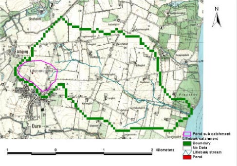
Figure 3.3 Pond location in Lillebæk catchment.
Figur 3.3 Placering af vandhul i Lillebæk-oplandet.
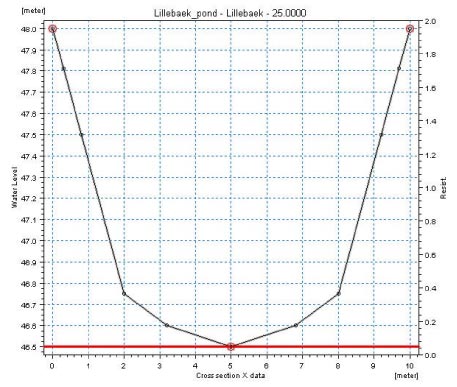
Figure 3.4 Pond cross-section in MIKE 11 for the Lillebæk pond scenario.
Figur 3.4 Tværsnit af Lillebæk-scenarie-vandhullet i MIKE 11-modellen.
Flow into the pond in this catchment consists of drain flow alone. Moreover no recharge from the aquifer will occur as groundwater levels are between 2-3 m below ground surface throughout the year. An area around the pond of app. 0.12 km² was assumed to contribute to the pond with drain flow when groundwater levels are higher than 1.5 m below ground elevation. The drain areas contributing with flow into the pond are delineated in Figure 3.5. The groundwater levels at the subcatchment boundary were extracted from the regional Lillebæk model in order to capture the dynamics and groundwater levels correctly. This also ensures that drain flow into the pond will be limited to the wet season from October to May.
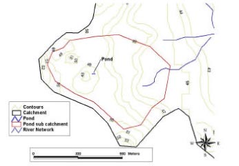
Figure 3.5 Catchment area for Lillebæk scenario pond. Note that only part of the area drains towards the pond.
Figur 3.5 Oplandsareal til Lillebæk scenarie-vandhul. Bemærk at kun en del af arealet dræner mod vandhullet.
In order to maintain a minimum water level in the lake of 0.5 m, the leakage coefficient of the pond bottom lining was adjusted to a value of 5 . 10-7 sec-1.
The water level variation in the pond and inflow to the pond in 1990 is illustrated in Figure 3.6. The pond is surface water controlled as illustrated by the very dynamic inflows to the pond.
Figure 3.6 Simulated pond water level (m) and inflow to pond (m³/s)i Lillebæk scenario.
Figur 3.6 Simuleret vandniveau (m) i og tilstrømning (m³/s) til Lillebæk-scenarie-vandhul.
3.3.8 Implementation of the pond in the Odder Bæk model setup
The pond model for Odder Bæk was set up for the subcatchment area in Figure 3.7. The same grid size of 25 X 25 m² used for the pond in Lillebæk was used for the Odder Bæk pond model.
The pond was set up in MIKE 11 the same way the Lillebæk pond was modelled. The pond size is somewhat larger app. 400 m², which was set up by defining a 40 meter branch and cross-sections similar to the ones used for Lillebæk. Ground elevation is 24.25 m at the location of the pond and the pond was assumed to be 1.5 m deep. Water is assumed to leave the pond through an outlet but may also infiltrate through the lake bottom to the lower layers. The outlet for Odder Bæk pond was modeled by adding a weir to the branch with a crest elevation of 24 m allowing for water to leave the pond before the water level reaches ground elevation.
Figure 3.7 Pond location in Odder bæk catchment.
Figur 3.7 Placering af vandhul i Odder bæk-oplandet.
Flow into the pond in this catchment consists of groundwater flow alone. The topsoil is coarse so water will infiltrate rather than run off on the surface and the groundwater table is close to the surface during the wet season. The groundwater levels at the sub-catchment boundary were extracted from the regional Odder Bæk model in order to capture the dynamics and groundwater levels correctly. A similar water level variation is expected to occur in the pond assuming the pond and underlying aquifer is in contact.
In order to maintain a minimum water level in the lake of 0.5 m and model the groundwater controlled water level variation in the pond, the leakage coefficient of the pond bottom lining was adjusted to a value of 5 . 10-6 sec-1.
The water level variation in the pond and inflow to the pond in 1995 is illustrated in Figure 3.8. The pond is groundwater controlled as illustrated by the simulated in- and outflows for the pond.
Figure 3.8 Simulated pond water level (m) and groundwater exchange (m³/s) in the Odder Bæk scenario pond.
Figur 3.8 Simuleret vandniveau og grundvandsudveksling i Odder Bæk scenarie-vandhullet.
4 Parameterisation of Sub-components
4.1 Growth curves and deposition on soils
4.2 Wind drift
4.3 Dry deposition
4.4 Calculation of effective pesticide dose on the soil
4.5 Adsorption to macrophytes
4.6 Adsorption to suspended matter
4.7 Sediment in streams and ponds
4.1 Growth curves and deposition on soils
Plant growth information appears in the model in two ways. Information on root depth and leaf area index over time determines the calculation of transpiration. Furthermore, the growth stage and percentage cover at a given time determines the amount of deposition on the soil surface. For the calibration of the water model, values from (Plauborg and Olesen, 1991) for the agricultural crops were used for Leaf Area Index and Rooting Depth. For deposition of pesticide on soil, the results from Jensen and Spliid (2003) are used for vinter wheat, spring barley, potatoes and sugar beets. For other crops, the recommendations by FOCUS (2000) are used. Tables illustrating these relationships are given in Appendix B.
Figure 4.1-Figure 4.4 compares the values of Jensen and Spliid (2003) and FOCUS(2000) for the four crops where both data sets are available.
Figure 4.1 Deposition of pesticide on soil under winter wheat, as estimated by Jensen & Spliid (2003) and FOCUS (2000).
Figur 4.1 Deposition af pesticid på jorden under vinterhvede, bestemt af Jensen & Spliid (2003) og FOCUS (2000).
Figure 4.2 Deposition of pesticide on soil under spring barley, as estimated by Jensen & Spliid (2003) and FOCUS (2000).
Figur 4.2 Deposition af pesticid på jorden under vårbyg, bestemt af Jensen & Spliid (2003) og FOCUS (2000).
Figure 4.3 Deposition on soil under sugar beet, as estimated by Jensen & Spliid (2003) and FOCUS (2000).
Figur 4.3 Deposition af pesticid på jorden under sukkerroer, bestemt af Jensen & Spliid (2003) og FOCUS (2000).
Figure 4.4 Deposition under potatoes, as estimated by Jensen & Spliid (2003) and FOCUS (2000).
Figur 4.4 Deposition af pesticid på jorden under kartofler, bestemt af Jensen & Spliid (2003) og FOCUS (2000).
4.2 Wind drift
At present, the Ganzelmeier values for drift are used in Denmark when determining the size of buffer zones required in pesticide registration (BBA, 2000). The values are based on drift experiments carried out in Germany under wind speeds that are common for the continental climate. These wind speeds are relatively low (ca 2 m/s in average for field crops). The Ganzelmeier values are 95% percentile values of individual observations. This means that 95% of the individual measurements have resultet in drift values less than the Ganzelmeier values, which are 2-3 times higher than the average values. The Ganzelmeier values are thus kind of worst case values for the specified wind conditions.
In order to investigate the 2 m/s-assumption, average wind speeds data from the Danish research station “Flakkebjerg” were investigated. Figure 4.5 shows the wind profile over the day, based on average values from May and June, 1991 to 2000.
Figure 4.5 Wind profile at Flakkebjerg research station, average values for the months may and June (1991-2000). The values at 10 m's height are measured, while the speed at 2 m's height is calculated. The low velocities during the night are typical of a coastal climate.
Figur 4.5 Vindprofil på Flakkebjerg forsøgsstation, gennemsnitlige værdiger for månderne maj og june (1991-2000). Værdierne i 10 m's højde er målte mens hastigheden i 2 m's højde er beregnet. De lave værdier målt om natten er typiske for et kystklima.
It is quite common that farmers spray very early in the morning, but even here, the average wind speed is higher than 2 m/s. Assuming that the drift increases linearly with the wind velocity at velocities above 1 m/s. Spraying at wind velocities of 3-4 m/s will result in drift values which, in average, are at the level og the Ganzelmeier values. The figure shows that wind velocities of 3-4 m/s are close to the actual average values found in Denmark during the spraying period in spring.
A careful farmer will be able to carry out his sprayings under more favourable wind conditions, particularly sprayings where the timing is less critical and may take place within an interval of perhaps a week. For many sprayings, however, the timing is critical and only allows spraying within an interval of few days, or alternatively a higher dosage is required.
It was therefore agreed to interpret the Ganzelmeier 95 percentile values as average values for Danish conditions. In the FOCUS surface water scenarios, a special procedure is used for wind drift if more than one application of pesticide is carried out because the drift calculation is interpreted as a 90 % percentile. Such a procedure is not implemented here, as the percentile is interpreted as the average condition.
In the scenarios, the wind is always blowing perpendicular to the stream. This issue was discussed at length. This assumption is an overestimation compared to the general situation, but not necessarily to the conditions during a single spraying event.
Relationships were established between drift and distance from the stream for agricultural crops, apple trees and pine trees. These are based on the Ganzelmeier values, but interpreted as average conditions. An example of this is shown in Figure 4.6. All relations used are described in Appendix C. Winddrift is added over a period of 30 minutes for the whole catchment.
Figure 4.6 Fitted and measured relationship between distance from sprayer and drift applied for agricultural crops.
Figur 4.6 Beregnet og målt sammenhæng mellem afstand og drift anvendt for landbrugsafgrøder.
The input to the stream attributable to spray drift and dry deposition is dependent on the width of the buffer zones. In addition a considerable part of the catchment has natural boundaries against wind drift, which mainly consists of areas that are too wet to be used for cropping. In the part of the catchment where such natural buffer zones exist, they are included in the model. For the Lillebæk catchment, the “piped” part of the stream which appears open in the registration model, has cropping all the way to the edge. Table 4.1 and Table 4.2 show the width of the natural buffer strips at a number of measured points along the stream in the two catchments.
To estimate the input of pesticides to the stream from dry deposition and spray drift it was, as mentioned, assumed that the wind blows perpendicular to the stream. However, it is not reasonable to assume that the wind blows perpendicular along the entire stretch of the streams due to the twists and turns of the streams. To overcome this the effective stream stretch exposed to spray drift and dry deposition was calculated on the basis of a straight line between the start and the end of the modeled open part of the streams in each catchment. Then, stretches of the streams characterized by a uniform width of the buffer zones (Table 4.1 and Table 4.2) were projected onto the straight line whereby the effective length exposed to spray drift and dry deposition was calculated. The positions of the stretches along Odder Bæk and Lillebæk and how the effective exposed length of each stretch is estimated is illustrated on Figure 4.7 and Figure 4.8 respectively. The length of the stream in the model and the exposed length of each stretch in Odder Bæk and Lillebæk appear from Table 4.1 and Table 4.2 respectively.
Table 4.1 Measured width of natural buffer strips along Odder Bæk at different points, divided in to stretches of uniform width, the length of the stretches in the model (chainage) and the exposed (projected) length of the stretches. The measuring points were given with coordinates only.
Tabel 4.1 Målt bredde af de naturlige bufferzoner langs med Odder Bæk , inddelt i strækninger med ensartet bredde, tilhørende længde i modellen og projiceret længde. Målepunkterne var kun opgivet med koordinater.
| Measuring Point | Measured width [m] | Stretch | ||||
| Left | Right | Number | Interpreted width [m] |
Length in model [m] |
Exposed length [m] |
|
| 1 | >20 | >20 | 5 | 20 | 608 | 400 |
| 2 | >20 | >20 | ||||
| 3 | >20 | >20 | ||||
| 4 | >20 | >20 | ||||
| 5 | 0 | >20 | 4 | 0 | 494 | 410 |
| 6 | 0 | >20 | ||||
| 7 | 2 | >20 | ||||
| 8 | >20 | >20 | 3 | 20 | 1267 | 1170 |
| 9 | >20 | >20 | ||||
| 10 | >20 | >20 | ||||
| 11 | >20 | >20 | ||||
| 12 | >20 | >20 | ||||
| 13 | >20 | >20 | ||||
| 14 | >20 | >20 | ||||
| 15 | >20 | 4 | 2 | 0 | 1805 | 1610 |
| 16 | 0 | 4 | ||||
| 17 | 0 | 5 | ||||
| 18 | 0 | 5 | ||||
| 19 | 0 | 5 | ||||
| 20 | >20 | >20 | 1 | 20 | 320 | 320 |
| 21 | >20 | >20 | ||||
Table 4.2 Measured width of natural buffer strips along Lillebæk divided in to stretches of uniform width, the length of the stretch in the model (chainage) and the exposed length of the stretches.
Tabel 4.2 Målt bredde af naturlige bufferzoner langs Lillebæk, inddelt i strækninger med ensartet bredde, tilhørende længde i modellen og projiceret længde.
| Length of stretch from outlet, m |
Measured width [m] | Stretch | ||||
| Left | Right | Number | Interpreted width [m] |
Length in model [m] |
Exposed length [m] |
|
| 70 | 0 | >20 | 5 | 0 | 451 | 440 |
| 130 | 12 | 9.8 | ||||
| 190 | >20 | 1.25 | ||||
| 250 | 11.6 | 0.7 | ||||
| 310 | 9.7 | 3 | ||||
| 370 | 1 | 1.7 | ||||
| 430 | 3 | 1.05 | ||||
| 490 | 13 | 0.75 | 4 | 3 | 183 | 180 |
| 550 | 10.5 | 1.9 | ||||
| 610 | >20 | >20 | ||||
| 670 | >20 | 3 | ||||
| 730 | >20 | 10 | 3 | 10 | 211 | 230 |
| 790 | 10.75 | >20 | ||||
| 850 | 13 | >20 | ||||
| 910 | >20 | >20 | ||||
| 970 | 2.1 | >20 | 2 | 20 | 390 | 230 |
| 1030 | >20 | >20 | ||||
| 1090 | 3 | >20 | ||||
| 1150 | >20 | >20 | ||||
| 1210 | >20 | 18 | ||||
| Not relevant – opened piped stretch | 1 | 0 | 1700 | 1540 | ||
To calculate the input from spray drift and dry deposition according to Asman, Jørgensen and Jensen (2003) one also need to know the width and the length of the fields to which the pesticide is applied. To obtain an estimate of the width of the fields it was assumed that the fields are of equal width at each side of the stream. Furthermore it was assumed that the total area of the fields should be equal to the area of the catchments minus the area found upstream to the upper ends of the open part of the streams. The later is a consequence of the fact that it is impossible that pesticide applied upstream to the open part of the stream enters the stream when the wind blows perpendicular to the stream. The areas of each catchment from which spray drift and dry deposition to the stream can occur, was then calculated from the length of the exposed open part of the stream and the entire length of the catchment. The length of the catchments was determined from an extension of the straight lines between the start and the end of the modeled open part of the stream (Figure 4.7 and Figure 4.8). Hence 77% and 85% of the total area of Odder Bæk and Lillebæk catchment respectively can give rise to input of pesticides attributable to spray drift and or wind drift. The area of the catchments is 11.4 km² and 4.4 km² for Odder Bæk and Lillebæk respectively (Styczen et al 2004a). Hence the width of the fields, of each side of the streams was thus estimated as 1125 m and 715 m for Odder Bæk and Lillebæk respectively. The exposed length of the fields is equal to the length of each water stretch, exposed to wind drift and dry deposition.
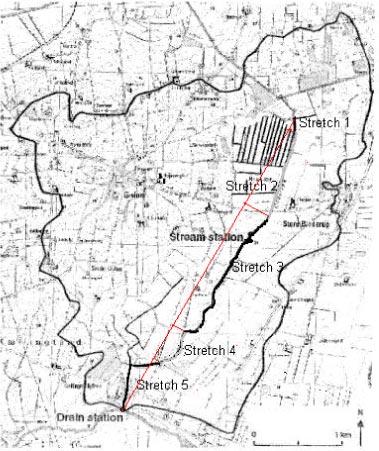
Figure 4.7 The Odder Bæk catchment with indications of stretches and lengths used for drift calculations.
Figur 4.7 Odder Bæk-oplandet med angivelse af strækninger og længder anvendt til drift-beregninger.
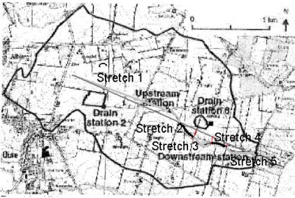
Figure 4.8 The Lillebæk catchment with indications of stretches and lengths used for drift calculations.
Figur 4.8 Lillebæk-oplandet med angivelse af strækninger og længder anvendt til drift-beregninger.
It is possible to specify width of buffer zones in the interface to the model. These values only overrule the existing buffer zones if the value is larger than the existing buffer zone.
For the pond scenarios, the logic applied for the calculations is different. Winddrift is calculated as if the ponds were square, that is 20 * 20 m² for Odder Bæk and approximately 15.8 * 15.8 m² for Lillebæk. The exposed length is therefore 20 and 15.8 m respectively. The calculation of drift is integrated over the width of the pond.
4.3 Dry deposition
The simulation of dry deposition takes place with a model “outside” the MIKE SHE/MIKE 11 model system. The model used is described in Asman et al. (2003) and in the technical documentation (Styczen et al., 2004c). An example of an input file for calculation is shown in Table 4.3. In the table is described how the parameters used are generated. The values either stem from the user interface, are pre-calculated such as information about water body cross sections and width of upland and organic matter content of the soil, or are generated from the MIKE 11 or MIKE SHE water simulations.
With respect to dry deposition, the outstanding question was the size of the agricultural area upwind of the pond. It was decided that it was not reasonable to determine the length of the upwind area based on the hydrological catchment to the pond. Also, it was unreasonable to let the upwind area depend on where in the catchment the site for the pond was selected. It was finally chosen to use the same upwind length for the ponds as has been used for the stream in the respective area.
Due to the fact that the module requires certain values from the water simulations of MIKE 11 and MIKE SHE, the model is executed after the water simulations are carried out and before the solute transport is calculated. In this way, the necessary stream flow parameters can be extracted from the result files and used for the simulation of dry deposition.
Table 4.3 Overview of input to the dry deposition model and the sources of information used for parameterisation.
Tabel 4.3 Oversigt over input til tørdepositionsmodellen, og kilderne til den anvendte parameterisering.
4.4 Calculation of effective pesticide dose on the soil
The input to the soil surface depends on the sprayed dosage and the processes described in 4.1 – 4.3. The pesticide dosage specified in the input file is modified in the following manner:
- If no plants are present on the field, the amount of drift is calculated, and the amounts of dry deposition on the stream and buffer zones are calculated. The total amount is deducted from the total sprayed amount, and the result is divided by the sprayed area. This figure is the input to the unsaturated zone. Emission from and re-deposition to the soil surface is not taken into account.
- If plants are present, the emission of pesticide of relevance for dry deposition is expected to stem from the leaf surfaces. The dosage reaching the soil is therefore only regulated according to the deposition figures by Jensen and Spliid (2003) and for wind drift.
All parameters from the calibrated model relating to transport in the root zone are used directly in the scenario-models. These parameters are described in Styczen et al. (2004a).
4.5 Adsorption to macrophytes
The parameterisation of the sorption to macrophytes included two step. First a Kd value for the sorption to macrophytes was calculated on the basis of an empirical relationship between water solubility and Kd values for different macrophytes and pesticides (1) derived by Crum et al. (1999).
log(Kd) = 3.2 – 0.65 log(S), (1)
where
S denotes the water solubility (mg/l).
Furthermore, it was assumed that the ratio between the sorption and desorption rates is given by the Kd value and that sorption rate is compound and sorbant independent and therefore similar to the sorption rate estimated for the sorption experiments with stream and pond sediments.
The biomass of macrophytes in the stream scenario was estimated on the basis of information from the literature of the yearly succession in the biomass of macrophytes in Danish streams not covered by forest (Sand-Jensen and Lindegaard, 1996). To take the effect of forest cover into account the fraction of the streams covered by forest was therefore estimated by visual inspections along the streams as 0% for Odder Bæk and 50% for Lillebæk. It was then assumed that no macrophytes was present where the stream is covered by forest and the biomass shown on Figure 4.9 was thus multiplied with 0.5 for Lillebæk and 1 for Odder Bæk. The conversion from the unit of g m-2 shown on Figure 4.9 to the unit of g*m-3 used in the model thus assumed an average depth of 0.10 m for Lillebæk and 0.5 m for Odder Bæk respectively.
Figure 4.9 Macrophyte biomass in light open streams
Figur 4.9 Makrofyt-biomasse i lyseksponerede åbne vandløb.
According to the scenario definitions the ponds can be either phytoplankton or macrophyte dominated. These choices are based on a fundamental ecological classification of small Danish lakes, which is illustrated on Figure 4.10. It is the intention that the suite of scenarios together should reflect these classification. Hence the scenarios of macrophyte dominated ponds are supposed to mimic ponds with high density of submerged macrophytes classified as oligortrophic to mesotrophic on Figure 4.10, whereas the phytoplankton dominated scenario is supposed to mimic hypereutrophic conditions. The most oligotrophic conditions are generally found in lakes in sandy catchments and it was therefore decided to let the pond of Odder Bæk be an image of this. Hence the concentration of macrophytes in the pond of Odder Bæk was set to 50 g/m³ corresponding to the biomass of macrophytes to the very left at Figure 4.10.
Figure 4.10 General changes in the balance between phytoplankton, submerged vegetation and floating vegetation and reed swamp along eutrophication gradient.
Figur 4.10 Generelle ændringer i balancen mellem fytoplankton, vanddækket vegetation og flydende vegetation og rørsump som funktion af eutrofiering.
The lakes of the eastern part of Denmark is naturally more eutrophicated than the lakes of the western part. To take this into account the concentration of macrophytes in the macrophyte dominated pond of Lillebæk was set to 700 g/m² corresponding to a biomass of up to 200 to 700 g/m² reported for dense populations of submerged macrophytes in Danish lakes (Jensen og Lindegaard, 1996). Hence, the dense macrophyte populations of the ponds of Lillebæk might reflect both natural and anthropogenic eutrophication.
4.6 Adsorption to suspended matter
Even for active substances with a high Kd for adsorption to suspended matter most of the active substance is found as dissolved substance in the water column. For instance, for the active substance pendimetahlin, with a Kd value as high as 640 l kg-1 only 6 % of the mass will be sorbed at equilibrium at a particle concentration as high as 100 mg l-1. Sorption to suspended matter in the water column was therefore not considered as important in the model. The particle concentration in streams and ponds was therefore given by the amount of particles transported from the catchment into the streams and ponds through macropore flow. Hence, no attempts to adjust for the production of particles in the ponds and streams were made.
4.7 Sediment in streams and ponds
In the streams an upper sediment layer of a thickness of about 2 cm is built up during the summer season and subsequently removed during flood events in the winter season (Iversen et al., 2003). Compared to the lower more crude sediment the content of organic matter in this upper sediment layer is high. Since the extent of sorption of pesticide to sediment particles mainly is related to the content of organic matter only the upper few cm of newly settled sediment is supposed to be of significance for the fate and transport of pesticides in the streams. The thickness of the sediment was therefore set to 2 cm. The porosity of the sediments and the content of organic matter, which is needed for description of the biodegradation, the diffusion and the sorption were reported by Helweg et al. (2003) and appear from Table 4.4.
Table 4.4 Porosity and organic content of the sediment of the different scenaria
| Scenario | Loss of ignition (g/kg d.w.) |
Porosity |
| Lillebæk pond – macrophyt dom. | 82 | 0.75 |
| Lillebæk pond – phytoplan. dom. | 600 | 0.95 |
| Lillebæk stream | 25 | 0.75 |
| Odder Bæk pond – macrophyt dom. | 82 | 0.75 |
| Odder Bæk pond – phytoplan. dom. | 600 | 0.95 |
| Odder Bæk stream | 197 | 0.75 |
For the macrophyte dominated pond the porosity of the sediments and the content of organic matter was set equal to the measurements from the artificial ponds at NERI in Roskilde. The sediment of the phytoplankton dominated ponds is supposed to be very high in organic content, since the scenario is supposed to mimic hypereutrophic ponds with a high production of phytoplankton, which is sedimentating in the pond. The content of organic matter was therefore set to 60% corresponding to the highest loss of ignitions measured for 15 Danish lakes with a high content of organic matter in the sediments. Furthermore the porosity was set to 0.95 reflecting the high water content of sediments rich in organic matter (Miljøstyrelsen 1991).
As a consequence of the high content of organic matter long periods with anoxic conditions in the sediment might frequently be found in such ponds. When the biodegradation was parameterized for the phytoplankton dominated ponds it was therefore assumed that the biodegradation is anaerobic.
We are aware of that the attempt to summarize the ecological conditions in streams and ponds in terms of the selected scenario is a crude generalisation of the complex ecological condition of such systems. This consquences of this is discussed further in Section 7.1.
5 General Conditions for the Simulations
5.1 Simulation Period
5.2 Time Steps of the Simulations
5.3 Initial Conditions
5.1 Simulation Period
It was initially expected to simulate a 10-year period. However, due to problems with the size of the pre-calculated files with results of the water simulations, the simulation period was reduced to four years.
The selected years are 1994, 1995, 1992 and 1997 for Lillebæk and 1998, 1999, 1990 and 1997 for Odder Bæk.
For Odder Bæk, 1998 has an average spring, a wet autumn, 1999 has a wet spring and an average autum. The result is a long wet winter, favouring leaching. 1990 is an average year all through. 1997 is a dry year, which is required to bring the total water balance back to what it is for the 10-year period as such. In all, for the four years, the precipitation minus the actual evaporation is about 19 mm above the average value for the 10-year period.
Table 5.1 Accumulated values of rainfall minus actual evaporation for Odder Bæk for the years 1990 to 2000. The values are accumulated over the specified period and ranked. `= 1990, * = 1997, # = 1998 and ¤= 1999. The boxed values in the middle of the table are the average value for the total period.
Tabel 5.1 Akkumulerede værdier af nedbør minus aktuel fordampning for Odder Bæk for årene 1990-2000. Værdierne er akkumulerede over de specificerede perioder og sorteret efter størrelse. `= 1990, *=1997, # = 1998 og ¤= 1999. De indrammede værdier i midten af tabellen er gennemsnittet for hele perioden.
| Jan-Mar | Jan-Apr | Sept-Dec | Oct-Dec | Year |
| 38 | -8 | 164 | 120* | 130 |
| 104* | 90* | 164¤ | 137 | 131* |
| 126 | 141 | 165 | 146 | 202 |
| 143 | 141 | 176* | 148 | 232 |
| 168 | 164' | 192 | 176' | 272 |
| 179 | 195# | 286 | ||
| 199 | ||||
| 172 | 181 | 204 | 177 | 293 |
| 190' | 194 | 224 | 178 | 295' |
| 196# | 243# | 235' | 183¤ | 397¤ |
| 202 | 260¤ | 235 | 199# | 418 |
| 217¤ | 281 | 298 | 201 | 425# |
| 243 | 302 | 221 | 435 | |
| 265 | 242 |
Table 5.1 shows how the selected years compare to other years. It was attempted to ensure that two values were above average and two were below average for each analysed period. Although this was not fulfilled for all periods, the resulting combination was the best that could be obtained.
The same sort of logic has been tried implemented for Lillebæk Table 5.2. 1994 is a very wet year, particularly with a wet spring but also with a wet period in September. The winter 1994- 1995 is a continuous period with high percolation. 1992 is close to average, while 1997 is a dry year. The distribution of dry and wet years is such that for each of the analysed periods, two are above and two are below average, except for the yearly totals, where two is below, one is average and one is above the average value. The average value for the four years is 16 mm above the average for 1990-2000.
Table 5.2 Accumulated values of rainfall for Lillebæk for the years 1990 to 2000. The values are accumulated over the specified periods and ranked. ' = 1992, ¤ = 1994, # = 1995 and * = 1997. The boxed values in the middle of the table are the average value for the total period.
Tabel 5.2 Akkumulerede værdier af nedbør for Lillebæk for årene 1990-2000. Værdierne er akkumulerede over de angivne perioder og sorteret efter størrelse. ' = 1992, ¤ = 1994, # = 1995 og * = 1997. De indrammede værdier midt i tabellen er de gennemsnitlige værdier for hele perioden.
| Jan-Mar | Jan-Apr | Sep-Dec | Oct-Dec | Year |
| 81 | 113 | 140# | 128# | 626 |
| 134* | 180* | 236 | 190 | 663* |
| 207' | 249 | 255 | 209* | 679 |
| 218 | 258 | 275* | 224 | 805 |
| 218 | 279 | 313 | 239 | 819# |
| 245 | 304' | 246 | 820 | |
| 849' | ||||
| 266 | 326 | 319 | 248 | 853 |
| 289 | 329 | 325 | 284' | 925 |
| 328 | 394 | 366 | 291¤ | 1023 |
| 354 | 425 | 367 | 296 | 1030 |
| 402¤ | 524¤ | 388 | 299 | 1145¤ |
| 455# | 532# | 405' | 326 | |
| 438¤ |
Table 5.2 shows how the selected years for Lillebæk compare to other years. Also the recharge to groundwater and the drain flow was analysed. This is shown in Table 5.3.
Table 5.3 Ranking of yearly flows from drain to stream and recharge to groundwater. The asterisks indicate the selected years.
Tabel 5.3 Sorterede værdier af årlige afstrømninger fra dræn til å og nedsivning til grundvand. Stjernerne indikerer de udvalgte år.
| drain to stream | Recharge to groundwater | |||
| 94 | *511 | 94 | *655 | |
| 95 | *438 | 98 | 533 | |
| 99 | 362 | 95 | *478 | |
| 98 | 329 | 99 | 446 | |
| 93 | 301 | 93 | 420 | |
| 92 | *404 | |||
| 90 | 385 | |||
| average | 282 | average | 379 | |
| 90 | 261 | 91 | 308 | |
| 92 | *259 | 89 | 223 | |
| 91 | 246 | 97 | *176 | |
| 89 | 189 | 96 | 143 | |
| 97 | *122 | |||
| 96 | 89 |
One particular event in the September 1994 – included in the Lillebaek-simulations as 1994 and 1998 requires particular attention. On the 16th and 17th September, 56.6 mm and 18.5 mm of rain falls in the scenario. These values are found in other rainfall records from Funen as well, and are as such realistic. However, such values do not occur very often. For the 24-hour rainfall the value equals a 10 year-occurrence and for the combined 48-hour-rainfall, it equals a one in 20 year-occurrence. These values are derived according to the recommendations given by Spildevandskomiteen and the appropriate excel-sheets can be found on http://www.er.dtu.dk/projects/svk26/.
The same four years are used as a warming up period for the solute transport calculations, resulting in an 8-year simulation of solute transport. The evaluation may be done on the last four years.
NB- due to the fact that the warming up period in Lillebæk is one day too short, the dates for the last four years are wrong by one day. It has been ensured that all files are compatible, but it means that when spraying takes place on eg. 1.5, it appears in the result files on 30.4 for the last four years.
5.2 Time Steps of the Simulations
Time steps vary over the different parts of the model. During the water simulation, the models adjust their internal time steps to the conditions, and during rainfall events, the models may calculate in fractions of seconds. However, due to the approach chosen, where the water files are produced and stored, and the solute transport is implemented based on the stored flows, there is a certain averaging taking place in the model. The MIKE 11 water movement is stored every 60 minutes, and the level of detail in this part of the model therefore lives up to the original expectations. Wind drift and deposition will therefore be simulated as “instant” concentrations.
With respect to the storing steps in MIKE SHE, there was a considerable conflict between the length of the simulation period and the preferred storing frequency. The following steps were taken to overcome the problem:
- The reading and writing routines of MIKE SHE were rewritten to zip the information while writing,
- Drainage flows are now stored in MIKE SHE at the same frequency as overland flow, and not, as before as groundwater,
- The simulation period has been reduced from 10 years to 4 years to minimize the period required with detailed storing in MIKE SHE.
- Investigations were made to find a way to avoid the approx. 4 Gigabytes limit for one file in the Windows system. By formatting the disks as NTFS, larger files can be generated. However, it was not, in the time of the project, possible to make the solute transport programme accept the large files. There may be ways around this problem with specialised compilers, but the time did not allow further investigations.
- External files of 160 Gigabytes with FireWire connection were bought to the project with the purpose of storing MIKE SHE water movement files and handing them over to the Danish EPA.
The final storage frequency of water movement information in for Odder Bæk stream and pond is as follows:
- 2 hours on the overland flow and drainage components,
- 24 hours in the unsaturated zone, and
- 24 hours in the saturated zone
The calculation time steps are maximum 2 hours for the overland and unsaturated zone components, and maximum 6 hours for the saturated zone. The internal MIKE 11 timestep is 3 minute. However, no more than 0.5 mm rain is allowed within a timestep.
For the Lillebæk scenario, the storing frequency is 4 hours for the overland flow and drainage component, 16 hours for the unsaturated zone and 48 hours for the saturated zone. The calculation time step are maximum one hour for the overland flow and saturated zone-components and 6 hours for the saturated zone. The timestep for MIKE 11 is 3 minutes. Maximum 1 mm of rain is allowed in a timestep.
The storing frequency is considered too low to obtain optimal results from the simulations. To improve the quality of data it is necessary either
- to break the limit of approximately 4.2 Gigabytes in one file,
- to change the output file system of MIKE SHE so the result files are split up, or
- to run the water and solute simulation together to avoid the intermediate files. This last solution will, however, require considerable code changes and will make the simulations very slow.
The first solution may be technically possible, while the second definitely is. It does, however, require some re-coding.
The internal time step of the solute transport calculation is regulated to ensure model stability. The results of the solute transport calculation in MIKE 11 are stored with variable frequency. During the first two hours after spraying, values are stored every 10 minutes. For the next 30 days, data are stored hourly. The rest of the period, data are stored every third day. These files are used for the output programme. MIKE 11 can store the results with much larger frequency, but the result presentation programme cannot read the data.
Solute transport is stored every 30 days in MIKE SHE, where it is only used for generation of monthly and yearly solute balances.
5.3 Initial Conditions
The initial conditions for the model stem from the original model. No solute is present in the system at the beginning of the simulation. However, with the four years warming-up period, it is expected that the system has warmed up sufficiently, and that pesticide concentrations in the stream can be used for analysis after this time.
6 Mass Balances of Scenarios
6.1 Water balances
6.2 Solute balance examples
6.1 Water balances
The water balances are fixed for each scenario, as the water files have been prepared in advance. The summarised water balances are included in the tables below. The monthly water balances for the full runs are shown in Appendix E. Due to the fact that the actual time steps used in the model are not completely identical, there are small differences between the precipitation sums in the balances.
It is seen that surface runoff is negligible for all scenarios. There are differences between the scenarios due to the crop choice, but they are small.
Click here to see Table 6.1 – 6.8.
Table 6.1 Average monthly waterbalance for Odder Bæk pond, when the catchment is cropped with spring barley.
Tabel 6.1 Gennemsnitlig månedlig vandbalance for Odder vandhul, når oplandet dyrkes med vårbyg.
Table 6.2 Average monthly waterbalance for Odder Bæk pond, when the catchment is cropped with winter barley.
Tabel 6.2 Gennemsnitlig månedlig vandbalance for Odder vandhul, når oplandet dyrkes med vinterhvede.
Table 6.3 Average monthly waterbalance for Odder Bæk, when the catchment is cropped with spring barley.
Tabel 6.3 Gennemsnitlig månedlig vandbalance for Odder Bæk, når oplandet dyrkes med vårbyg.
Table 6.4 Average monthly waterbalance for Odder Bæk, when the catchment is cropped with winter wheat.
Tabel 6.4 Gennemsnitlig månedlig vandbalance for Odder Bæk, når oplandet dyrkes med vinterhvede.
Table 6.5 Average monthly waterbalance for Lillebæk pond, when the catchment is cropped with spring barley.
Tabel 6.5 Gennemsnitlig månedlig vandbalance for Lillebæk vandhul, når oplandet dyrkes med vårbyg.
Table 6.6 Average monthly waterbalance for Lillebæk pond, when the catchment is cropped with winter wheat.
Tabel 6.6. Gennemsnitlig månedlig vandbalance for Lillebæk vandhul, når oplandet dyrkes med vinterhvede.
Table 6.7 Average monthly waterbalance for Lillebæk , when the catchment is cropped with spring barley.
Tabel 6.7 Gennemsnitlig månedlig vandbalance for Lillebæk, når oplandet dyrkes med vårbyg.
Table 6.8 Average monthly waterbalance for Lillebæk , when the catchment is cropped with winter wheat.
Tabel 6.8 Gennemsnitlig månedlig vandbalance for Lillebæk, når oplandet dyrkes med vinterhvede.
6.2 Solute balance examples
Simulations were carried out for Substance 2 defined for the FOCUS scenario in order to produce a set of examples. Mass balances were produced in order to show how the substance spreads through the different scenarios. In addition, plots from the different runs are presented.
When comparing with the FOCUS surface water scenarios it should be noted that a very high percentage of the upstream catchment is sprayed in these scenarios, while in the FOCUS surface water scenarios, it is only 20 % of the area. Secondly, for the Lillebæk scenario the peak occurring around the 16th of September 1994 and 1998 is a one in 10-years or one in 20 years-event based on the 24 and 48 hour rainfall alone. Several active substances simulated with the model produce very high peaks on this particular date.
Figure 6.1 to Figure 6.4 show the concentrations along the stream or in the pond. The upper left plot shows the concentrations as a function of time and position along the stream. The plot in the upper right corner shows the highest concentration per event within a 24 hours period along the length of stream. In the lower left is shown a number of time series for selected points along the stream.
The highest concentration obtained in the Odder baek scenario is 1.815µg/l, descending to about 0.5 µg/l after 12 hours. Substance 2 does not seem to have been calculated for the FOCUS D3-stream-scenario, which is most comparable. However, for the D3-ditch, concentrations reach 5.27 µg/l. The Odder pond-scenario reaches 1.6 µg/l at the maximum. The pond overflows from time to time, and due to this, it is to some extent comparable to a stream section.
For Lillebæk, the FOCUS D4-scenario is the most comparable. The prediction of maximum stream concentrations for substance 2 appears to be 3.92 µg/l. It should be taken into account that only 20 % of the upstream catchment is sprayed, meaning that the values from PestSurf is likely to be about 4.5 times higher due to the larger area sprayed. However, the highest concentration recorded is 6.6 µg/l in the downstream end of the catchment and 5.4 µg/l in the top end. The highest event observed occurs on the date with a 20 year-rainfall-event. In the upstream end, it is about a factor 1.5 higher than other events. For the downstream end, other events of the same magnitude are observed.
Compared with the FOCUS-scenarios, the model thus simulates relatively lower concentrations, taking into considerations the assumptions. This is to be expected because the model takes into account a larger degree of variation between fields and drainage conditions.
The Lillebæk pond scenario reaches 3.3 µg/l at the maximum. The pond seldom overflows, and pesticide in the pond tends to stay until it breaks down.
For the shown simulations, breakdown in the groundwater is assumed for Odder pond only. This scenario is not drained, and this assumption leads to groundwater within the upper meter of the soil, for at least part of the year. It is therefore necessary to assume a breakdown in the upper part of the groundwater for this scenario.
It is, however, obvious, that the water bodies over time receive a considerable amount of pesticide through the groundwater. This is a function of the shortcomings of the model described in Styczen et al. (2004a) and of the assumption that no breakdown takes place below 1 m from the surface.
Click here to see Table 6.9 – 6.12.
Table 6.9 Yearly mass balance for substance 2 in the Odder stream scenario in absolute values and percent
Tabel 6.9 Årlig massebalance for substans 2 i Odder bæk-scenariet i absolutte værdier og procent
Table 6.10 Yearly mass balance for Substance 2 in the Odder pond scenario scenario in absolute values and percent
Tabel 6.10 Årlig massebalance for substans 2 i Odder bæk-vandhuls-scenarie i absolutte værdier og i procent.
Table 6.11 Yearly mass balance for Substance 2 in the Lillebæk stream scenario scenario in absolute values and percent.
Tabel 6.11 Årlig massebalance for substans 2 i Lillebæk å-scenariet i absolutte værdier og procent
Table 6.12 Yearly mass balance for Substance 2 in the Lillebæk pond scenario scenario in absolute values and percent.
Tabel 6.12
Click here to see Figure 6.1 – 6.4.
Figure 6.1 Concentrations of substance 2 simuleret in the Odder Bæk stream scenario.
Figur 6.1 Koncentrationer af substans 2 simuleret i Odder Bæk-scenariet
Figure 6.2 Concentrations of substance 2 simuleret in the Odder Bæk pond scenario
Figur 6.2 Koncentrationer af substans 2 simuleret i Odder Bæk-vandhul-scenariet.
Figure 6.3 Concentrations of substance 2 simuleret in the Lillebæk stream scenario a) the upstream part b) the downstream part.
Figur 6.3 Koncentrationer af substans 2 simuleret i Lillebæk-scenariet a) vandløbets øvre del, b) Vandløbets nedre del.
Figure 6.4 Concentrations of substance 2 simuleret in the Lillebæk pond scenario
Figur 6.4 Koncentrationer af substans 2 simuleret i Lillebæk-vandhul-scenariet.
7 Uncertainty Issues in Relation to the Scenarios
7.1 Introduction
7.2 Uncertainties related to model choice and model parameterisation
7.2.1 Colloid transport and macropore representation
7.2.2 Dispersion in the upper part of the groundwater
7.2.3 Effect of storage frequency
7.2.4 Process kinetics
7.2.5 Description of degradation in soil
7.2.6 Diffusion and stratification in ponds
7.3 Uncertainties related to the choice of scenarios
7.4 Uncertainties related to input
7.5 Uncertainties related to the interpretation of output
7.6 Strategies to further reduce the uncertainty
7.1 Introduction
The description of uncertainty follows to the largest possible extent the description given in FOCUS (2002).
The four main types of uncertainty described in this chapter are:
- The uncertainty related to the correctness of the process descriptions within the applied models. Mathematical models necessarily need to simplify the complex processes found in nature for their simulations.
- The uncertainty related to the choice of scenarios for weather, soil and crop. Transport of pesticides is influenced by many factors, and only a limited number of factors were taken into consideration when selecting the scenarios.
- The uncertainty related to the estimation of input for the scenarios. This is to a large extent discussed in Styczen et al. (2004a) with respect to the selected parameterisation of the catchments, but some factors are changed when the models were transformed into scenarios and particularly for the pesticide parameters, the uncertainty is of importance.
- The uncertainty related to the calculation and interpretation of output.
7.2 Uncertainties related to model choice and model parameterisation
If a compound is subject to processes, which are not considered in the model structure, then this will contribute to the modelling error. Three easily understandable examples are
- The erroneous simulation due to a wrong model concept. For instance, the process implemented in the model assumes that the substance degrades according to first order kinetics, but the degradation of a substance does not follow this kinetics.
- The ignorance of a process relevant for the behaviour of the substance. For instance, a volatile chemical is simulated with a model not accounting for volatilisation,
- The erroneous simulation due to a biased model concept. For instance leaching in a structure soil is simulated with a model that accounts for chromatographic leaching only.
7.2.1 Colloid transport and macropore representation
The calibration of the catchment models show that there are problems with certain process descriptions. According to Holm et al. (2003), the colloid description applied does not explain the observed transport of strongly sorbing compounds.
The same result was observed when comparing simulated and measured pesticide transport in the Lillebæk catchment. The stronger, the pesticide sorbs, the larger the error. However, this was to a large extent counteracted by an exaggerated simulation of macropore flow caused by the requirements of the colloid-transport description. All in all the transport of pesticide to the groundwater is overestimated in the present representation.
For the Odder Bæk scenario, the original assumption was that the area was very sandy, and therefore not subject to macropore flow and drainflow. The soil types have been changed to what was actually observed and drains were included, but macropores were left out. The calibration exercises have shown that macropores probably are present in the catchment anyway. This is particularly visible because highly sorbing compounds such as pendimethalin are found in the stream. Pendimethalin was measured in the drain in Odder Bæk and 36-46% of the pendimethalin in the sample was sorbed on colloids. Omitting this process thus means that the transport of strongly sorbing compounds is severely underestimated in this scenario. In order to reached the observed pesticide concentrations, the foc-values have been halved (see Styczen et al., 2004a) – this may to some extent compensate for the omission of macropores. However, the measured values for organic matter were unusually high.
7.2.2 Dispersion in the upper part of the groundwater
There are problems with catching the first peaks occurring during autumn, and in general, the transport of pesticide with groundwater appears to be too high.
Drain flow is generated in the upper calculation layer of the saturated zone. Only when the water level raises above the drain level is drain water produced. In reality it is observed that drainflow occurs already before the groundwater level raises due to locally saturated codintions around drain depth. The top layer of the saturated zone is rather deep (3-4 meters) and this causes the leaching from the unsaturated zone to be mixed into too much water. It is, however, not possible to make it smaller, as MIKE SHE requires it to cover the variations in ground water level, and considerable efforts have been put into making this layer as thin as possible.
The high macroporre flow and the problem with catching the fist autum peaks undiluted leads to too much pesticide in baseflow. It is difficult to quantify this error, as some mixing also takes place in natural drainflow. If drainflow is generated from a layer of 0.5 m and the calculation layer is 3.5 m deep, the peaks will either be 1/7th of the correct concentration or, if the peaks are of the right magnitude, the mass moving to groundwater will be 7 times to high. A rough estimate of this error is a factor 5-10.
As it has been agreed early in the project to follow the FOCUS (2000) recommendation with respect to zero degradation of pesticide below one meter, the pesticide can undergo sorption or transport only.However, as the saturated zone from time to time penetrates into the upper meter, the parameterisation of the lower part of the root zone is extended to the first calculation layer of the groundwater zone too.
7.2.3 Effect of storage frequency
The too low peaks are also caused by the storage time steps in the intermediate water result files. Values of flow are averaged over a timestep. However, it has not been possible to increase the storing frequency to the extent wished.
7.2.4 Process kinetics
With respect to process kinetics, there is no doubt that at least for some of the pesticides; the kinetics of their reactions with soil and colloids is of importance. The “standard” MIKE SHE-model is able to handle kinetics of processes, but the choice of process descriptions to be included were limited by the fact that Danish EPA should have access to the data, and the standard input produced by the companies is simple Koc-values or similar. The effect of kinetics is not straight forward. In some cases, a compound may leach faster, because it does not in reality have time to become adsorbed. On the other hand, equilibrium assumptions lead to that all adsorbed pesticide eventually leaves the soil column, while some observations show that sorption may be irreversible for some compounds.
7.2.5 Description of degradation in soil
The data is also a problem with respect to the description of degradation in MIKE SHE. It was attempted in the calibration procedure to calculate leaching with the assumption that adsorbed pesticide breaks down at with the same speed as pesticide in solution, or with the assumption that sorbed pesticide do not break down. The first of these assumptions is usually the one implemented in registration models. However, for some pesticides there may be a difference between the two phases, but this is not visible from the data available to the EPA's for registration. Assuming that pesticid breaks down in solution only, results in leaching over a much larger period and much higher residues in soils.
7.2.6 Diffusion and stratification in ponds
The value of the diffusion coefficient used for the pond model is associated with problems in relation to uncertainty. This is an indirect consequence of the fact that the diffusion into the sediment in many cases only penetrates the sediment in a very thin layer (see Appendix D). The layer thickness can be a range of 1/10 mm. This implies that the effective area of the water column/sediment interface is much larger than the simple cross-section area. One single m² of the bottom surface may have an effective area in the range of 10-100 m² if the surface roughness is taken into account on the length scale of 1/10 mm. This may explain why the diffusion coefficient for sediment transfer is calibrated to be higher than the value for molecular diffusion in the pond experiment (Styczen et al., 2004a and Mogensen et al., 2004). In addition, the effective diffusion coefficient might vary with a factor of at least 10 between two years in the same pond (Styczen et al., 2004a). As a compromise the effective diffusion coefficient in the registration model was set to the average of the diffusion coefficient obtained for the two year. However, it must be emphasised that the variation in effective diffusion coefficients between different ponds and years all over Denmark is not known, and this is a major source to uncertainty. The variability of the molecular diffusion coefficient due to substance specific properties seems limited compared to the factor mentioned above. But, the difference in adsorption characteristics may have a large influence on the sediment uptake by diffusion (see Appendix D).
Experimental studies conducted in the artificical ponds at NERI in Roskilde revealed that a vertical stratification of the pesticides was present within the first hours to day after the addition of a pulse of pesticide. This is not taken in to account by MIKE 11, which only has one vertical layer. In addition, the role of the macrophytes for the verical stratification is not taken in to account. Compared to the overall uncertainties of the model at catchment scale, the above deviations at pond scale is probably of minor importance for the fate and transport of pesticides at large. However, for the interpretation of model results in terms of pesticide exposure and toxicity, the deviation might be important. For instance, high concentrations in the upper part of the water column might give rise to higher concentrations in the surface microlayer, which migh be an important exposure route for some pond organisms.
Hence the importance of the deviation between the model and the “reality” observed by the pond experiments can only be determined through a linking of the fate model to an exposure and effect model.
In the ponds at NERI, Roskilde, the deviations between the model predictions and the measured data was detected through an intensive measurement program in a controlled system and the model for the pond was developed along with the results of these experiments. For instance, the mathematical description of the diffusion into the sediment and the effective diffusion coefficient is a direct result of the interaction between experiments and model. However, for the stream part of the surface water model the interaction between the measurement and the model work was fairly weak. Hence the calibration or verification of the stream model was conducted at catchment scale, where the MIKE SHE model, due to a longer residence time of the pesticides in the soil compartment, mainly determines, the occurrence of the pesticides in the surface water. Many of the processes in the stream have therefore not been been evaluated as intensively as the process for the ponds.
In accordance with the recommendation of the inception report (DHI et al., 1998) different mathematical descriptions of diffusion of active substance in to the sediment bed were applied in the stream and the ponds. However, through the project theoretical consideretations revealed that the choice of a single box approach for description of the diffusion in the streams might be dubios. Data for an experimental evaluation of the approach is, however, not availbable, since the calibration of the stream model was conducted at catchment scale omitting the options for an intensive evaluation of the process descriptions in the stream. The theoretical difference between the box approach applied for the streams and the diffusive approach applied for the ponds appear from Figure 7.1.
Figure 7.1 Ratio between flux of active substance into the sediment estimated by a single box approach and a multi box approach. The one box approach is used for the streams, whereas the multi box approach is used for the ponds.
Figure 7.1 Forholdet mellem optaget af aktivt stof i sedimentet estimeret med et en box og et multi box approach. En box approachet anvendes for vandløbsmodelen medens multibox apporachet anvendes for vandhullerne.
As it appears from Figure 7.1 the flux of active substance into the sediment is much smaller for the one box than for the multi box approach, espcecially at the time scale of less than an hour. Hence the flux of active substance in to the sediment might be underestimated by the one box approach. This might for instance explain why the concentrations in the water column of a highly sorbable compound like pendimethalin tend to be overestimated in Lillebæk stream by the model. Furthermore most of the degradation of active substances might take place in the sediment due to the local high concentration of degrading bacteria, whereby the effect of an underestimation of the flux is further enhanced. Hence an implementation of the multi box approach for description of diffusion into the stream model might be a significant improvement of the model.
7.3 Uncertainties related to the choice of scenarios
The two catchments were selected to represent a moraine clay area and a sandy area. It is, however, extremely difficult to judge the term “representative” in quantitative terms. It has already been described how the selected catchments compare to the rest of Denmark with respect to rainfall, soil types and crops. With respect to all of these parameters, the values fall within the normal range. None of them are extreme. The presence of buffer zones in the Lillebæk scenario may be compared to the study carried out by Syngenta (Hendley et al, presentation given to the Danish EPA at Syngenta) for all of Funen. The study identified that ponds have 49% of their 20 m margin cropped (and 51% not cropped), and 62% of the streams have their 20 m margin cropped. In comparison, the scenario pond in Lillebæk has a minimum buffer zone of 0. The “original” Lillebæk Stream has ((1080-230)/1080=) 79% of the length cropped within its 20 m margin. This appears to be more than the average value. 57% of the length that is cropped within the 10 m-margin. This value becomes somewhat distorted in the scenario as the piped part of the stream is opened and allocated a 0 m buffer zone. This means that 91% of the stream is cropped within its 20 m-zone. In this case, the scenarios are thus likely to overestimate the drift values by a factor of about 1.5.
A similar study does not exist for Northern Jutland, as mentioned earlier, the presence of permanent grass in the catchment is slightly lower than the average value for similar Danish counties.
There are no indications that the geology in the Lillebæk area should be particularly different from other moraine areas. The parameter values used are not extreme for this type of environment. The stream itself is, however, rather steep for Danish conditions. The main problem with Lillebæk as a scenario is that water actually runs into the area from the western side and that there are losses, probably to the south and definitely to the east, towards the Great Belt. This is, as far as possible, taken into account in the model, but there is, of course uncertainty related to the description of geology.
With respect to the Odder Bæk scenario, there are a number of problems related to the description itself. As described in Section 3.2, the catchment turned out to be less sandy than expected and pipe drained in some areas. The effect of the different soil texture in the root zone has been tried out by exchanging the texture over the entire catchment with a JB1 from the Jyndevad research station. Results indicate that discharge in the stream is increased by 11% and in the upstream drain by 17%, mainly due to an increased baseflow from groundwater (Figure 7.2).
Figure 7.2 Discharge in stream and drain at Odder Bæk, simulated with observed texture(a) and with JB1 texture (b), both compared to observed discharges.
Figur 7-2 Afstrømning fra å og dræn ved Odder Bæk, simuleret med observeret textur (a) og med JB1 textur (b), begge sammenlignet med observerede afstrømninger.
With regard to the effect on pesticide concentrations, it is seen from Figure 7.3 that in the situation with JB1 texture, the concentrations in the stream and in the drain are increased by a factor of 2 to 5. This is explained by the fact that the pesticides don’t reside as long time in the active upper soil layers where sorption and degradation is relatively significant, as compared to the case where the soil is more fine-textured. In conclusion, the flux of pesticides in the stream can be expected to increase by a factor of approximately 2 to 5 when the soil is more coarse-textured.
Figure 7.3 Pesticide concentration in stream and drain at Odder Bæk, simulated with observed and JB1 texture, both compared to observations, for bentazon, isoproturon, and terbuthylazin.
Figur 7-3 Pesticidkoncentration i å og dræn ved Odder Bæk, simuleret med observeret og JB1 textur, begge sammenlignet med observerede værdier, for bentazon, isoproturon, og terbuthylazin.
As a result of the problems described in Section 3.2, the fact that validation could not be carried out on the drain in Odder Bæk, and the fact that macropores appear to be present and important, the validation status of the Odder Bæk scenario is judged as poor.
7.4 Uncertainties related to input
The status of the basic inputs is described in Styczen et al., (2004a). The issue of the choice of foc-values has received attention there. The main additional inputs in the scenarios are the pesticide parameters.
The pesticide parameters used for calibration exercise came from the Pate database (The Danish EPA). It was generally very difficult to recalculate the values given to standard values as proposed by FOCUS (2000). This was particularly so for degradation values. Very often, the estimates of half-lives were effectively based on as little as two soil horizons. As these values are known to be very variable, the estimates are considered very uncertain. Estimates of Q10 were sometimes based on one observation only. With respect to sorption, Koc-factors in the database mostly lay within the interval of ±50 % of the average value.
Examples are given in Stycen et al. (2004a) of confidence intervals for pesticide simulations based on the uncertainty of Kd and DT50.
With respect to choice of sorption model, it was stated for several compounds in the database that sorption followed a Freundlich isotherm, but with no supporting information of the value of the exponent. For Bentazon, the dataset included experiments that clearly followed a linear isotherm and experiments that followed a Freundlich isotherm. The units of the Kd-values were not always clear in the database. It was decided in the calibration exercise to use linear isotherms for all compounds, not least because the choice of a Freundlich isotherm strongly increases sorption at the smallest concentrations, leading to very little leaching.
It is recommended that the EPA use linear sorption unless there is very strong evidence to support the choice of a Freundlich isotherm. In that case, it is important that the supporting documentation also has been generated in the concentration range of interest for leaching.
7.5 Uncertainties related to the interpretation of output
As a result of the errors and uncertainties discussed above, there is considerable uncertainty related to the output. There are, however, no expected errors generated by the methods of post-processing.
7.6 Strategies to further reduce the uncertainty
More work is required on the mechanism of generation of pesticide-loaded colloids. The developed description is included in the model, but it does not produce the concentrations observed in the field. The present oversimulation of groundwater concentration could be reduced somewhat by removing the colloid description and reparameterising the macropores.
It would be advantageous to include drain flow from the unsaturated zone in MIKE SHE. It is not an option in the existing model, but it is technically possible. It is expected that this would much improve the simulation of the peak concentrations in drain flow.
Thirdly, it would be advantageous to be able to store larger intermediate files with higher frequency than is presently the case. This could either be done if the 4.2 Giga limit could be broken or by changing the data storage system of MIKE SHE to open new files when the files had reached the maximum value. Alternatively the storage frequency should be made a function of concentration levels, and/or flow rates.
8 Uncertainty Analysis of the Registration Model
8.1 General systematic in uncertainty analysis
8.2 Principle of the uncertainty analysis - intelligent Monte Carlo
8.3 Uncertainty on the quantification of the variance
8.4 Implementation in to the user interface
This chapter sum up the detailed uncertainty evaluation performed in Appendix D. The chapter is complementary to Chapter 7. Hence Chapter 7 covers various aspects of uncertainties with regard to the scenarios and how well the implemented matematical functions describes the condition in the catchments. The aim of the current chapter is to provide an approach for how to cope with the uncertainty or variation associated with the pesticide specific parameters. To facilititate a dicrimination between the uncertainties considered in Chapter 7 and in the present chapter a short general discussion of the various types of uncertainty is provided in Section 8.1.
8.1 General systematic in uncertainty analysis
The uncertainty of the model predictions is crucial when models are applied in decision-making. Some kind of uncertainty estimate is therefore needed before the model system can be said to have predictive power because it is not possible to evaluate a calculated property if no information about the uncertainty exists. However, it is difficult and in practise even impossible to perform complete uncertainty estimates that take all sources of model uncertainty into account. But this does not mean that the model uncertainty cannot be evaluated. The task is to gather as much information as possible about the model uncertainty before the model system is applied.
There exist two principally different sources of uncertainty relating to the predictive model itself:
- Structural uncertainty arising form the assumptions needed for the model equations to describe the phenomenon in question.
- Input parameter uncertainty as a consequence of variability and lack of knowledge.
Methodologies for performing structural and input parameter uncertainty estimates are different. The structural uncertainty can only be truly estimated in cases where the total uncertainty on input parameters is known and the model predictions can be compared with “reality” at the same time. This introduces the need for high quality data to validate the model and will not be a part of this work. It is however important to emphasise that if sufficient data are available to make a complete determination of the structural uncertainty, then data are needed for all possible model outcomes and in these cases there is hardly any need for predictive models for decision making. The structural uncertainty is dealt with in details in Chapter 7 whereas the uncertainty of the pesticide specific input parameters is the topic for the present chapter.
Straightforward methods for quantifying the input uncertainty, point 2, exist, typically by using a Monte Carlo type analysis (see Figure 8.1). But they often involve laborious calculations for larger models such as the registration model. The topic for this part of the work is to set up guidelines in order to make it possible to evaluate model outcome uncertainty of the registration model.
It is important to emphasise that analysis of input uncertainty needs to be done carefully in order not to create false realism. Uncertainty analysis for predictive models is often by itself rather uncertain, where the uncertainty estimates are associated with uncertainty. The uncertainty analysis will tend to underestimate the “true” variability due to the missing of quantification of the structural uncertainty, considered in Chapter 7.
8.2 Principle of the uncertainty analysis – intelligent Monte Carlo
The purpose is to assess the uncertainty of the calculated pesticide concentrations in the stream and pond compartments as a function of the uncertainties on input parameters. A Monte Carlo analysis can be performed as illustrated in Figure 8.1. Repeatedly the model will be run using a random selected value for every input parameter in the analysis and Figure 8.1 shows how to perform one single run. The variability of the modelling result reflects the uncertainty due to pesticide specific input parameters. If all possible input parameters in a large model are going to be investigated using this type of analysis then often an unrealistic large number of model runs are needed. So, a critical aspect is to select a limited number of input parameters for the uncertainty analysis in a way so the major part of the uncertainty is accounted for.
In most cases a single or a few processes, depending on the environmental conditions and the properties of the actual pesticide, will control the modelling result. For the stream/pond part of the model (MIKE 11) simple relationships have been derived to identify such a dominance (Appendix D), which will be helpful in order to focus the uncertainty analysis to a few controlling parameters. In brief the simple relationships consist of a simple version of the MIKE 11 module, which do not take the spatial variation and varying boundary and forcing functions in to account. In addition the differential equations of the model was solved analytical through assumptions of quasi steady state condition in the stream. The result of this analysis is presented as decision tress, which appears from Figure 8.2 to Figure 8.4.
The registration model comprises a soil module (MIKE SHE), which defines the pesticide input concentration to the surface water module (MIKE 11). It have not been possible to derive a simple model for the soil module, MIKE SHE, as for the MIKE 11 module and decision trees for the MIKE SHE part of the model can therefore not be made. The choice of process of relevance for the uncertainty analysis therefore had to be selected through other means. However, the MIKE SHE module only comprises two processes, sorption and degradation, whereas the MIKE 11 module comprises eight processes for which consideration of the uncertainty is relevant. Hence a selection of process seems most relevant for the stream/pond part of the model. Furthermore the calibration exercise (Styczen et al., 2004a) revealed that the concentration in the stream mainly is determined by the process in the MIKE SHE model, which is readily explained the longer residence time of the pesticides in the soil compartment compared to the stream. It was therefore decided always to include the uncertainty of the process, sorption and degradation, of the MIKE-SHE model in the uncertainty analysis.
To reduce the number of model runs further the sampling within a gaussian random field was substituted with a Latin Hyper Cube sampling of Gaussian fields (Pebesma and Heuvelink, 1999).
Figure 8.1 Principles for uncertainty analysis based on Monte Carlo simulations. Input parameters are typically assumed being normal or log-normal distributed. The endpoint is uncertainty estimates on critical stream output parameters.
Figur 8.1. Principper for usikkerhedsanalyse baseret på Monte Carlo-simuleringer. Input parametre forventes at være normal- eller log-normalfordelt. Endepunktet er usikkerhedsestimater på kritiske å-resultat-parametre.
8.3 Uncertainty on the quantification of the variance
To conduct the intelligent Monte Carlo analysis the selected pesticide specific parameters needs to be associated with a standard deviation or variance. In addition the pesticide data from the legislation, stored in the PATE database, will form the basis for the model. These data includes data derived from different laboratories, using different analytical as well as different empirical/statistical models for interpretation of the experiments. To conduct the uncertainty analysis across process on a common basis it is therefore assumed that the experiment is used as the unit of replication when the standard deviation or variance is calculated. In addition is it assumed that the log transformed data follows a normal distribution. The log transformation was needed to avoid a larger numbers of negative estimates of the process parameters.
The uncertainty on input parameters can be then estimated by evaluating the following two topics:
- Uncertainty due to the assumed functional form of the stochastic relationship for input parameter variability.
- Missing information due to the limited number of single data values to estimate the variability of the input parameters.
The type A uncertainty can e.g. be the result of an assumed normal or equal distribution of input data. It has not been possible to evalute whether this assumption is fullfilled on a sound basis, due to a limited number of data. However, a log-normal distribution is frequently used for probabilistic risk assessment and the assumption is thus in line with this practice (Solomon et al 1996, Hall et al., 1996). When the distribution function for the input data is assumed known then the type B uncertainty arises from the fact that the distribution-function parameters (e.g. mean value and variance) needs to be estimated based on a limited number of data values. To overcome point B it is the intention to substitute the log-normal distribution with a t-distribution fitted to the log transformed input data.
8.4 Implementation in to the user interface
Due to logistic constraints caused by the calculation time of the model it is not considered relevant to implement uncertainty analysis in the user interface at the current state. Hence an uncertainty analysis would last for about a month if 25 runs should be conducted as a part of the intelligent Monte Carlo. Instead a spreadsheet deriving relevant input data on the basis of the pesticides properties and the variations thereof have been produced and will be delivered together with the model. In brief the spreadsheet comprise an operationalization of the descision trees through logical (if ..then else..) functions, whereby the input parameters for which the uncertainty is most important for the output of the model is pointed out. The second part of the spread sheet produce 25 sets of input parameters through a Latin Hyper Cube sampling of the selected parameters.
Click here to see Figure 8.2 – 8.4.
Figure 8.2 The decision tree for selecting controlling stream process parameters in relation to the calculated dissolved concentration in the stream.
Figur 8.2 Beslutningsstøtte-træ til selektion af parametre, der kontrollerer å-processer in relation til den beregnede koncentration af opløst stof i vandløbet.
Figure 8.3 The decision three for selecting the controlling parameters for the calculated adsorbed concentration in the sediment.
Figur 8.3 Beslutningsstøtte-træ til selektion af parametre, der kontrollerer den beregnede koncentration af adsorberet stof i sedimentet.
Figure 8.4 The decision tree in relation to the dissolved concentration in the pond model.
Figur 8.4 Beslutningsstøttetræ i relation til opløst koncentration i vandhuls-modellen.
9 Conclusions Concerning the Appropriateness of the Model Tool for Evaluation of the Fate and Transport of new Pesticides to Surface Water in Connection with the Registration Procedure
Despite the uncertainties, the results of the calibration runs showed that simulated and observed concentrations were within the same order of magnitude. The general levels of exposure simulated thus appear to be correct. However, the timing of the peaks is less convincingly simulated. In Odder Bæk, where macropores are not present, the simulated peaks are too low and too wide, while the peaks in the Lillebæk catchment appear more realistic. The baseflow concentrations in the Lillebæk catchment appear to be exaggerated. In general, the concentrations are over-simulated in Lillebæk and underestimated in Odder Bæk, making Lillebæk the best choice for a conservative estimate.
Tests with the model has shown that the highest concentrations do not always occur in the wettest year, and the selection of climatic conditions appear to fulfill its purpose. Also the variations in space appear realistic, with zones of natural vegetation providing some protection to the watershed in general.
The model is aimed at a tier-two level in the national registration procedure. Some of the assumptions in the model are worst case, such as the fact that the total agricultural area is sprayed with pesticide within a short time (30 minutes) and the fact that a large part of the stream and pond boundary may be subject to drift and deposition. In addition, it was found that one rainfall event in the Lillebæk scenario represents a one in 10-year or one in 20-year event with respect to 24 and 48 hours of rainfall, respectively. This should be considered when judging the simulation results.
The peaks generated by wind drift are by far the largest exposure seen in the Odder Bæk-model, at least when the buffer zones are small. In Lillebæk, the contribution via drain often exceeds the calculated wind drift.
For pesticides that sorb strongly, the transport is underestimated, particularly in the Odder Bæk catchment. This is due to the problems described by Holm et al., 2003, regarding generation of pesticide-loaded colloids and the presence or absence of macropores in the scenarios.
In the ponds the fate of hydrophobic pesticides mainly depend on the size of an effective diffusion coefficient, which varies with at least a factor of 10. However, the cause for this variation is not known and the effective diffusion coefficent have therefore been set to a fixed value. Another fundamental assumption for the surface water model (MIKE 11) is that the surface water is vertically well mixed, which not is the case within the first couple of hours after a pulse of pesticide have entered the pond through for instance wind drift. To evalute the consequences of these and other uncertainties of the pond and stream models (MIKE 11) a coupling of the fate and transport model to an exposure and effect model seems relevant.
To conclude, the Lillebæk model provides a conservative estimate of pesticide occurrence under moraine clay conditions. The peaks modelled are comparable to what is observed in monitoring, but they do not necessarily fit the observed pattern satisfactorily in time. For Lillebæk, the high peaks appear flashy in the simulations as in the observations, indicating that the exposure time may be in the right order of magnitude. However, the baseflow concentrations simulated (particularly during summer) are clearly too high and should not be used as the sole argument for not registering an active substance.
The framework for the registration model is now in order, but there is no doubt that the model would benefit from further improvements in the areas listed in Section 7.6.
10 References
Agger, P. and Brandt, J: (1986). Udviklingen i agerlandets småbiotoper i Østdanmark. Forskningsrapport nr. 48 fra Institut for Geografi, Samfundsanalyse og Datalogi. RUC (1986).
Asman, W.A.H. (1998): Factors influencing local dry deposition of gases with special reference to ammonia. Atmospheric Environment, vol 32, pp 415-421.
Asman, W.A.H., Jørgensen, A. and Jensen, P.K. (2003): Dry deposition and spray drift of pesticides to nearby water bodies. - Ministry of Environment, Danish Environmental Protection Agency, Pesticides Research No. 66.
BBA (2000): Bekanntmachung des Verzeichnisses risikomindernder Anwendungsbedingungen für Nichtzielorganismen. Bundesanzeiger Nr. 100, 9879-9880, Germany, May 26, 2000.
Berglund (ed.) (1986): Handbook of Holocene palaeecology and palaeohydrology, Chapter 2, pp 67-87 (75), John Wiley & Sons.
Bottcher, A.B.; E.J. Monke, and L.F. Huggins. 1981. Nutrient and sediment loadings from a subsurface drainage system. Trans ASAE, v. 24, pp 1221-1226.
Bradley, C. and Brown, A.G. (1995): Shallow Groundwater Modelling and the Overbank Contribution to a Small Floodplain Bog. A.G.Brown (ed.), Geomorphology and Groundwater, p 42, Table 3.1., John Wiley & Sons.
Brown, A.G. (ed.) and Bradley, C. (1995): Geomorphology and Groundwater: Convergence and Diversification, pp 15-17, John Wiley & Sons.
Brown, C.D; R.A. Hodgekinson, D.A. Rose, J.K. Syers, and S.J. Wilcockson. 1995. Movement of pesticides to surface waters from a heavy clay soil. Pestic Sci., v. 43, pp 131-140.
Crum, S.J.H., A.M.M. van Kammen-Polman and M. Leistra, (1999): Sorption of Nine Pesticides to Three Aquatic Macrophytes Archives of Environmental Contamination and Toxicology 37 (3), pp. 310-316.
Dearing, J.A. and Foster, I.D.L. (1986): Lake sediments and palaeohydrological studies. In: Berglund (ed.): Handbook of Holocene palaeecology and palaeohydrology, Chapter 2, pp 67-87 (75), John Wiley & Sons.
DHI, VKI, NERI, DIAS, County of Funen (1998): Model Based Tool for Evaluation of Exposure and Effects of Pesticides in Surface Water, Inception Report – J.nr. M 7041-0120, December 1998. pp 100. Published by DHI.
Engesgaard, P and Høgh-Jensen, K. (1990): Flow and Transport Modelling – Rabis Field Site. NPo-forskning fra Miljøstyrelsen, B13.
Engesgaard, P and Høgh-Jensen, K. (1990): Flow and Transport Modelling – Syv Field Site. NPo-forskning fra Miljøstyrelsen, B14.
Felding, G. Mogensen, B.B., Sørensen, J.B. and Hansen, A.C. (1997): Surface runoff of pesticides from farmland to streams and lakes. Bekæmpelsesmiddelforskning fra Miljøstyrelsen, No 29, 1997. 76 p.
Felding, G. and Helweg, A. (1998): Forurening af jord med pesticider via luft og regnvand. Tidsskrift for Landøkonomi No 2, 1998 pp 67-73.
Flury, M. 1996. Experimental evidence of transport of pesticides through field soils -A review. J Environ Qual., v. 25, pp 25-45.
FOCUS (2000): FOCUS groundwater scenarios in the EU review of active substances ”Report of the FOCUS Groundwater Scenarios Workgroup, EC Document Reference Sanco/321/2000 rev.2., 202 p.
FOCUS. (2002). FOCUS surface water scenarios in the EU evaluation process under 91/414/EEC. Report prepared by the FOCUS Working Group on Surface Water Scenarios. EC Document Reference SANCO/4802/2001-rev.0.xxx.pp. (Draft, 2002).
Fry, D.M. and Fisher, S.W. (1990). Effect of sediment contact and uptake mechanisms on accumulation of three chlorinated hydrocarbons in midge, Chironomus riparius. In: Freshwater Field Tests for Hazard Assessment of Chemical, pp 485-492, Hill, I.R et al (Eds.) Lewis Pub. CRC Press Florida.
Ganzelmeier, H., Rautmann, D., Spangenberg, R., Streloke, M. (1995): Studies on the spray drift of plant protection products. Mitteilungen aus der BBA für Land-und Forstwirtschaft Berlin-Dahlem, Heft 305, 113 pp.
Grant, R., A. Laubel, B. Kronvang, H.E. Andersen, L.M. Svendsen, and A. Fuglsang. 1996. Loss of dissolved and particulate phoshorus from arable land catchments by subsurface drainage. Wat Res., v. 11, pp 2633-2642.
Grant, R., Blicher-Mathiesen, G., Andersen, H.E., Laubel, A.R., Jensen, P.G., Rasmussen, P. (1997): Landovervågningsoplande. Vandmiljøplanens Overvågningsprogram 1996. Danmakrs Miljøundersøgelser. 144 s. Faglig rapport fra DMU No 210.
Hall, L.W., M.C. Scott, W.D. Killen (1998): Ecological risk assessment of copper and cadmium in surface waters of Chesapeake Bay watershed. Environmental Toxicology and Chemistry 17(6): 1172-1189.
Hansen A.C. and Nielsen, J.D. (1995): Runoff and loss of soil and nutrients. In: Danish Institute of Plant and Soil Science: Surface runoff, erosion and loss of phosphorus at two agricultural soils in Denmark – plot studies 1989-92, SP-report No 14, 1995. pp 149-188.
Hansen, S., Jensen, H.E., Nielsen, N.E., Svendsen, H.,(1990): DAISY – Soil Plant Atmosphere System Model. Npo-forskning fra Miljøstyrelsen, No A10.
Hasholt, B., Madsen, H.B., Kuhlman, H. Hansen, A.C., Platou, S.W. (1990). Erosion og transport af fosfor til vandløb og søer. NPo-forskning fra Miljøstyrelsen, No C12.
Hasholt, B. and Styczen, M. (1993): Measurement of sediment transport components in a drainage basin and comparison with sediment delivery computed by a soil erosion model. In: Sediment Problems: Strategies for Monitoring, Prediction and Control (Proceedings of the Yokohama Symposium, July, 1993). IAHS Publ. No 217, 1993. pp 147-159.
Häkanson, L. and Jansson, M. (1983): Principles of Lake Sedimentology, Chapter 2: Lake Types and Sediment Types, pp 5-12, Springer-Verlag, Berlin.
Heidmann, T and Hansen, A.C. (1995): Precipitation and temperature in relation to runoff. In. Surface runoff, erosion and loss of phosphorus at two agricultural soils in Denmark – plot studies, 1989-92. SP-report No 14, June 1995, Vol 3. pp 47-76.
Helweg, A. (1995): Pesticides in precipitation and surface water. TemaNord 1995:558.
Helweg, C, Mogensen, B.B., Sørensen P.B., Madsen, T, Bossi, R., Dorte Rasmussen, D. and Petersen, S. (2003): Fate of Pesticides in Surface Waters,
Laboraty and Field Experiments. - Ministry of Environment, Danish Environmental Protection Agency, Pesticides Research No. 68.
Høgh-Jensen, K (1983): Simulation of water flow in the unsaturated zone including the root zone. Institute of Hydrodynamics and Hydraulic Engineering, Technical University of Denmark, Series Paper No 33. (PhD-Thesis).
Høgh-Jensen, K and Refsgaard, J.C. (1991a): Spatial variability of physical parameters and processes in two field soils. Part I: Water flow and solute transport at local scale. Nordic Hydrology, vol 22, pp 303-326.
Høgh-Jensen, K and Refsgaard, J.C. (1991b) Spatial variability of physical parameters and processes in two field soils. Part II: Water flow at field scale. Nordic Hydrology, vol 22, pp 303-326.
Høgh-Jensen, K and Refsgaard, J.C. (1991c): Spatial variability of physical parameters and processes in two field soils. Part III: Solute transport at field scale. Nordic Hydrology, vol 22, pp 327-340.
Høgh Jensen, K., Refsgaard, J.C., (1989): Spatial Variability of Soil Physical Properties. Theoretical and experimental Analyses. VI: Modelling of water flow and solute transport in soil profiles and over field areas. Department of Soil and water and plant nutrition, The Royal Veterinary and Agricultural University; Government Research Station, Jyndevad, the Danish Research Service for Plant and Soil Science; Danish Isotope Centre, the Danish Academy of Technical Sciences; Danish Hydraulic Institute, The Danish Academy of Technical Sciences; Institute of Hydrodynamics and Hydraulic Engineering, the Technical University of Denmark.
Høysæter, T. (1994): Pesticides in surface water and in sediments in Norway. In. Helveg, A. (1995): Pesticides in precipitation and surface water. TemaNord 1995:558, pp 103-117.
Iversen, H.L. , Kronvang, B., Vejrup, K., Mogensen, B.B., Hansen, A.M. and Hansen, L.B. (2003): Pesticides in streams and subsurface drainage water within two arable catchments in Denmark: Pesticide application, concentration, transport and fate.
Jensen, P.K. and Spliid, N.H. (2003): Deposition of pesticides on the soil surface. - Ministry of Environment, Danish Environmental Protection Agency, Pesticides Research No. 65.
Jensen K.S. and C. Lindegaard, (1996). Ecology in lakes and streams (in Danish). G.E.C Gad Copenhagen.
Jonge, L.W. de, H. de Jonge, P. Moldrup, O.H. Jacobsen, and B.T. Christensen. 1998. Sorption of prochloraz on primary soil organomineral size separates. J Environ Qual (submitted).
Kladivko, E.J., G.E. Van Scoyoc, E.J. Monke, K.M. Oates, and W. Pask. 1991. Pesticide and nutrient movement into subsurface tile drains on a silt loam soil in Indiana. J Environ Qual., v 20, pp 264-270.
Kreuger, J. (1996): Pesticides in stream water within a small catchment in southern Sweden. Report from the Vemmenhög project, 1990-1994. Teknisk rapport nr. 32, Avdelningen för vattenvårdsläre. Swedish University of Agricultural Sciences, Uppsala.
Kronvang, B., Grant, Al and Laubel, A. (1997): Sediment and phosphorus export from a lowland catchment: Quantifications of sources. Water, Air and Soil Pollution 99, pp 465-476.
Kronvang, B., Laubel, A.R., Larsen ,S.E, Iversen, H.L. and Hansen, B.H.(2000): In: M. Stone (ed). The role of erosion and sediment transport in nutrient and contaminant transfer, IAHS Publ. no. 263, 67-73.
Laubel, A.L., O.H. Jacobsen, B. Kronvang, R. Grant, and H.E. Andersen. 1998. Subsurface drainage loss of particles and phosphorus from field plot experiments and a tile-drianed catchment. J Environ Qual (accepted).
Li, Z.C., Yost, R.S., and Green, R.E. (1998): Incorporating uncertainty in a chemical leaching assessment. Journal of Contaminant Hydrology 29, pp 285-299.
Lowe, J.J and Walker, M.J.C. (1997): Reconstructing Quaternary Environments, pp 135-140, Figures 3.36 - 3.37. Longman.
Maybank, J., Yoshida, K., Grover, R. (1978): Spray drift from agricultural pesticide applications. Air Pollution Control Association Journal 28: pp 1009-1014.
Miljøstyrelsen (1992): Danmarks fremtidige vandforsyning. Betænkning nr. 1, 1992, pp 27-28.
Miljøstyrelsen (1991): Kvælstof og fosfor i jord og vand.160 s.: Transport, omsætning og effekt. - (Npo forskning fra miljøstyrelsen samlerapport).
Mogensen, B.B. and Spliid, N.H. (1995): Pesticides in surface water in Denmark. In. Helveg, A. (Ed). Pesticides in precipitation and surface water. TemaNord 1995:558. p. 126-137.
Mogensen, B.B., Sørensen, P.B., Stuer-Lauridsen, F. and Lassen, P. (2004): Fate of Pyrethroids in farmland ponds. Part II: experimental data interpretation using mathematical models. Danish EPA. Pesticides Research No. 86.
Moore, P.D. (1986): Hydrological changes in mires. Berglund (ed.): Handbook of Holocene palaeecology and palaeohydrology, Chapter 3, pp 91-105 (95), John Wiley & Sons.
Moss B. (1980): Ecology of fresh waters. Blackwell Scientific publications.
Nielsen, Arne Vagn (1967): Kvartærtidens landskaber. Danmarks Natur, Bind 1, pp 271-285, Politikens Forlag.
Nyeffler, U.P., P.H. Santschi & Y. Li, (1986): The relevance of scavenging kinetics to modeling of sediment-water interactions in natural waters. Limnol. Oceanogr., 31(2), pp 277-292.
Nyeffler, U.P., Y. Li &.H. Santschi, (1984): A kinetic approach to describe trace-element distribution bewteen particles and solution in natural aquatic systems. Geochim. Cosmochim. Acta, 31, pp 1513-1522.
Pebesma, E.J. and G.B.M. Heuvelink, (1999): Latin Hypercube Sampling of Gaussian Random Fields. Technometrics, November 1999, Vol. 41, No. 4.
Porskamp H. A. J., Michielsen, J.M G. Pl, Huijsmans, J. F. M, van de Zande, J. C. (1995): Emissiebeperkende spuittechnieken vor de akkerbouw. Rapport IMAG DLO pp 95-19.
Refsgaard, J.C. and Ramaekers, D.A. (1998): Assessment of `cumulative' uncertainty in spatial decision support systems: Application to examine the contamination of groundwater from diffuse sources. Final Report, Vol 1. Project funded by the European Commission-DG XII (Environment and Climate). Available at http:\\projects.gim.lu\unccisdss.
Rutgers van der Loeff, M. M; Anderson, I.G.; Hall, P.O.J; Iverfeldt Å.; Josefson A.B.; Sundby B. and Westerlund S.F.G.(1984): The asphyxiation technique: An approach to distinguishing between molecular diffusion and biologically mediated transport at the sediment-water interface. Limnology and Oceanography 29(4) 1984, pp 675-686.
Sand-Jensen, K. and C. Lindegaard (1996): Økologi i søer og vandløb, G.E.C Gads Forlag, København 1996.
Schwab, G.O., B.H. Nolte, and R.D. Brehm (1977). Sediment from drainage systems for clay soils. Trans ASAE, v 20, pp 866-868.
Selck, H., V.E. Forbes & T.L. Forbes (1998): The toxicity and toxicokinetics of Cadmium in Capitella sp. 1: Relative importance of water and sediments as route of cadmium uptake. Mar. Ecol. Prog. Ser. (in press).
Solomon, K.R., D.B. Baker, R.P. Richards, K.R. Dixon, S.J. Klaine, T.W. La Point, R.J. Kendall, C.P. Weisskopf, J.M. Giddings, J.P. Giesy, L.W. Hall and W.M. Williams, (1996): Ecological risk assessment of atrazine in north american surface waters. Environmental Toxicology and Chemistry 15(1): 31-76.
Soutter, M. and Musy, A. (1998): Coupling 1D Monte-Carlo simulations and geostatistics to assess groundwater vulnerability to pesticide contamination on a regional scale. Journal of Contaminant Hydrology 32 (1998), pp 25-39.
Spliid, N.H. and Mogensen, B.B. (1995): Udvaskning af pesticider fra Landbrugsjord. Bekæmpelsesmiddelforskning fra Miljøstyrelsen, nr. 11, 1995. 105 pp.
Spliid, N.H., Bæk, H. and Hansen, L.S. (2001): Udvaskning af pesticider fra marker med kendt sprøjtepraksis. DJF-rapport Nr. 58 (Markbrug). November, 2001. 68 p.
Styczen, M., Petersen, S., Christensen, M., Jessen, O.Z., Rasmussen, D., Andersen, M.B. and Sørensen, P.B. (2004a): Calibration of models describing pesticide fate and transport in Lillebæk and Odder Bæk Catchment. - Ministry of Environment, Danish Environmental Protection Agency, Pesticides Research No. 62.
Styczen, M., Petersen, S., Olsen, N.K. and Andersen, M.B. (2004b): Technical documentation of PestSurf, a model describing fate and transport of pesticides in surface water for Danish Conditions. - Ministry of Environment, Danish Environmental Protection Agency, Pesticides Research No. 64.
Styczen, M.E., Villholth, K. (1995): Pesticide Modelling and Models. Bekæmpelsesmiddelforskning fra Miljøstyrelsen. No 9. Miljøstyrelsen.
Thorsen, M. Jørgensen, P.R., Felding, G., Jacobsen, O.H., Spliid, N.H., and Refsgaard, J.C. (1998): Evaluation of a Stepwise Procedure for Comparative Validation of Pesticide Leaching Models. Journal of Environmental Quality, 27 (5) 1183-1193
van de Zande, J.C., Michielsen, J.M.G.P., Stallinga, H., Porskamp, H.A.J., Holtermann, H.A.J., Huijsmans, J.F.M (2002): Environmental risk control. Aspects of Applied Biology 66, International advances in pesticide application. 165-176.
Villholth, K.G..1994. Field and Numerical Investigation of Macropore Flow and Transport Processes. Series Paper 57. Institute of Hydrodynamics and Hydraulic Engineering. Technical University of Denmark. 222 pp.
Villholth, K.G., N.J. Jarvis, O.H. Jacobsen, and H. de Jonge. (2000): Experimental and modelling investigation of particle-facilitated pesticide transport in macroporous, subsurface-drained field soil. J Environ Qual, 29, 1298-1309.
VKI (1992): Status for projektet pesticiders forekomst og effekt i ferskvandsrecipienter pr. 15. april 1992. Report dated 1992-05-13.
VKI (1991): Status for projektet pesticiders forekomst og effekt i ferskvandsrecipienter. Report dated 1992-11-09.
VKI (1990): Revideret notat til Miljøstyrelsen vedrørende: Status for projektet pesticiders forekomst og effekt i ferskvandsrecipienter pr. 15. april 1992. Report dated 1990-11-09.
Wauchope, R.D. 1978. The pesticide content of surface water draining from agricultural fields - A review. J Environ Qual., v 7, pp 459-472.
Wetzel, R. G. (1975). Limnologi. Saunders, Philadelphia, USA.
Whittow, J. (1984): The Penguin Dictionary of Physical Geography, England.
P. Wiberg-Larsen, S.E. Pedersen, N.H. Tornbjerg, A. Sode, K. Muus og M. Wehrs (1997): De fynske vandløb. VANDMILJØovervågning. Tema Ferskvand. Fyns Amt, Natur- og Vandmiljøafdelingen, 209 p.
Øygarden, L., J. Kværner, and P.D. Jenssen. 1997. Soil erosion via preferential flow to drainage systems in clay soils. Geoderma, v 76, pp 65-86.
Appendix A
1 Description of Soil Types in the Test Catchments at the Time of Selection.
The soils under agriculture in the two catchments may be classified as shown in :
Table 1.1 Distribution of soil types in Lillebæk and Odder Bæk catchments
| jb.no. FK |
1 1 |
2 2 |
3-4 3 |
5-6 4 |
7 5 |
8-10 6 |
11 7 |
Total | |
| Odder Bæk | in ha in % |
804 72 |
187 17 |
73 7 |
55 5 |
1119 101 |
|||
| Lillebæk | in ha in % |
17 4 |
404 96 |
421 100 |
The Danish soil classification ranks the soil according to , which also includes the soil type distribution of the country.
Table 1.2 Soil classification and distribution of soil types in Denmark (Landbrugets rådgivningscenter, 1997)
| Texture definition for soil type |
jb-no. | Weight percent | |||||
| Clay > 2 µm |
Silt 2-202 µm |
Fine sand 20-2002 µm |
Sand, total 20-2000 µm |
Humus 58,7% C |
% of cropped area in DK |
||
| Coarse sandy soil Fine sandy soil |
1 2 |
0-5 | 0-20 | 0-50 50-100 |
75-100 | 24 10 |
|
| Coarse clay-mixed sand Fine clay-mixed sand |
3 4 |
5-10 | 0-25 | 0-40 40-95 |
65-95 | Under 10 | 7 21 |
| Coarse sand-mixed clay Fine sand-mixed clay |
5 6 |
10-15 | 0-30 | 0-40 40-90 |
55-90 | 4 20 |
|
| Clay | 7 | 15-25 | 0-35 | 40-85 | 6 | ||
| Heavy clay | 8 | 25-45 | 0-45 | 10-75 | 1 | ||
| Very Heavy clay | 9 | 45-100 | 0-50 | 0-55 | |||
| Silt | 10 | 0-50 | 20-100 | 0-80 | |||
| Humus | 11 | Over 10 | 7 | ||||
| Special soil type | 12 | ||||||
Soil type 1, which is strongly represented in Odder Bæk, covers 24% of Denmark. Soil type 2 covers 10% of Denmark and 17% of Odder Bæk catchment. Soil type 3 and 4 covers 28% of Denmark and only 7 and 4% of the two catchments. Soil type 5 and 6 covers 24% of Denmark and 96% of Lillebæk. The catchments may thus be said to cover soil conditions in around 58% of the country. The group of clay-mixed sands, covering 28% of the country is under-represented.
The soil types present in the test catchments should be used also for the scenarios. This is in line with the choice of the catchments as representative, and it is unlikely that we can find two other catchments representing more of the country than these two areas. The soil description also covers the presence of macropores and organic matter content. However, organic matter content could be one of the parameters to be chosen for inclusion in the Monte Carlo simulations in the final registration tool.
Issues Related to Soil Erosion
The choice of catchments may, however, not be fully representative when it comes to transport pathways. The selected soil types will be risk areas in view of the quick flow through the coarse sand and the macropores, but not with respect to surface flow and erosion. The surface water flow and the soil erosion will be linked to topography, but steep slopes are not the dominating factor in erosion in Denmark. It appears that local saturation is a more important factor, so places where a plough sole or another limiting horizon is present are prone to erosion. It is thus likely that erosion may be of less importance in the chosen catchments than in the under-represented soils containing much fine sand. Studies in Foulum on this soil type have shown significant erosion on these soils. This soil type dominates none of the monitoring catchments. If you remember the figures from the first day, Foulum lost about ten times as much pesticide via soil erosion as Ødum.
It is difficult to foresee whether this soil type will give rise to more or less pesticide in the river than the other scenarios. For soluble pesticides, probably less than the coarse sandy scenario, because the pesticide will move into the profile, but not as fast as in case of coarse sand. The effects of erosion will, however, be visible in case of strongly adsorbing pesticides.
In principle, there ought to be a scenario representing the 28% of our soils. In reality, we do not seem to have the data to establish it at the moment. It is probably possible to generate erosion parameters and hydraulic parameters based on the Foulum soils, but we have no validation possibilities, even if we were able to select a catchment and assumed the Foulum parameters for the soil.
References
Blicher-Mathiesen, G., Grant, R., Jensen, C., and Nielsen, H. (1990): Landovervågningsoplande. Vandmiljøplanens Overvågningsprogram 1989. Faglig rapport fra DMU, nr. 6 (Hovedrapport). Danmarks Miljøundersøgelser, September 1990.
Landbrugets Rådgivningscenter (1997); Håndbog for Plantedyrkning. Landbrugets Rådgivningscenter.
Appendix B
1 Growth Curves
| Winter wheat |
|||||||||
| Date | cm | (BCCH) | % | % | Deposition intervals* | Intercep- tion |
|||
| Crop | Growth stage* |
Crop | Soil | -95% | 95% | LAI** | Root depth** |
Storage** | |
| height* | cover* | deposit* | m | mm | |||||
| 25-sep | 0 | emergence | 0 | 100 | 0 | 0 | 0.000 | ||
| 01-okt | 13 | 11 | 7 | 59.6 | 41.1 | 86.7 | |||
| 25-okt | 15 | 13 | 15 | 59.6 | 41.1 | 86.7 | 0.5 | -0.2 | 0.025 |
| 04-apr | 17 | 28 | 33 | 50 | 38.5 | 65.3 | |||
| 13-apr | 23 | 30 | 34 | 36.9 | 30.6 | 44.7 | 0.5 | -0.2 | 0.025 |
| 02-maj | 47 | 32 | 93 | 36.9 | 30.6 | 44.7 | |||
| 11-maj | 54 | 33 | 100 | 18.4 | 14.5 | 22.9 | |||
| 16-maj | 60 | 38 | 100 | 8.2 | 6.4 | 10.2 | |||
| 23-maj | 62 | 39 | 100 | 8.2 | 6.4 | 10.2 | 5 | 0.6 | 0.250 |
| 10-jun | 51 | 100 | 3.4 | 2.7 | 4.2 | ||||
| 20-jun | 98 | 60 | 100 | 3.4 | 2.7 | 4.2 | |||
| 25-jun | 98 | 67 | 4.1 | 3.5 | 4.7 | ||||
| 07-jul | 5 | 1.2 | 0.250 | ||||||
| 18-jul | 80 | 4.1 | 3.5 | 4.7 | |||||
| 16-aug | 14.7 | 11.3 | 19.1 | 3 | 1.2 | 0.150 | |||
| 26-aug | 98 | harvest | 100 | 14.7 | 11.3 | 19.1 | 0 | 1.2 | 0.000 |
| *Source: Jensen and Spliid (2003) **Source: Values used in the MIKE SHE model, based on Plauborg and Olesen, (1991) and Daisy simulations |
|||||||||
| Winter rye |
|||||||||
| Date | cm | (BCCH) | % | % | Deposition intervals* | Intercep- tion |
|||
| Crop | Growth stage* |
Crop | Soil | -95% | 95% | LAI** | Root depth** |
Storage** | |
| height* | cover* | deposit* | m | mm | |||||
| 25-sep | 0 | emergence | 0 | 100 | 0 | 0 | 0.000 | ||
| 01-okt | 13 | 11 | 7 | 59.6 | 41.1 | 86.7 | |||
| 25-okt | 15 | 13 | 15 | 59.6 | 41.1 | 86.7 | 0.5 | -0.2 | 0.025 |
| 04-apr | 17 | 28 | 33 | 50 | 38.5 | 65.3 | |||
| 13-apr | 23 | 30 | 34 | 36.9 | 30.6 | 44.7 | 0.5 | -0.2 | 0.025 |
| 02-maj | 47 | 32 | 93 | 36.9 | 30.6 | 44.7 | |||
| 11-maj | 54 | 33 | 100 | 18.4 | 14.5 | 22.9 | |||
| 16-maj | 60 | 38 | 100 | 8.2 | 6.4 | 10.2 | |||
| 18-maj | 39 | 100 | 8.2 | 6.4 | 10.2 | 5 | 0.6 | 0.250 | |
| 10-jun | 98 | 51 | 100 | 3.4 | 2.7 | 4.2 | |||
| 20-jun | 60 | 100 | 3.4 | 2.7 | 4.2 | ||||
| 25-jun | 67 | 4.1 | 3.5 | 4.7 | |||||
| 07-jul | 6 | 1.2 | 0.300 | ||||||
| 15-jul | 80 | 4.1 | 3.5 | 4.7 | |||||
| 06-aug | 14.7 | 11.3 | 19.1 | 5 | 1.2 | 0.250 | |||
| 16-aug | 98 | harvest | 100 | 14.7 | 11.3 | 19.1 | 0 | 1.2 | 0.000 |
| *Source: Jensen and Spliid (2003) **Source: Values used in the MIKE SHE model, based on Plauborg and Olesen, (1991) and Daisy simulations |
|||||||||
| Winter barley |
|||||||||
| Date | cm | (BCCH) | % | % | Deposition intervals* | Intercep- tion |
|||
| Crop | Growth stage* |
Crop | Soil | -95% | 95% | LAI** | Root depth** |
Storage** | |
| height* | cover* | deposit* | m | mm | |||||
| 25-sep | 0 | emergence | 0 | 100 | 0 | 0 | 0.000 | ||
| 01-okt | 13 | 11 | 7 | 59.6 | 41.1 | 86.7 | |||
| 25-okt | 15 | 13 | 15 | 59.6 | 41.1 | 86.7 | 0.5 | -0.2 | 0.025 |
| 04-apr | 17 | 28 | 33 | 50 | 38.5 | 65.3 | |||
| 13-apr | 23 | 30 | 34 | 36.9 | 30.6 | 44.7 | 0.5 | -0.2 | 0.025 |
| 25-apr | 32 | 93 | 36.9 | 30.6 | 44.7 | ||||
| 01-maj | 33 | 100 | 18.4 | 14.5 | 22.9 | ||||
| 04-maj | 38 | 100 | 8.2 | 6.4 | 10.2 | ||||
| 08-maj | 39 | 100 | 8.2 | 6.4 | 10.2 | 5 | 0.5 | 0.250 | |
| 20-maj | 98 | 51 | 100 | 3.4 | 2.7 | 4.2 | |||
| 27-maj | 60 | 100 | 3.4 | 2.7 | 4.2 | ||||
| 30-maj | 67 | 4.1 | 3.5 | 4.7 | |||||
| 07-jun | 5 | 1.2 | 0.250 | ||||||
| 15-jun | 80 | 4.1 | 3.5 | 4.7 | |||||
| 07-jul | 98 | 14.7 | 11.3 | 19.1 | 2 | 1.2 | 0.100 | ||
| 17-jul | 98 | harvest | 14.7 | 11.3 | 19.1 | 0 | 1.2 | 0.000 | |
| *Source: Jensen and Spliid (2003) **Source: Values used in the MIKE SHE model, based on Plauborg and Olesen, (1991) and Daisy simulations |
|||||||||
| Spring cereal representing spring barley, spring wheat and oats |
|||||||||
| Date | cm | (BCCH) | % | % | Deposition intervals* | Intercep- tion |
|||
| Crop | Growth stage* |
Crop | Soil | -95% | 95% | LAI** | Root depth** |
Storage** | |
| height* | cover* | deposit* | m | mm | |||||
| 28-apr | 0 | emergence | 0 | 100 | 0 | 0 | 0.000 | ||
| 05-maj | 11 | 13 | 14 | 65.1 | 53.7 | 79.8 | |||
| 11-maj | 14 | 23 | 40 | 49 | 41.7 | 57.5 | |||
| 18-maj | 17 | 32 | 59 | 38.9 | 34.2 | 44.7 | |||
| 22-maj | 24 | 33 | 67 | 23.8 | 19.7 | 28.8 | |||
| 28-maj | 2 | 0.4 | 0.100 | ||||||
| 31-maj | 33 | 35 | 76 | 23.8 | 19.7 | 28.8 | |||
| 10-jun | 55 | 50 | 80 | 15.8 | 13 | 19.5 | |||
| 20-jun | 62 | 51 | 86 | ||||||
| 25-jun | 60 | 17.3 | 14.1 | 21.3 | |||||
| 27-jun | 65 | 61 | 5 | 1.2 | 0.250 | ||||
| 30-jun | 69 | 17.3 | 14.1 | 21.3 | |||||
| 07-jul | 5 | 1.2 | 0.250 | ||||||
| 20-jul | 80 | ||||||||
| 06-aug | 87 | 20.4 | 16.6 | 24.9 | 4 | 1.2 | 0.200 | ||
| 21-aug | 65 | 87 | 20.4 | 16.6 | 24.9 | 0 | 1.2 | 0.000 | |
| *Source: Jensen and Spliid (2003) **Source: Values used in the MIKE SHE model, based on Plauborg and Olesen, (1991) and Daisy simulations |
|||||||||
| Sugar beets |
|||||||||
| Date | cm | (BCCH) | % | % | Deposition intervals* | Intercep- tion |
|||
| Crop | Growth stage* |
Crop | Soil | -95% | 95% | LAI** | Root depth** |
Storage** | |
| height* | cover* | deposit* | m | mm | |||||
| 02-maj | 0 | emergence | 0 | 100 | 0 | 0 | 0.000 | ||
| 05-maj | 3 | 11 | 0.2 | 99.8 | 84.3 | 100 | |||
| 11-maj | 5 | 12 | 1.1 | 99.3 | 84.1 | 100 | |||
| 18-maj | 7 | 13 | 5.1 | 93.1 | 81.3 | 100 | |||
| 22-maj | 8 | 13 | 10 | 93.1 | 81.3 | 100 | |||
| 27-maj | 0.5 | 0.35 | 0.025 | ||||||
| 31-maj | 10 | 15 | 16 | 76.4 | 69.2 | 84.1 | |||
| 09-jun | 20 | 16 | 45 | 76.4 | 69.2 | 84.1 | |||
| 11-jun | 1 | 0.5 | 0.050 | ||||||
| 20-jun | 22 | 22 | 67 | 42.7 | 36.6 | 49.9 | |||
| 28-jun | 25 | 34 | 82 | 28.9 | 24.7 | 33.7 | |||
| 11-jul | 5 | 1 | 0.250 | ||||||
| 27-jul | 38 | 39 | 94 | 7.6 | 6.4 | 8.9 | |||
| 09-aug | 38 | 39 | 100 | 7.6 | 6.4 | 8.9 | |||
| 12-nov | 38 | harvest | 100 | 7.6 | 6.4 | 8.9 | 5 | 1 | 0.250 |
| *Source: Jensen and Spliid (2003) **Source: Values used in the MIKE SHE model, based on Plauborg and Olesen, (1991) and Daisy simulations |
|||||||||
| Potatoes |
|||||||||
| Date | cm | (BCCH) | % | % | Deposition intervals* | Intercep- tion |
|||
| Crop | Growth stage* |
Crop | Soil | -95% | 95% | LAI** | Root depth** |
Storage** | |
| height* | cover* | deposit* | m | mm | |||||
| 21-maj | emergence | 0 | 100 | 0 | 0 | 0.000 | |||
| 05-jun | 100 | 0.25 | 0.2 | 0.013 | |||||
| 09-jun | 10 | 25 | 19 | 90.4 | 67.6 | 100 | 0.5 | 0.3 | |
| 10-jun | |||||||||
| 20-jun | 20 | 32 | 39 | 74.6 | 56 | 99.5 | |||
| 28-jun | 28 | 35 | 58 | 48.5 | 40.3 | 58.4 | |||
| 10-jul | 5 | 0.75 | 0.250 | ||||||
| 26-jul | 55 | 69 | 95 | 6.4 | 5 | 8.2 | |||
| 09-aug | 55 | 79 | 96 | 6.4 | 5 | 8.2 | |||
| 19-aug | 5 | 0.75 | 0.250 | ||||||
| 29-aug | 4 | 0.75 | 0.200 | ||||||
| 18-sep | harvest | 6.4 | 5 | 8.2 | 0 | 0.75 | 0.100 | ||
| *Source: Jensen and Spliid (2003) **Source: Values used in the MIKE SHE model, based on Plauborg and Olesen, (1991) and Daisy simulations |
|||||||||
| Peas |
|||||||||
| Date | cm | (BCCH) | % | % | Deposition intervals@ | Intercep- tion |
|||
| Crop | Growth stage* |
Crop | Soil | -95% | 95% | LAI** | Root depth** |
Storage** | |
| height* | cover* | deposit* | m | mm | |||||
| 08-maj | 0 | emergence | 0 | 100 | 0 | 0 | 0.000 | ||
| 07-jun | 5 | 0.5 | 0.4 | 0.025 | |||||
| 09-jun | 10 | 35 | 65 | 52 | 91 | ||||
| 14-jun | 20 | 55 | 45 | 36 | 63 | ||||
| 22-jun | 35 | 5 | 0.7 | 0.250 | |||||
| 26-jun | 50 | 85 | 15 | 12 | 21 | ||||
| 07-jul | 50 | 5 | 0.7 | 0.250 | |||||
| 11-aug | 50 | 2.5 | 0.7 | 0.125 | |||||
| 15-aug | 50 | 85 | 15 | 12 | 21 | ||||
| 26-aug | 0 | 0 | 100 | 0 | 0.7 | 0.000 | |||
| *Source: FOCUS –groundwater scenarios. # the height of the crop is estimated (for colloid generation calculations). **Source: Values used in the MIKE SHE model, based on Plauborg and Olesen, (1991) and Daisy simulations, @ From comparison with the four measured crops, the deviation is estimated as –20 + 40 % (but maximum 100 %). |
|||||||||
| Maize |
|||||||||
| Date | cm | (BCCH) | % | % | Deposition intervals@ | Intercep- tion |
|||
| Crop | Growth stage* |
Crop | Soil | -95% | 95% | LAI** | Root depth** |
Storage** | |
| height* | cover* | deposit* | m | mm | |||||
| 15-maj | 0 | emergence | 0 | 100 | 0 | 0 | 0.000 | ||
| 14-jun | 0.5 | 0.5 | 0.025 | ||||||
| 27-jun | 25 | 75 | 60 | 105 | 0.100 | ||||
| 06-jul | 50 | 50 | 40 | 70 | |||||
| 20-jul | 75 | 25 | 20 | 35 | |||||
| 29-jul | 5 | 1.2 | 0.250 | ||||||
| 28-aug | 200 | 90 | 10 | 8 | 14 | 5 | 0.250 | ||
| 17-sep | 5 | 0.250 | |||||||
| 06-nov | 200 | harvest | 90 | 10 | 8 | 14 | 3 | 1.2 | 0.150 |
| *Source: FOCUS –groundwater scenarios. # the height of the crop is estimated (for colloid generation calculations). **Source: Values used in the MIKE SHE model, based on Plauborg and Olesen, (1991) and Daisy simulations, @ From comparison with the four measured crops, the deviation is estimated as –20 + 40 % (but maximum 100 %). |
|||||||||
| Spring rape |
|||||||||
| Date | cm | (BCCH) | % | % | Deposition intervals@ | Intercep- tion |
|||
| Crop | Growth stage* |
Crop | Soil | -95% | 95% | LAI** | Root depth** |
Storage** | |
| height* | cover* | deposit* | m | mm | |||||
| 10-maj | 0 | emergence | 0 | 100 | 0 | 0 | 0.000 | ||
| 30-maj | 40 | 60 | 48 | 84 | 1 | 0.25 | 0.050 | ||
| 09-jun | 80 | 20 | 16 | 28 | |||||
| 29-jun | 5 | 0.7 | 0.250 | ||||||
| 14-jul | 20 | 16 | 28 | 5 | 1.2 | 0.250 | |||
| 09-aug | 80 | 90 | 10 | 8 | 14 | ||||
| 18-aug | 5 | 1.2 | 0.250 | ||||||
| 24-aug | 80 | harvest | 10 | 8 | 14 | 0 | 1.2 | 0.000 | |
| *Source: FOCUS –groundwater scenarios. # the height of the crop is estimated (for colloid generation calculations). **Source: Values used in the MIKE SHE model, based on Plauborg and Olesen, (1991) and Daisy simulations, @ From comparison with the four measured crops, the deviation is estimated as –20 + 40 % (but maximum 100 %). |
|||||||||
| Winter rape |
|||||||||
| Date | cm | (BCCH) | % | % | Deposition intervals@ | Intercep- tion |
|||
| Crop | Growth stage* |
Crop | Soil | -95% | 95% | LAI** | Root depth** |
Storage** | |
| height* | cover* | deposit* | m | mm | |||||
| 15-sep | 0 | emergence | 0 | 100 | 0 | 0 | 0.000 | ||
| 25-okt | 25 | 75 | 60 | 105 | 1 | 0.2 | 0.050 | ||
| 13-apr | 25 | 75 | 60 | 105 | 1 | 0.2 | 0.050 | ||
| 24-apr | 40 | 60 | 48 | 84 | |||||
| 06-maj | 80 | 20 | 16 | 28 | |||||
| 18-maj | 80 | 20 | 16 | 28 | 5 | 0.5 | 0.250 | ||
| 13-jun | 100 | 90 | 10 | 8 | 14 | 5 | 1.2 | 0.250 | |
| 13-jul | 2 | 1.2 | 0.100 | ||||||
| 28-jul | 100 | 90 | 10 | 8 | 14 | 0 | 1.2 | 0.000 | |
| *Source: FOCUS –groundwater scenarios. # the height of the crop is estimated (for colloid generation calculations). **Source: Values used in the MIKE SHE model, based on Plauborg and Olesen, (1991) and Daisy simulations, @ From comparison with the four measured crops, the deviation is estimated as –20 + 40 % (but maximum 100 %). |
|||||||||
| Grass - for grazing/hay |
|||||||||
| Date | cm | (BCCH) | % | % | Deposition intervals@ | Intercep- tion |
|||
| Crop | Growth stage* |
Crop | Soil | -95% | 95% | LAI** | Root depth** |
Storage** | |
| height* | cover* | deposit* | m | mm | |||||
| 20-apr | 7 | 10 | 8 | 14 | 2.2 | 1 | 0.110 | ||
| 19-maj | 35 | 5.5 | 1 | 0.275 | |||||
| 20-maj | 7 | 2.2 | 1 | 0.110 | |||||
| 25-maj | 7 | 2.2 | 1 | 0.110 | |||||
| 23-jun | 35 | 5.5 | 1 | 0.275 | |||||
| 24-jun | 7 | 2.2 | 1 | 0.110 | |||||
| 25-jun | 7 | 2.2 | 1 | 0.110 | |||||
| 24-jul | 35 | 2.5 | 1 | 0.125 | |||||
| 25-jul | 7 | 2.2 | 1 | 0.110 | |||||
| 25-jul | 7 | 2.2 | 1 | 0.110 | |||||
| 23-aug | 35 | 5.5 | 1 | 0.275 | |||||
| 24-aug | 7 | 2.2 | 1 | 0.110 | |||||
| 25-aug | 7 | 2.2 | 1 | 0.110 | |||||
| 23-sep | 35 | 5.5 | 1 | 0.275 | |||||
| 24-sep | 7 | 2.2 | 1 | 0.110 | |||||
| 25-sep | 7 | 2.2 | 1 | 0.110 | |||||
| 24-okt | 35 | 5.5 | 1 | 0.275 | |||||
| 25-okt | 7 | 10 | 8 | 14 | 2.2 | 1 | 0.110 | ||
| *Source: FOCUS –groundwater scenarios. # the height of the crop is estimated (for colloid generation calculations). **Source: Values used in the MIKE SHE model, based on Plauborg and Olesen, (1991) and Daisy simulations, @ From comparison with the four measured crops, the deviation is estimated as –20 + 40 % (but maximum 100 %). |
|||||||||
| Apples |
|||||||||
| Date | cm | (BCCH) | % | % | Deposition intervals@ | Intercep- tion |
|||
| Crop | Growth stage* |
Crop | Soil | -95% | 95% | LAI** | Root depth** |
Storage** | |
| height* | cover* | deposit* | m | mm | |||||
| 01-jan | 300 | 20 | 50 | 40 | 70 | 0 | -0.8 | 0.000 | |
| 20-apr | 20 | 35 | 28 | 49 | 0 | -0.8 | 0.000 | ||
| 01-maj | leaf emergence | 50 | 30 | 24 | 42 | 0.5 | -0.8 | 0.025 | |
| 01-jul | 20 | 16 | 28 | 4 | -0.8 | 0.200 | |||
| 20-okt | 50 | 20 | 16 | 28 | 4 | -0.8 | 0.200 | ||
| 21-okt | 300 | 20 | 50 | 40 | 70 | 0 | -0.8 | 0.000 | |
| *Source: FOCUS (2000). # the height of the crop is estimated (for colloid generation calculations). **Source: Values used in the MIKE SHE model, based on FOCUS (2000), Olsen, B. and Vang-Petersen, O. (1982): Frugttræers rodsystem, Frugtavleren, Dansk erhvervsfrugtavl, Januar 1982, 11. årgang, 417-421. @ From comparison with the four measured crops, the deviation is estimated as –20 + 40 % (but maximum 100 %). |
|||||||||
| Spruce |
|||||||||
| cm | (BCCH) | % | % | Deposition intervals | |||||
| Age of | Crop | Growth stage |
Crop | Soil | -0.95 | 0.95 | |||
| culture | height | cover | deposit | LAI | root depth | Int Storage |
|||
| 0 | 1-2 | 6 | -0.5 | 0.300 | |||||
| 1 | 70 | 2-3 | |||||||
| 2 | 5 | 95 | 76 | 100 | herbicides | ||||
| 3 | 10 | ||||||||
| 4 | 20 | ||||||||
| 5 | 150 | 33 | 25 | 20 | 35 | ||||
| 6 | 45 | 25 | 20 | 35 | insecticides | ||||
| 7 | 55 | 25 | 20 | 35 | |||||
| 8 | harvesting | * | 6 | -0.5 | 0.3 | ||||
| For herbicides: For soil treatment, weed cover 0 For leaf-treatment, weed cover 95 Dosage: 0.8 ha/ha due to spray tracks left untreated. *Source: Thomas Robov, SJVF, Flakkebjerg |
|||||||||
Appendix C
1 Wind Drift
| Wind drift approximation for agricultural crops |
|||
| Formula | y=exp(ln(B) + bhæld*x-x*A*exp(ahæld*x)) | ||
| X<7.5 m | x>= 7.5 m | ||
| B | 25.70 | 1.619 | |
| A | 2.75 | 0.675 | |
| bhæld | -0.4831 | 0.4708 | |
| ahæld | -0.6020 | -0.00613 | |
| x | distance | ||
| y | Drift, % of dosage | ||
Drift calculated for apples, before and after leaves appear
| Early | |||
| Formula: | |||
| b *exp(ax) | If x<15 | a=-0.127 | b=39 |
| else | a=-0.102 | b=31 | |
| Late Formula b*exp(ax) |
If x<10 | a=-0.1966 | b=28 |
| else | a=-0.0996 | B=11 | |
| x | distance | ||
| y | Drift, % of dosage | ||
Drift calculated for spruce
| For herbicides: | |||
| For soil treatment, weed cover | 0 | ||
| For leaf-treatment, weed cover | 95 | ||
| Dosage: 0.8 ha/ha due to spray tracks left untreated. | |||
For small stages, drift follows the agricultural drift curves. |
|||
| Drift for insecticide spraying at late stages. |
|||
| Formula | Vine | a | b |
| y=b*exp(a*log(x)) | Early stages | -3.07 | 29.35 |
| Late stages | -3.56 | 19.66 | |
| The final curve is the average of the two curves specified. | |||
Appendix D
1 Uncertainty Analysis of the Registration Model
1.1 General statements about different sources of uncertainty
When models are applied in decision-making processes an evaluation of the uncertainty of the model predictions is crucial. Some kind of uncertainty estimate is needed before the model system can be said to have any predictive power because it is not possible to evaluate a calculated property if no information about the uncertainty exists. However, it is difficult and in praxis even impossible to perform complete uncertainty estimates that take all sources of model uncertainty into account. However, this does not mean that the model uncertainty cannot be evaluated. The task is to gather as much information as possible about the model uncertainty before the model system is applied.
There exist two principally different sources of uncertainty relating to the predictive model itself:
- Structural uncertainty arising form the assumptions needed for the model equations to describe the phenomenon in question.
- Input parameter uncertainty as a consequence of variability and lack of knowledge
Often there will be a trade off between these two sources of uncertainty. Increased model complexity can take more complex mechanisms into account in the model and thereby reduce the structural uncertainty. This will consequently increase the numbers of needed input parameters and thus the tendency for the input uncertainty to influence the final result. This may not be a problem if there are sufficient resources to establish sufficient quality input parameters. If the latter is not the case, then the input uncertainty can easily increase considerably. So the reduced structural uncertainty gained by increasing the model complexity can easily be overruled by increased input uncertainty ending up with an increased total uncertainty. The optimal complexity level for a model to be used in a specific case will thus depend on the available resources for collecting input parameter values.
Methodologies for performing structural and input parameter uncertainty estimates are different. The structural uncertainty can only be truly estimated in cases where the total uncertainty on input parameters is known and the model predictions can be compared with “reality” at the same time. This introduces the need for high quality data to validate the model. This approach will not be a part of this specific this work. It is however important to emphasise that if sufficient data are available to make a complete determination of the structural uncertainty, then data are needed for all possible model outcomes and in these cases there is no need for predictive models for decision making. Contrary, there exist straightforward methods for quantifying the input uncertainty typical by using a MonteCarlo type analysis. But, they often involve laborious calculations for larger models like this registration model. So the topic for this part of the work is to set up guidelines in order to make it possible to perform uncertainty analysis using the registration model and a Monte Carlo type procedure.
The submodel system has common input parameters, e.g. Kd and kdeg as well as separate parameters, e.g. dispersion coefficients, and some input parameters are even derived in other submodels, e.g. pesticide concentrations found in groundwater act as input to the stream model. In contrast to the quantification of the structural uncertainty, the quantification of the input uncertainty is rather straightforward based on a series of different methods. However, it is important to emphasise that analysis of input uncertainty needs to be done carefully in order not to create false realism. Uncertainty analysis for predictive models is often by itself rather uncertain, where the uncertainty estimates are associated with uncertainty. The uncertainty on input parameters can be estimated by evaluating the following two topics
- Uncertainty due to the assumed functional form of the stochastic relationship for input parameter variability.
- Missing information due to the limited number of single data values to estimate the variability of the input parameters.
The type A uncertainty can e.g. be a result of an assumed log-normal or equal distribution of input data. When the distribution function for the input data is assumed known then the type B uncertainty arises from the fact that the distribution-function parameters (e.g. mean value and variance) needs to be estimated based on a limited number of data values.
The analysis is therefore based on a tiered approach, where more and more complex sub-models are analysed for input uncertainty towards the final complexity level of the model system. In this way it will possible to perform the large amount of calculations needed to map the nature of the uncertainty. The principle of the sub-models is that they shall reproduce the process and transport mechanism in the complete model but under more simple spatial and temporal conditions.
1.2 Principles of the uncertainty analysis
The purpose is to assess the uncertainty of the calculated pesticide concentrations in the stream and pond compartments as a function of the uncertainties on input parameters. For this purpose a Monte Carlo analysis will be performed as illustrated in Figure 1.1. The model will be run a predefined number of times, and each time the input parameters will be changed according to the distribution function. The variability of the modelling result reflects the uncertainty due to input parameters. This is illustrated in Figure 1.1. If all possible input parameters in a large model are going to be investigated using this type of analysis then often an unrealistic large number of model runs are needed. So, a critical aspect is to identify a limited number of input parameters in the uncertainty analysis that account for major part of the uncertainty.
Figure 1.1 Principles for uncertainty analysis based on Monte Carlo simulations. input parameters are assumed being normal or log-normal distributed. Output parameters from the soil model (drain) are linked to the boundary conditions for the ground water, stream and pond submodels. The endpoint is uncertainty estimates on critical stream output parameters.
1.3 Process description and uncertainty on physico-chemical input parameters of special concern
Within this project are included experimental investigations of the sorption-desorption properties as well as degradation of the three pesticides, Dipendimethalin, Bentazon and Ioxynil. However, the Pesticide And The Environment data base, PATE, which is the Danish EPAs database on pesticides is expected to be the input parameter data source used in the registration model. The database, as any database, includes data derived from different laboratories, using different analytical as well as modelling approaches. It is a challenge to identify the true variability of the parameters in relation to the purpose of modelling. The use of a Freundlich type adsorption for equilibrium adsorption in the soil system and the diffusion coefficient used in the pond model are both areas where special attention is needed which will be analysed in the next two paragraphs.
1.3.1 Problems related to the use of Freundlich type adsorption
One important pitfall has been identified for the modelling of adsorption using a Freundlich adsorption description. As this way of modelling adsorption plays a central role in the assessment of pesticides there is a need for discussing the modelling paradigm as well as the structural uncertainty introduced by using this equation at low concentrations. Sorption experiments are usually undertaken using relatively high concentration levels in the magnitude of 1 µg/ml (1 mg/l), which is about 1000 times higher than the actual concentration levels of possible concern in the environment. These experimental results are used to extrapolate to lower concentration levels that are realistic in the environment. This is not a problem if linear or Langmuir type of adsorption is used, but it can be very critical when a Freundlich adsorption is applied. This will be documented in the following ending up in an illustration using experimental data on Bentazon.
Natural media are multi-component systems consisting of several phases and solutes. Such systems could be solutes partitioning between an aqueous bulk phase and soil particle or e.g. suspended organic matter. The molar fraction of the individual pollutants, xi, is small with respect to the molar fraction of the bulk water, xw, in natural environmental aqueous compartments. In such systems any organic pollutant will be the minor component, i.e. xw>>xi. Therefore, with respect to the pollutant contamination, most aqueous compartments are properly described as dilute solutions. Experimental measurements performed in the laboratory can be described as a system consisting of a single solute partitioning between two immiscible (organic matter and water) phases, which constitutes a closed system, i.e. heat and work are exchanged with the surrounding, but the solute never leaves the two-phase system. The two phases, within the closed system, are open systems and the solute can be transferred from a polar phase, I, to a non-polar phase, II.
If we assume that the conditions for the partitioning solute in every phase is a dilute solution state, then the chemical potential of the solute is given by
![]() (1.1)
(1.1)
where Ci is the molar concentration of the solute in a given phase, the standard chemical potential being defined at the infinite dilute solution state (Thomsen, 2001). At equilibrium the chemical potential of the solute are equal in each phase and the equilibrium partitioning an be derived as follows
![]() (1.2)
(1.2)
where µio,I and µio,II are the standard potential for respectively phase I and II. By assuming ideal dilute solution state in both phases, the activity coefficient γi is unity and the equilibrium partitioning of the solute from the polar phase the non-polar phase. Ideal solution is in general a good approximation for very dilute solutions.
![]() (1.3)
(1.3)
In the case of the polar phase, I, being water, and the non-polar phase, II, organic matter Equation App5.3 can be expressed as
![]() (1.4)
(1.4)
This is how the equilibrium partitioning coefficient is defined for ideal dilute two-phase systems for which Kd can be quantified as the molar concentration ratio of component i in two slightly miscible or immiscible phases. The quantity Δµi0 is a constant for γi constant (very dilute conditions) so the equilibrium adsorption coefficient Kd will approach a constant when the water concentration approaches zero.
Freundlich isotherm
The Freundlich sorption isotherm tries to describe the non-ideal situation, i.e. where the equilibrium-partitioning constant depends on the concentration of solute in the experimental system, through the empirical equation
![]() (1.5)
(1.5)
where Cis is the concentration of the compound i in the suspended or solid non-aqueous phase, Ciaq is the concentration of pollutant dissolved in the aqueous bulk phase, KF is the Freundlich constant and n a factor defining the shape of Cis a function of Ciaq. Using the Freundlich description it is possible to calculated the resulting Kd value as a function of the water concentration as
![]() (1.6)
(1.6)
For n<1 this equation predicts the Kd value to approach when the water concentration approach zero, while for n>1 the Kd value will approach zero for low water concentration values. Both cases of either n<1 and n>1 are in conflicts with the thermodynamic lined out above having constant Kd for small concentration levels. Only in case of n=1, where the Freundlich approach reproduces the linear adsorption description ia there a coincidence with the thermodynamic theory. This is a very critical issue for the uncertainty analysis when the concentration level used in an adsorption test is higher than the concentration level simulated by a model which have used the results from the adsorption test. The Freundlich description becomes more and more in conflict with the theory of adsorption for decreasing concentration levels ending up in infinite high uncertainty for infinite low water concentration. So the structural uncertainty is a seriously problem when experimental data fitting of higher concentration levels using Freundlich are used for lower concentration modelling. Another problem in relation to the use of Freundlich for lower concentration values is that the importance of the input uncertainty increases dramatically as the concentration decreases. This is easy illustrated using Equation 1.6 and assuming a “error” of Δn on exponent n. It is then possible to express two alternative Kd values as
![]() (1.7)
(1.7)
The ratio between these two alternative Kd values is
![]() (1.8)
(1.8)
As the cw value approach zero this ratio will approach infinite telling that all Kd values are possible! This will be illustrated later using Bentazon and data from the PATE database.
Despite the nonsense lower limit condition of the Freundlich equation, non-linear partitioning between an aqueous and a non-aqueous phase with n<1 is observed for many hydrophobic and specific interacting chemicals, e.g. like the pesticides. In this respect, the Freundlich isotherm is nice as is fits all experimental data. However there are several additional aspects that makes it questionable / unreliable to use the Freundlich isotherm, which are e.g.:
- most often the concentration in the solid or non-aqueous phase is calculated from the measured concentration of solute in the aqueous phase.
- the equilibrium partitioning coefficient depend on the activity in each phase and can not be quantified through the concentration of solute in each phase (Equation 1.4)
- Hydrophobic and specific interacting chemicals have tendencies to sorb to interfaces, and they form dispersions or emulsions within the aqueous phase upon reaching saturation of the aqueous bulk phase. The latter may occur locally due to inappropriate sample preparation methodologies and slow kinetics in three-phase systems, which may explain why desorption experiments often result in significantly larger equilibrium partitioning coefficients than sorption experiments.
- Most analytical techniques do not have the capability to discriminate between true solutions and solutions including a dispersed phase, which may be the explanation why partitioning values are often underestimated, and furthermore increasingly underestimated by increasing hydrophobicity of the test chemical.
- Sorption to the inner walls of the test tubes have shown to increase by mechanical shaking, while desorption phenomena occur upon silence.
- Equilibrium partitioning experiments are often based on the shake-flask method
- The concentrations of chemicals within the natural environmental are most often much lower that experimental concentration levels.
- The Freundlich isotherm is fitted based on very few measurements at the high concentration region by extrapolating into the low concentration area. A worst case scenario is that the size of n depend on the developing stage of a third dispersed phase, and thereby the degree of underestimation of KD as a function of the concentration of test chemical in the measured system.
So, there are many experimental pitfalls, which may very well explain the observed non-linearity in equilibrium partitioning values.
It is not unrealistic that experimental aqueous concentrations of the test chemical are 1000 times larger that the actual concentration occurring the aqueous phases of the natural environment. This means that we would have to estimate the equilibrium partitioning concentration in the low concentration based on extrapolating from higher concentrations. Such a data set is shown for Bentazon in the Figure 1.2 below.
Figure 1.2 Experimental data on measured concentration of Bentazon in the solid phase versus the bulk water phase.
In Figure 1.2 the concentration levels are high (the unit on the x-axis is in the mg range). At first it seems that this is not a problem due to the large difference between the smallest and largest test concentration. Four different adsorption tests are undertaken for Bentazon and the following Freundlich coefficients are determined:
Table 1.1 Freundlich coefficients based on data from four individual adsorption experiments
| Experiment no. | KF | n |
| 1 | 0,45 | 0,688 |
| 2 | 0,38 | 0,696 |
| 3 | 0,42 | 0,664 |
| 4 | 0,18 | 0,561 |
The variability of the coefficients is limited for these tests, so the uncertainty related to the adsorption coefficients seems relatively small. This uncertainty can be quantified for fixed water concentration by calculating Kd using the KF values and Equation 1.5 in a Monte Carlo simulation, where the variability of the coefficients in Table 1.1 are included. Monte Carlo simulation, based on data given in Table 1.1, for different levels of fixed water concentrations, cw, have been used for estimating the probability density function for Kd which is shown in Figure 1.3 below.
Figure 1.3 The probability density function is calculated at Cw=0.01 µg/L and varying Freundlich constant, KF, and n according to experimental data from four studies extracted from the PATE database (PATE, 2001).
The uncertainty in Kd is increasing drastically at small concentrations in the aqueous phase, which is illustrated in Figure 1.3 as predicted by Equation 1.5. In Figure 1.4 below the logaritmic transformed Freundlich isotherm is compared to a simple linear regression fitting the dilute solution description (Equation 1.4).
Figure 1.4 The figure illustrates logcw as function of logcs, the blue dots representing experimental data. The solid line represents cw as function of cs calculated based on the Freundlich parameters KF and n, the dotted line represents cs calculated based on Kd value calculated using the lowest concentration values in the test.
As seen from Figure 1.4 the Freundlich equation fits the experimental data quite well. However, Kd is increasingly overestimated at decreasing concentration of solute in the aqueous phase. At environmental realistic concentration, the equilibrium partitioning value may be up to 700 times larger than the Kd value based on n=1. The most reliable method of extrapolation is to use the data originating from the lowest aqueous measured concentrations letting the intercept equal zero and this value is shown as a dotted line in Figure 1.4.
1.3.2 The effective diffusion coefficient
The importance of the sediment uptake both in relation to degradation and accumulation of substance is very much controlled by the diffusion coefficient. In conventional risk assessment the diffusion coefficient is estimated based on molecular diffusion experiments or based on calculations of molecular diffusion for other substances. When this is performed it is very important to evaluate the assumption of one-dimensional diffusion in the model for risk assessment. The one-dimensional model for diffusion will in principle become invalid at a sufficiently small length scale. Detritus and growth of algae yielding a high surface area for diffusion will cover the bottom of the pond. Thus, if the diffusion takes place only in the surface the area for diffusion may be very much larger than the simple gross section area. If the effective area for diffusion is larger than the cross section area in the model then the diffusion may be heavily under estimated and a “hidden” uncertainty will be a reality (Mogensen et al., 2004). Below a length scale is derived and guidelines are set up to deal with the problem.
For constant dissolved water column concentration and no degradation in the sediment the concentration profile is given as (Mogensen et al., 2004)
![]() (1.9)
(1.9)
where erfc is the complementary error function. The depth for diffusion can be defined in different ways. In this investigation it is important to find a depth where most of the substance will be in the sediment above. The depth where sw is only 10%of cw,o is defined to be the diffusion depth (x0,1) in this investigation yielding the following relationship
![]() (1.10)
(1.10)
where Equation 1.9 is used in the derivation. D will be approximately constant for non-polar organic substances and a value around 5·10-10 m²/s is a realistic estimate (Mogensen et al., 2004). However, the retardation factor R can be highly variable between different substances.
Below the length scale of the diffusion depth will be calculated for pendimethalin using a R value of 1300 as presented above. The depth seems very small even after several days of diffusion. The diffusion can clearly not be assumed one-dimensional when the major part of the substance mass in the sediment is in a depth lesser than a mm.
Figure 1.5 The Diffusion depth in mm for pendimethalin as a function of time (days).
One way of handling this problem is to use an “effective” diffusion coefficient, which is much larger in value compared to the molecular diffusion coefficient. It is not possible to compensate completely for the effect of the large surface area, but as a pragmatic solution the diffusion coefficient should be increased for highly adsorption substances like pendimethalin.
1.3.3 Uncertainty in relation to the Henrys Law Constant
The Flux due to evaporation will be assumed to follow the equation as
 (1.11)
The coefficient Kw is given by
![]() (1.12)
(1.12)
where kg is given as
![]() (1.13)
(1.13)
The aerodynamic resistance (ra) is assumed negligible in the following derivations and the resistance term rb is described as
![]() (1.14)
(1.14)
where κ=0.4, µ*=0.3 m/s, ![]() (zom=0.01 m) and the Smith number (Sc) is related to the diffusion coefficient in the air as
(zom=0.01 m) and the Smith number (Sc) is related to the diffusion coefficient in the air as
![]() (1.15)
(1.15)
where ν is the kinematic viscosity and can be estimated to be 1.55+10-5 m²/s.
The Dg value can be calculated from:
![]() (1.16)
(1.16)
Equations 1.13 to 1.16 yield
![]() (1.17)
(1.17)
Equation 1.17 shows that kg is nearly independent on the properties of the substances because of the relatively low power of the exponent for MB. The variability of kgdue to different substances can be estimated using a typical molar weight interval from 200 g/mol to 400 g/mol as kg = 0.021 down to 0.017 or a change of 18%, which is a rather limited deviation taken all other uncertainties into account.
The transfer coefficient (kw) is described as
![]() (1.18)
(1.18)
In the following the influence from derivation in temperature will be neglected (Θ≈1). The K2d is given as
![]() (1.19)
(1.19)
The water velocity can be calculated for “friction dominant flow”, which is a good approximation for smaller streams, using the Manning formula:
![]() (1.20)
(1.20)
where Q (m³/s ) is the flow and w (m) is the width of the stream. The diffusion coefficient in water (Dw) is given as
![]() (1.21)
(1.21)
Combining Equations App5.18 to App5.21 yields
![]() (1.22)
(1.22)
Equation 1.22 shows that the value of the mass transfer coefficient, kw, is mostly influenced by the actual value of I. Secondary, kw is influenced by the ratio between the water flow, Q, and the width of the stream, w. The Friction coefficient in the stream, M, will hardly have any influence in the gas exchange due to the low power value of 0.054. In the same manner it is possible to exclude the molecular mass as important, where a change in molecular mass from 100 g/mol to 500 g/mol will introduce a change in the MB0.295 value from 3.9 to 6.3. In case of a smaller stream, then following hydraulic parameters values can be used: I=0.005, M=30, Q=0,01 m³/s, w=1 m, which ends up in a value as kw=2.4·10-5 m/s.
The influence of H can be quantified using Equation 1.12. If H is “large” then Equation 1.12 predicts Kw as equivalent to kw and in this case the uncertainty on H will not be important for the release of substance to the air as this will only be covered by water phase transport processes nearly independent on substance specific conditions. On the other hand if the H values is small then the evaporation from the surface will become limited and thus the uncertainty on the actual H value unimportant. The following relationship is defined in order to identify the critical interval of H in which the uncertainty will be most important.
A change in the Kw value due to a change in the H value can be estimated for “small” changes using a first order uncertainty analysis. This is not very useful for predictions when the variation on physico-chemical parameter values are large as often seen in exposure models. However, in the following the first order analysis is used to map the sensitivity and thus identify where in the parameter space the uncertainty will tend to be most important. Subsequently a Monte Carlo analysis can identify the actual related uncertainty level.
The following first order uncertainty equation is used:
![]() (1.23)
(1.23)
where the Δ denotes the interval, so ΔKw is the interval of Kw formed as a result of the interval of H as ΔH. The relative uncertainty on H is more relevant to investigate compared to the absolute uncertainty so the relative interval of H is defined as ![]() and using this defined combined with Equations 1.12 and 1.23 yields
and using this defined combined with Equations 1.12 and 1.23 yields
![]() (1.24)
(1.24)
The special case where the only removal is evaporation can be described using a simple first order removal equation as
![]() (1.25)
(1.25)
The most significant change in concentration level will be in the down stream outlet from the stream having the length L and the time period for the removal to take place will then be ![]() . It is now possible to estimate the interval of
. It is now possible to estimate the interval of ![]() as a function of the actual relative interval of H for a given H value using
as a function of the actual relative interval of H for a given H value using ![]() as
as
![]() (1.26)
(1.26)
This relationship is used to analysis the sensitivity for different H values in the following figure, where the length L is equal 3000 m and the hydraulically properties equal to the values lined out above.
Figure 1.6 The sensitivity of the model output to the variation of the input data for Henrys Constant as a function of the size of Henrys Constant
1.4 Stream model
1.4.1 Hydraulic model
The simplified stream model is based on a series of assumptions
- Steady state hydraulics.
- Geometry is uniform in the direction of flow.
- Cross section is rectangular.
- Flow into the stream consists of an initial inflow upstream (from large drain systems) and a linear inflow (drain and/or ground water) in the direction of flow toward the outlet to the shore.
- The flow is friction dominant using the so-called Manning equation.
- The water depth in the stream is calculated based on steady state hydraulics.
Figure 1.7 Longitudinal section showing the hydraulic relationships of the stream.
A rectangular cross-section is assumed as shown in Figure 1.8.
Figure 1.8 Cross section of stream model.
Strong turbulence is assumed and thus the Manning equation is
![]() (1.27)
(1.27)
where A is the cross section area, M is the friction (Manning) number, I is the water surface slope and as illustrated in the equation the bottom slope (Io) will be used as approximation for I. R is the hydraulic radius and for the rectangular cross section it is given as:
![]() (1.28)
(1.28)
The depth is assumed “small” compared to the width (w). In hydraulic steady state conditions the Equation 1.27 can be used to calculate h using Equation 1.53 as
![]() (1.29)
(1.29)
1.4.2 Quasi steady-state stream model
In this paragraph steady state equations will be derived which can determinate the steady state concentration values in the different compartment of the stream. In steady state the adsorbed concentration levels in relation to fixed compartments such as sediment solids and macrophytes (sw and cm) are in simple equilibrium with respectively the dissolved concentration values in sediment and water column. On the other hand the dissolved concentration levels (cd and sw) and the adsorption to moving solids in the water column (cs) will most likely be in dynamic equilibrium and thus determined by the transfer and process mechanisms. In the following equations are derived to calculate the cw, sw and cs values.
The following fluxes of matter take place in the stream model:
Figure 1.9 Steady state box-model of the stream.
Transport and process related fluxes taken as positive in relation to Box n:
Convective transport in:
![]() (1.30)
(1.30)
Convective transport out:
![]() (1.31)
(1.31)
Dispersive transport:
 (1.32)
 (1.33)
Lateral transport:
![]() (1.34)
(1.34)
Exchange with the atmosphere:
![]() (1.35)
(1.35)
Exchange with the sediment:
![]() (1.36)
(1.36)
Exchange between dissolved and suspended fraction in water column, where increasing cw is taken as positive:
![]() (1.37)
(1.37)
Degradation in water column:
![]() (1.38)
(1.38)
Degradation in sediment:
![]() (1.39)
(1.39)
Exchange with macrophytes:
![]() (1.40)
(1.40)
Degradation on macrophyte surface
![]() (1.41)
(1.41)
Eliminating sw,n
At steady state the degradation in the sediment will be equal to the flux from water column to sediment as:
![]() (1.42)
(1.42)
Eliminating cm,n
At steady state the degradation on the macrophyte surfaces will be equal to the net adsorption rate to the macrophyts thus
![]() (1.43)
(1.43)
Isolating cw,n
Mass balance at steady state, yielding equal sum of fluxes:
![]() (1.44)
(1.44)
Using the equation for the flux values and Equation 1.44, the following relationship is derived:
Click here to see Equation 1.45
The nominator of Equation 1.45 is independent on the concentration values, but depends on the position (n). It is therefore convenient to define a coefficient (z1n) as
Click here to see Equation 1.46
Equation 1.71 can be rewritten as
![]() (1.47)
(1.47)
where
 (1.48A)
![]() (1.48B)
(1.48B)
![]() (1.48C)
(1.48C)
![]() (1.48D)
(1.48D)
Isolating cs,n
The following fluxes are relevant for the steady state mass balance of the suspended concentration cs,n:
![]() (1.49)
(1.49)
The resulting equation can now be derived:
 (1.50)
which can be rewritten as
![]() (1.51)
(1.51)
where
![]() (1.52A)
(1.52A)
![]() (1.52B)
(1.52B)
![]() (1.52C)
(1.52C)
![]() (1.52D)
(1.52D)
It is important to notice that the derived equation for the concentration level at a given position is linear related to the concentration level in the neighbour positions. Thus the concentration levels in the stream will respond linear in relation to the concentration level in the in flowing water from drain and ground water. So, the relative uncertainty in the in flowing concentration level from the soil model will tend to induce the same magnitude in the stream modelling results.
1.4.3 Non steady-state stream model
Dissolved substance:
 (1.53)
where the mean cross-section water velocity (v) is given as
![]() (1.54)
(1.54)
Adsorbed to suspended particles:
![]() (1.55)
(1.55)
Adsorbed to the macrophytes:
![]() (1.56)
(1.56)
Pore water concentration in the sediment:
![]() (1.57)
(1.57)
The concentration adsorbed to sediment solids:
![]() (1.58)
(1.58)
The mass adsorption/desorption parameters (k1 and k2) is related to the solids concentration as
![]() (1.59)
(1.59)
where Cp is the solids concentration and k1'and k2' are rate constants per amount solids
The differential equations are solved using a finite difference technique.
1.4.4 Uncertainty analysis of parameter influence in stream model
Model sensitivity towards variations in process parameters is investigated through the following scenarios
1) Non steady-state (dynamic) model.
2) Quasi steady-state model.
Parameter variability can be attributed to
- Variation between pesticides. All pesticides included in the PATE database are considered, and mean parameter values are used for each pesticide.
- Stochastic variability of parameter values for individual pesticides. MonteCarlo analysis is performed for the hydrophilic pesticide bentazon, and the hydrophobic pendimethalin. The values in Table 1.2 are used.
Table 1.2 Parameters for bentazon (hydrophilic), pendimethalin (hydrophobic) and aggregated values for all included pesticides. The values are assumed log-normal distributed and are obtained from the PATE database (PATE, 2001) and from DHI?.
| Parameter | Bentazon | Pendimethalin |
| logKd | -0.4288 ± 0.2550 | 1.7593 ± 0.0194 |
| logkdeg | -6.4976 ± 0.3121 | -6.5751 ± 0.2048 |
| logKdmacro | 1.09 ± 0.78 | 0.65 ± 0.0001 (= 0) |
Values for the sorption equilibrium coefficient and aerobic degradation rates are available for 37 pesticides, whereas the macrophyte sorption equilibrium coefficient is only available for 11, including bentazon and pendimethalin. Henrys Law constant is given for pendimethalin only.
logKdmacro = 1.15 ± 6.56 (11 pesticides)
logKH = -0.372347 ± 0,135242143 (1 pesticide)
In case a) the mean values for Kdmacro and KH are used for all pesticides. In case b) the Kdmacro and KH values in Table 1.2 are used, except for bentazon where the mean logKH is used.
The 1st order adsorption constant is logksorp = -3,262031231 (2 pesticides). It has been empirically determined based on measurements on sorption kinetics in ref. Christian?. The 1st order desorption constant is kdesorp = kdesorp/Kd.
On the basis of measurements on suspended organic matter and macrophytes for the Odder Bæk and Lillebæk systems, estimated mean concentrations and standard deviations for assumed log-normal distributed data are
| Organic matter: | logCP = 1.114737 ± 0.416499 |
| Macrophytes: | logCmacro = -0.67474 ± 1.043952 |
1.4.4.1 Non steady-state
A simple way to investigate the influence of parameter variations is by considering a steady-state situation. However, it is necessary to find the time interval for steady-state to occur and to investigate whether
extreme situations occur prior to steady–state conditions.
In the figure below the development in concentration in bulk water, sediment and on macrophytes is shown for bentazon. The inlet bulk water concentration, Cw, and concentration of pesticide sorbed to suspended particulate matter, Cs, are set to one. This corresponds to a situation where substance is introduced continuously to the stream through drain at x = 0.
Figure 1.10 Output from Non steady state stream model. concentration in bulk water,CW, suspended particles,CS, sediment pore water, SW, sediment particles, SS and macrophytes, Cmacro, respectively are shown. Mean values of logKd, logksorp, logkdesorp, logkdega, logkdegan, logKH, logKdmacro and logKsedwat = -3.0 has been used. Calculations are made for up to five hours, except for Cs, which is calculated up to 20 hours.
Concentrations are calculated with one-hour intervals and stops at five hours, except for Cs, which continues up to 20 hours. Steady-state is achieved for all concentrations, except Cs, within five hours. Bentazon is relatively hydrophilic and the sorption rate is therefore low, in other words the time for reaching the maximum sorption capacity (in steady-state) is long.
The bulk water concentration, Cw, decreases as a consequence of sorption, degradation and exchange with sediment pore water and “clean” water at 3500 m. For most substances kdeg and kdesorp are considerably lower than ksorp, which implies that the particles that are transported in the bulk water down the stream with the initial concentration Cs of 1, maintain this concentration throughout the longitudinal axis. For bentazon with Kd below 1, it takes some time before sorption equilibrium occurs between the mobile particulate matter and the bulk water. No deposition takes place (ksedwat reflects only bulk transport between stream water and sediment pore water), therefore no loss in sorbed concentration is seen in the bulk water down stream at steady-state, and no increase is seen in the sediment particles Ss. In fact Cs increases slightly down the stream due to sorption of substance from the bulk water. At a certain point the desorption from suspended particles levels out sorption from the bulk water, due to low Cw. This is most clearly seen for hydrophilic substances.
The sediment particles are stationary contrary to bulk water particles, which move down the stream. The sediment particle concentration, Ss, follows the sediment bulk concentration levels, Sw, through sorption, which again follows stream bulk water, Cw, through water exchange, ksedwat. Again, sorption is often much faster than desorption and degradation and the sediment particle concentration is accordingly high due to sorption from the bulk (sediment and stream). The qualitative macrophyte concentration profile, Cmacro, resembles the sediment concentration, as the macrophytes are also stationary. They are however more closely linked to the stream bulk water concentration, Cw. The concentration in particulate matter is pr. total volume; i.e. Ss is larger than Cmacro, due to higher density of particles in sediment than of macrophytes in bulk water.
The dynamic behaviour of substances depends on the physico-chemical process rates and on the hydraulic conditions of the stream. The hydraulic retention time in the bulk water, cf. Equation 1.60, is tret = 0.37 hours. The half-life for bentazon is approximately 800 hours and the sorption time to suspended matter in the bulk water is approximately 40000 hours, calculated as (ksorp ρparticulate matter)-1. The sorption time to macrophytes is even longer due to the lower mass per total volume ration of macrophytes.
For hydrophilic substances such as bentazon, the time for reaching steady-state is within a few hours, with the exception of Cs, where it occurs after about 20 hours. When the pesticide fate in the environment is considered, tidal intervals must be considered in relation to the slowest processes. With respect to pesticide application on crop and soil the time periods for drain flow through soil is in the scale of hundred days, even for hydrophilic pesticides. Concentrations in stream bulk water, sediment and macrophytes can therefore be considered to be in steady-state.
1.4.4.2 Quasi steady-state
It has been shown that an analysis of the dynamic behaviour of the stream model is redundant when the stream receives substance from leaching through soil. The uncertainty analysis can therefore be
performed with the quasi (because it changes with drain inlet) steady-state stream model.
The calculations are made after a time period of 10 hours, which is an adequate time interval for a steady-state situation to be established in the stream, when the border conditions are kept constant. The inlet bulk water concentration, Cw, and concentration of pesticide sorbed to suspended particulate matter, Cs, are set to one.
As an example, the model sensitivity towards variations in the parameters logksorp, logkdesorp, logkdega and logkdegan are shown in Figure 1.11.
Figure 1.11 Sensitivity of concentration in bulk stream water, CW. the input parameters logksorp (and logkdesorp) and logkdega (and logkdegan) have been varied separately with 50 % of mean values to illustrate the model sensitivity.
The figure clearly shows a dependency on the degradation rates, whereas the influence from variations in sorption rates is not visible. It must be noted that all logk-values are negative and dividing a negative logk-value with a factor will increase the corresponding k-value. This is seen from the 0.5·logkdega (and 0.5·logkdegan) curves where a decrease in bulk water concentration is seen due to increased degradation rates.
When all input parameters are varied simultaneously it becomes rather complex to estimate variation patterns in the calculated output. A powerful tool to solve this task is multivariable partial least squares regression, PLS-R, where correlation patterns and significance of the individual input parameters can be found.
All pesticides
One way of investigating variability is by considering the individual variations of a set of physico-chemical properties in combination with the natural correlation patterns that exist between them. This is in fact
a crucial point, which will be mentioned in more detail later. The only two parameters that are available for a larger number of pesticides, namely 37, are the sorption equilibrium coefficient, logKd, and the
aerobic degradation rate, logkdega. For each of the 37 pesticides the stream model is run with the respective mean logKd and logkdega values, and since they are linked to the same pesticide they will be
inter-correlated.
To evaluate the variability in model output, output parameters are selected, which present large variations. From Figure 1.11 it is seen that the concentration at dx = 5 (500 m from the drain outlet) will be an appropriate choice. This concentration in the bulk water is denoted Cwdx5.
Figure 1.12 partial least squares regression, PLS-R, showing the influence of the normalised inter-correlated parameters logKd, logkdesorp, logkdega and logkdegan on the concentration in bulk stream water at a distance of 500 m from the drain outlet, Cwdx5. mean parameter values have been used for each pesticide.
In Figure 1.12 the result from the 37 model calculations are shown. Logksorp is constant and therefore is left out of the PLS, as it does not give any information. The inclusion of both logKd as well as logkdesorp will yield a more robust regression model.
The plot shows the loading weights, or significance, of the original input parameters in the first principal component, PC1 (abscissa), against the second principal component, PC2 (ordinate), with respect to the y-variable, Cwdx5. The variation in bulk water concentration is best described by original variables with large loadings weights in PC1, i.e. logkdega and logkdegan. logKd as well as logkdesorp have smaller loading weights in PC1 and accordingly only describe a smaller part of the variation in Cwdx5. This complements the findings of the simple analysis in Figure 1.11.
In Figure 1.13 a PLS-R plot of the influence of the pesticide concentration in sediment particles 500 m from the drain outlet, Ssdx5, is shown. 67 % of the variability in Ssdx5 is explained by the model. Contrary to the plot for Cwdx5 the variability is predominantly determined by the sorption process and to a lesser degree by degradation.
Figure 1.13 PLS-R, showing the influence of the normalised inter-correlated parameters logKd, logkdesorp, logkdega and logkdegan on the concentration in sediment particles at a distance of 500 m from the drain outlet, Ssdx5. mean parameter values have been used for each pesticide.
A further division of pesticides into two subgroups yields enhanced PLS models with a better explanation of the variability in e.g. Cwdx5. This is however beyond the scope of this work.
Bentazon and pendimethalin
In Figure 1.12 the variability in Cwdx5 has been investigated for correlated mean logksorp, logkdesorp, logkdega and logkdegan values. Further information is available on the variability of the individual parameters for
each pesticide, and by performing a MonteCarlo analysis this information can be utilised to investigate the influence on Cwdx5.
A PLS-R plot analogous to Figure 1.12 for bentazon and pendimethalin, which represent a hydrophilic and hydrophobic pesticide, respectively, is shown in Figure 1.14.
Figure 1.14 PLS-R plot showing the influence of the normalised parameters logKd, logkdesorp, logkdega and logkdegan on the concentration in bulk stream water at a distance of 500 m from the drain outlet, Cwdx5. The upper plot is for bentazon and the lower plot for pendimethalin. The parameter values assume normal distribution and have been selected randomly. Degradation and sorption parameters are therefore non-correlated. In the pendimethalin plot varying logKH values are included, and for bentazon a constant logKH is used. In the bentazon plot varying logKdmacro values are included, and for pendimethalin a constant logKdmacro is used. The plot is based on 100 MonteCarlo simulations of the stream model.
At a first glance the plots resemble Figure 1.12, but the calculations show that only 5 % of the variation in Cwdx5 is explained for bentazon and 0 % is explained for pendimethalin. The reason is that the results of the Monte Carlo simulated bulk water concentrations are based on random selection of individual input parameters, why the natural correlation patterns between physico-chemical properties are not accounted for. As such existing inter-correlation patterns between physico-chemical data, e.g. explained through high sorption affinity to suspended particulate matter implying low solubility and thereby low degradation rates in bulk water are not present in the above sensitivity analysis.
In this study uncertainty analysis is only performed for substance specific parameters. As in the natural environment, several conditions and additional unknown parameters add noise into the model, which decreases the correlation patterns of physico-chemical properties and exposure concentration. Site specific parameters such as the hydraulic water sediment exchange coefficient Ksedwat will have an influence on the substance concentration. This parameter is highly varying with varying hydraulic condition and important with respect to transport to the sediment.
When introducing the variability of a non-substance parameter, such as Ksedwat, in the stream model, the influence on the model output can become essentially different for the correlated substance parameters.
Figure 1.15 Bulk water concentration, Cw, at different distances from drain outlet. The influence of the aerobic degradation rate, kdega, is shown for three different values of the water sediment exchange coefficient, Ksedwat, namely, 1·10-6, 1·10-4 and 1·10-2 s-1.
From Figure 1.15 it is seen that there exists a parameter interval for Ksedwat where the influence from kdega becomes negligible. It is therefore important to identify such intervals and perform an uncertainty analysis for the appropriate parameters in each interval.
An important conclusion is that an uncertainty analysis of input parameters can not be performed by randomly selecting correlated parameters. They have to be selected by utilising the inherent relationships between them. Furthermore, using mean values reduce the influence from analytical and experimental errors, and gives more accurate inputs to the model. It is obvious that parameters that are determined with minimal standard deviation exhibit a more exact inter-correlation pattern with other parameters.
Based on the above introductory calculations an input uncertainty analysis can comprise the following
- Define the model system that is to be analysed.
- State input parameters, collect measured and/or literature data. Investigate if data display distribution function profiles, typically normal- or log normal distributions.
- Perform model calculations with selected input parameter mean values or ranges. Investigate if input parameter values describe model output variations, e.g. through PLS-R.
- Identify correlated input parameters, and predominant parameters, i.e. parameters that describe the variability of model outputs.
- Perform model calculations, which respect correlation patterns between parameters.
- Establish intervals for input parameter values that yield output values that exceed critical values. Estimate the probability for exceeding critical output values.
1.5 Guidelines for uncertainty estimates of stream and pond models
In the previous sections the influence of parameter uncertainty on the stream model with respect to the water phase and sediment has been investigated. This has been done by varying the parameter values and running the quasi-stationary and non-steady-state model systems, respectively. Such calculations form the optimal basis for establishing qualitative relationships between model output and input parameter values.
It is, however, difficult to derive simple quantitative or functional relationships based on the calculations, in order to establish guidelines, which are directly applicable as support in uncertainty estimation.
For this purpose simple equations will be derived below to describe the system sensitivity for different input parameter values. The equations are validated with the above analytical calculation. The stream and the pond will be treated separately having focus on both the water and sediment concentration.
The uncertainty of the modelling result due to the uncertainty of a single input parameter is obviously strongly related to the actual influence on the modelling result from that specific parameter value. In other words if a parameter value is not important for the final modelling result then the uncertainty of the actual parameter value will never be important for the model validity. The influence of one parameter often depends on other parameter values. In this way parameter 1 may only be important if parameter 2 is “high” also, so if parameter 2 is “low” then the uncertainty of parameter 1 will not be important. These interacting relationships are disclosed in this paragraph ending up in a guideline for the uncertainty analysis of the stream and pond systems.
Special relationships exist however, for the Henrys Law Constant (Hg) in the stream model, where neither the air phase nor the water phase represent the dominating resistance for evaporation as shown in section 1.3.3. Another parameter of special concern is the diffusion coefficient for the transfer from the water column in the pond model where the conventional parameterisation is to use the molecular diffusion coefficient.
1.5.1 The stream model
The water and sediment depth (hw and hsed) and the width of the stream (w) will be assumed constant in the following equations.
The hydraulic retention time in the stream water is defined as:
![]() (1.60)
(1.60)
where L is the length (m) of the stream and Q is the flow rate (m³/s). The concentration drop for a 1st order removal mechanism in the stream is given by an exponential functional relationship. As long the change in concentration is relatively small a Taylor series expression can be used as:
![]() (1.61)
(1.61)
The 1st order removal constant K for different mechanisms in relation to the dissolved water concentration in the water column is shown in Figure 1.16 and Figure 1.17.
The hydrodynamic mass transfer is characterised as the mass of substance transferred to the system during the retention time
![]() (1.62)
(1.62)
where cw,o is the dissolved water concentration at the inlet to the stream and Vtot is the total water volume in the stream. This mass value can be referred to as a reference mass.
The mass removed by adsorption to suspended solids is characterised as the maximum mass removal from the stream during a period equal the retention time as
![]() (1.63)
(1.63)
where k1w is the adsorption coefficient to the suspended solids (m³/(kg·s)) in the water column and CP is the concentration of suspended solids in the water column (kg/m³).
The mass removed by degradation is characterised as the maximum mass removal from the stream during a period equal the retention time as
![]() (1.64)
(1.64)
where kw,deg (1/s) is the first order degradation coefficient in the water column. The mass removed by adsorption to macrophytes is characterised as the maximum mass removal from the stream during a period equal the retention time as
![]() (1.65)
(1.65)
where k1m is the adsorption coefficient to the macrophytes solids in the water column (m³/(kg·s)) and CM is the macrophytes concentration (kg/m³). The mass removed by transfer to the sediment is characterised as the maximum mass removal from the stream (where the pore water concentration (sw) is zero) during a period equal the retention time as
![]() (1.66)
(1.66)
where ksed/wat is the mass transfer coefficient (m/s) for the sediment/water column exchange.
The mass removed by evaporation is characterised as the maximum mass removal from the stream during a period equal the retention time as
![]() (1.67)
(1.67)
where Kw (m/s) is the mass transfer coefficient for the air/water exchange.
The total mass transfer potential is characterised simply by adding all the mass transfer characteristics together as
![]() (1.68)
(1.68)
There is a hierarchy of parameter influence on the dissolved water concentration and the following decision tree will sum up the relationships related to the test equations above.
Figure 1.16 Decision tree for identification of parameters, which may have influence on the calculated dissolved water column concentration.
The concentration value in the sediment (sw) is also one of the modelling result, which needs to be considered. Processes, which have an influence on the cw, value will also have influence on the sw value because the transfer rate from the water column to the sediment will be affected. The partitioning between dissolved and adsorbed fraction in the sediment will always be an important factor because of the high content of adsorption sites in the sediment.
Figure 1.17 Decision tree for identification of parameters, which may have influence on the calculated sediment layer concentration (both dissolved and adsorbed).
1.5.2 The pond model
In the pond the reference volume of water is selected to be the volume per unit area, thus the water depth hw. The mass of substance in this volume is
![]() (1.69)
(1.69)
The retention time is defined of the half-life time in the water column only due to removal by degradation in the water column in case of no other transfer mechanism from the water column. This removal is described in the following equation
![]() (1.70)
(1.70)
Combining Equations 1.36 and 1.37 the following equation for the retention time is derived:
 (1.71)
If a transfer mechanism is unable to remove a considerable amount of mass from the water column during the time period tref then it is true that this mechanism is not important for the calculated water column concentration level.
The maximal possible amount of substance mass adsorbed to the macrophytes is given as
![]() (1.72)
(1.72)
The mass of substance taken up by the sediment from the water column can only be calculated using the full numerical solution in the model, however, some limit values can be identified in a simple way and they can form a guide for the possible sources of uncertainty. In the context the first characteristic parameter is the upper limit for the sediment accumulation which will be derived in the following. In case of constant water concentration and no degradation in the sediment the it is possible to derived a equation for the mass of substance in the sediment based on the analytical solution of the sediment transport equation (Sørensen et al. 2001) as
![]() (1.73)
(1.73)
where R is the retardation factor and defined as: ![]() , where Θ is the porosity and σ is the bulk density. The porosity and the bulk density will clearly depend on the specific sediment. But, for highly organic content realistic values are: Θ = 0.8 and σ = 1.5 kg/l. So, e.g. for pendimethalin as given in Ref. (eksperiment-rapport), where a realistic Kd for the pond sediment is around 700 the corresponding R value will be around 1300. This equation represent the upper limit of the sediment uptake because it is assumed that cw is constant during time and no degradation. In reality the cw value will decrease due to the removal and in the sediment the amount of substance will be reduced by degradation.
, where Θ is the porosity and σ is the bulk density. The porosity and the bulk density will clearly depend on the specific sediment. But, for highly organic content realistic values are: Θ = 0.8 and σ = 1.5 kg/l. So, e.g. for pendimethalin as given in Ref. (eksperiment-rapport), where a realistic Kd for the pond sediment is around 700 the corresponding R value will be around 1300. This equation represent the upper limit of the sediment uptake because it is assumed that cw is constant during time and no degradation. In reality the cw value will decrease due to the removal and in the sediment the amount of substance will be reduced by degradation.
The upper limit for removal in the sediment by degradation can be calculated by assuming steady state conditions. If the water concentration is assumed constant then after a sufficient long time period the will exist a steady state flux into the sediment equal to the degradation in the sediment. At these conditions the degradation in the sediment will be at a maximal level. Thus, the upper limit for the rate of substance removal by degradation in the sediment can be derived by using the equation for steady state conditions. The removal rate under steady state conditions during the time period tref is
![]() (1.74)
(1.74)
We can now set up a decision tree to identify the most important parameters for the calculation of the dissolved water column concentration as seen in Figure 1.18.
Figure 1.18 Decision tree for uncertainty analysis of the pond model.
1.6 Soil model in relation to drain flow transport
The catchment area for the stream model is soil cultivated for agricultural purposes. The soil compartment thus defines the pesticide input concentrations and flows to the stream.
The registration model comprises a model, MIKE SHE, designed for natural hydrologic systems. In this study MIKE SHE has been adapted for two typical Danish catchments:
- Lillebæk in Fyn
- Odder Bæk in Northern Jylland
MIKE SHE comprises descriptions and solutions to hydraulic dynamics and substance transport and fate in unsaturated and saturated zones in soil as well in groundwater. The basic governing equations for simulating fluxes of water in the unsaturated zone are Richards' equations and the three dimensional fluxes of water in the saturated zone is the Darcy equation. An in depth description of the water movement can be found in DHI MIKE SHE user manuals (DHI,?).
Once the hydraulic balance of the system is known the substance transport and fate in the soil can be calculated, based on the convection-dispersion transport model for a sorbing and degradable species, according to the substance balance equation
![]() (1.75)
(1.75)
where Cw is the concentration of dissolved pesticide in the soil pore water, t is the time, r = (Θw + KF Xsoil) is the retention coefficient, based on the Freundlich equilibrium partitioning coefficient, KF, soil density Xsoil and soil porosity, w. Dsoil disp. is the dispersion coefficient, z is the (vertical or diagonal) transport length, q is the bulk flow and ksoil degr. is the 1st order degradation rate.
Equation 1.75 applies for both the unsaturated and saturated zone (vertical flow). Furthermore in the unsaturated zone preferential flow or macropore flow, can be important in many soil types and can be incorporated in addition to the Richards' type flow. Macropore flow is dominated by advection and assumes a secondary pore domain through which water is routed separately. Dissolved substances will be transported in the macropores and an exchange between the macropores and the surrounding bulk porosity (or matrix porosity) is possible.
The macropore flow is accounted for by dividing the infiltration water, e.g. from precipitation, into two parts; one part that flows through the soil matrix and another part which is routed directly to the groundwater Table (bypass flow). The bypass flow is thus calculated as a fraction of the infiltration water.
Typical values for macroporosity are around 2% at the soil surface, for clay and loamy soil, and decreasing exponentially with depth. The influence on substance behaviour is an earlier substance breakthrough compared to flow through the soil matrix. The less permeable soil structure, e.g. for clay, the higher water flow through macropores, which implies lower concentrations in the soil water but higher substance flux through the soil.
Sorption processes cover a number of geochemical and chemical reactions. If these reactions occur sufficiently fast compared with the water flow velocity they can be described by an equilibrium sorption isotherm, otherwise they have to be described by a kinetic sorption isotherm. Sorption in soil can usually be considered to have reached equilibrium, special attention may however be taken when macroporous transport is dominant.
If sorption equilibrium prevails the sorbed pesticides concentration can be found according to the Freundlich sorption isotherm. It describes a non-linear relationship between the amount of substance sorbed onto the soil material and the aqueous concentration of the substance. Issues concerning the concentration dependency of KF are treated in section 1.3.1. Essential for the substance concentrations calculations in the soil is that the pesticide concentration is very low and often (if not always) below the experimental concentrations where the equilibrium coefficient, KF, has been found. The optimum approach to calculate sorbed pesticide in order to avoid serious overestimation of sorption, is therefore to extrapolate linearly in the low concentration interval
![]() (1.76)
(1.76)
where Cs is the concentration of sorbed substance in mg pr. kg. dry matter.
When sorption and degradation are included in MIKE SHE they are applied as Koc and aerobic degradation rate, respectively. The KF and DT50 values representative for the different depths in the soil profile are then calculated from measured and estimated organic content, and assumptions on oxygen and water content according to the guidelines stated in FOCUS (2000).
MIKE SHE allows for flow through drains in the soil. Drainage flow occurs only in the top layer of the groundwater model when the water table is above the position of the drains. When a real climate profile is employed in MIKE SHE the precipitation, temperature and other processes will vary and accordingly the groundwater table will vary. This will result in periods with flow and no flow through drains.
1.6.1 Sensitivity analysis of worst-case scenario
When the soil surface layer has been contaminated MIKE SHE can be used to simulate time series of output pesticide concentrations from the soil, which will act as input (boundary conditions) to the stream model. Two cases can be considered
- Transport through the unsaturated zone into the drain.
- Transport through the unsaturated and saturated zone (leaching/infiltration).
Both cases describe a concentration peak moving in the soil system towards and into the stream. Situation 1) can be detected faster in the stream compared to situation 2) and the maximum concentration will be higher.
When risk assessment of pesticides in surface waters is performed a conservative approach is to consider a worst case scenario with respect to pesticide input to the recipient. Such a scenario can be described with a flow of maximum pesticide concentration from the soil and/or a maximum concentration gradient in time entering the recipient. For the catchment system this will imply the presence of macropore flow and drains, corresponding to situation 1) above.
This worst case situation can be studied by performing a focused uncertainty analysis of the MIKE SHE catchment systems. It is however not feasible to include the entire Lillebæk or Odder Bæk system, as one single simulation lasts hours.
A part of the MIKE SHE Lillebæk catchment model system, comprising 11 grids each 50 times 50 m, has been isolated. The sub-catchment is dominated by drainage, which therefore can be considered to be the only substance source to the stream on this location.
A sensitivity analysis is performed with a climate profile for the period from 1997 to 2000. A spraying scenario is defined as an application once, with 0.56 mg/(m²s) for 1 minute, in May 1997 on each of the 11 grids.
In Figure 1.19 the dissolved bentazon concentration in the drain, based on the mean values stated in Table 1.2, is shown. The concentration in the drain has been weighted according to the individual flow rates and concentrations in the grids. When no drain flow is present in a grid, either due to groundwater below drain or negligible soil flow, the drain concentration is zero.
Figure 1.19 Bentazon drain concentration for a Lillebæk sub-catchment consisting of 11 grids. Bentazon is applied in May 1997 on all grids. Mean kdeg and Kd values stated in Table App5.2 have been used. The time periods with concentration zero occur when the drain flow is zero.
When the time intervals with zero flow are omitted the concentration trend in Figure 1.20 is found.
Figure 1.20 Bentazon drain concentration for a Lillebæk sub-catchment consisting of 11 grids. Mean kdeg and Kd values stated in Table App5.2 have been used. The time periods with concentration zero have been omitted. A fitted log-normal curve is shown.
The bentazon breakthrough at the drain from the unsaturated zone is almost immediate and the maximum concentration, Cmax, is about 2.610-4 µg/l after approximately tmax = 110 days. Calculations from a simple numerical solution of Equation 1.42 show that the concentration from transport through the unsaturated and saturated zone is negligible after 110 days. It peaks around 2000 days and the maximum concentration as well as the concentration gradient is very much smaller than for the drain.
The time for maximum concentration in the drain is tmax. Sorbing substances spend 1/r as much time in the dissolved phase as a identical non-sorbing substances, which implies a delay in the soil matrix with a factor of r. For hydrophilic substances r is close to unity, and no delay is observed in the soil matrix.
For bentazon r = 1.07, and the peak is around 110 days. For more hydrophobic substances there will be a linear dependency between tmax and r according to
![]() (1.77)
(1.77)
For the more hydrophobic pendimethalin the time for maximum concentration is a factor of 80 (retention factor, r = 80) longer than for bentazon, and the peak in the drain will therefore occur after approximately 9000 days or 24 years.
tmax is, however, also dependent on kdeg and Equation 1.77 is therefore only valid for the mean bentazon kdeg value.
To investigate the influence of kdeg and Kd on tmax and Cmax a sensitivity analysis is made for the MIKE SHE drain catchment, where Kd and kdeg values are selected to cover a “grid” of 10 x 10 values. Due to a limited simulation time period of approximately 500 days Kd is cut of at approximately 3, depending on kdeg, corresponding to approximately r = 5 and tmax = 500 days.
It is important to note that such an analysis does not conflict with the guidelines that are previously stated. This is a sensitivity analysis and does not reflect on correlation patterns between parameters, but rather considers the model output for an “entire” input parameter space.
In Figure 1.20 the tmax dependency on kdeg and Kd is shown and in Figure 1.21 the Cmax dependency on kdeg and Kd is shown as a result of 100 simulation runs of the Lillebæk sub-catchment system.
Figure 1.21 Time for reaching maximum dissolved pesticide concentrations in the drain for varying kdeg and Kd values.
tmax is linearly related to Kd and curve fittings show a polynomial relationship to kdeg.
![]() (1.78)
(1.78)
where a to e are constants found from the curve fittings.
Figure 1.22 Maximum dissolved pesticide concentrations in the drain for varying kdeg and Kd values.
In order to estimate Cmax and tmax in the drain, three different substance classes can be distinguished.
Class A:
kdeg > 3.58·10-7 s-1 (t½ < 22 days for r ≈ 1):
Cmax is negligible (below 10-6 µg/l) for all Kd values, and no peak concentration is discernible. Class A points are not shown in Figure 1.20 and Figure 1.21.
Class B:
1·10-7 < kdeg < 3.58·10-7 (22 days < t½ < 80 days):
Kd > 1: Cmax ≈ 0.
Kd < 1: Cmax can be fitted to a polynomial relationship with respect to Kd, and a linear relationship with respect to kdeg (only two data points), according to
![]() (1.79)
(1.79)
Class C:
kdeg < 1·10-7 s-1:
Cmax can be fitted to an exponential expression with respect to Kd and kdeg, according to
![]() (1.80)
(1.80)
When Kd is larger than approximately 3, tmax is larger than 500 days, which is the time limit for this specific drain study. f to o are constants found from the curve fittings.
37 different pesticides have defined Kd and kdeg values according to PATE (2001). 23 of these can be categorised in class A, 13 in class B and 1 in class C. With the given application rate for the Lillæbæk catchment only 3 pesticides have Cmax values different from zero, i.e. bentazon, clopyralid and haloxyfopethoxyethylester. All are in class B with Kd below 1.
When known mean values and standard deviations for kdeg and Kd are available for a pesticide, the probability for a given Cmax value can be found. In the model calculations it is required that the parameter values are correlated.
In Figure 1.20 is also shown that the dissolved concentration in the drain as a function of time, can be approximated with the log-normal function
 (1.81)
where Mappl is a constant expressing the application rate of the pesticide. 0.56 mg/(m²·s) is the calibration application rate. t is the time in days and K is a fitted value for defining the standard deviation of the population of log(t). K is a function of kdeg and Kd and assumes values in the range from 0.5 to 1.2 for the considered parameter intervals.
In Figure 1.23 a log-normal distribution is shown. When applying a limit value (LV) the time interval (Δtcrit) for exceeding the limit value can be found from Equation 1.81 to be
![]() (1.82)
(1.82)
where
![]() (App5.83)
(App5.83)
is the upper time limit, and
![]() (1.84)
(1.84)
is the lower time limit.
Figure 1.23 log-normal concentration distribution with indicated time interval (tcrit) for exceeding a given limit value (LV).
The equations for defining a worst case scenario with respect to emissions from the soil to the stream have now been set up. Equations 1.82, 1.83 and 1.84 yield the maximum concentration in the drain and the time for reaching this concentration, respectively. The approximated log-normal fit of the concentration time trend permits an estimation of if and how long a given limit value is exceeded in the drain water.
Figure 1.24 Decision tree for calculating the maximum dissolved pesticide concentration in drain water (Cmax), the time for obtaining this concentration (tmax) and the time interval (tcrit) for exceeding a given limit value (LV) in drain water. The drain scenario is considered to be worst case with respect to peak concentrations in the outlet from agricultural soils to surface waters.
The stream receives the drain water and the steady-state concentration level is proportional to the concentration in the influent drain water. From the curve shown in Figure 1.23 and by dividing with the conversion factor to the stream, which is a function of various process parameters, the time for exceeding a given limit value in the stream water can be found.
Appendix E
1 Water Balances for Spring Barley and Winter Wheat for all Scenarios
Table 1. Water balance for Odder pond catchment cropped with spring barley.
Tabel 1. Vandbalance for Odder Pond opland dyrket med vårbyg.
| Year | Month | Precipitation | Ea | Surface runoff to pond | Drain to pond | Groundwater to pond | Pond to groundwater | Into the area over the boundary | Out of the area over the boundary | Abstraction |
| mm | mm | mm | mm | mm | mm | mm | mm | mm | ||
| 1998 | Jan | 64,9 | 8,0 | 0,0 | 0,0 | 0,5 | 0,0 | 3,0 | 65,2 | 0,0 |
| 1998 | Feb | 71,0 | 11,6 | 0,0 | 0,0 | 0,6 | 0,0 | 2,9 | 53,3 | 0,0 |
| 1998 | Mar | 67,6 | 28,9 | 0,0 | 0,0 | 0,3 | 0,1 | 2,9 | 65,2 | 0,0 |
| 1998 | Apr | 83,0 | 41,0 | 0,0 | 0,0 | 0,4 | 0,1 | 2,8 | 45,8 | 0,0 |
| 1998 | Maj | 35,3 | 101,4 | 0,0 | 0,0 | 0,0 | 0,1 | 3,3 | 39,8 | 0,0 |
| 1998 | Jun | 80,1 | 99,1 | 0,0 | 0,0 | 0,0 | 0,1 | 4,7 | 30,5 | 0,0 |
| 1998 | Jul | 111,7 | 95,4 | 0,0 | 0,0 | 0,0 | 0,1 | 6,4 | 26,8 | 0,0 |
| 1998 | Aug | 81,3 | 72,2 | 0,0 | 0,0 | 0,0 | 0,1 | 8,0 | 23,5 | 0,0 |
| 1998 | Sep | 60,1 | 35,1 | 0,0 | 0,0 | 0,0 | 0,0 | 9,8 | 20,4 | 0,0 |
| 1998 | Okt | 170,5 | 19,0 | 0,0 | 0,0 | 0,5 | 0,0 | 11,3 | 33,9 | 0,0 |
| 1998 | Nov | 27,1 | 7,7 | 0,0 | 0,0 | 0,4 | 0,0 | 8,8 | 36,8 | 0,0 |
| 1998 | Dec | 68,3 | 5,1 | 0,0 | 0,0 | 0,6 | 0,0 | 8,1 | 42,5 | 0,0 |
| 1999 | Jan | 91,1 | 5,9 | 0,0 | 0,0 | 0,9 | 0,0 | 6,8 | 59,0 | 0,0 |
| 1999 | Feb | 53,0 | 14,5 | 0,0 | 0,0 | 0,6 | 0,0 | 6,3 | 36,9 | 0,0 |
| 1999 | Mar | 109,6 | 23,9 | 0,0 | 0,0 | 1,0 | 0,0 | 7,2 | 60,4 | 0,0 |
| 1999 | Apr | 63,6 | 53,2 | 0,0 | 0,0 | 0,4 | 0,1 | 7,5 | 40,2 | 0,0 |
| 1999 | Maj | 54,4 | 90,1 | 0,0 | 0,0 | 0,0 | 0,1 | 8,4 | 31,1 | 0,0 |
| 1999 | Jun | 147,3 | 96,9 | 0,0 | 0,0 | 0,1 | 0,1 | 8,8 | 29,1 | 0,0 |
| 1999 | Jul | 69,4 | 118,1 | 0,0 | 0,0 | 0,1 | 0,1 | 9,8 | 30,5 | 0,0 |
| 1999 | Aug | 80,6 | 75,8 | 0,0 | 0,0 | 0,0 | 0,1 | 11,4 | 27,0 | 0,0 |
| 1999 | Sep | 66,4 | 30,1 | 0,0 | 0,0 | 0,0 | 0,1 | 12,2 | 24,4 | 0,0 |
| 1999 | Okt | 61,4 | 24,0 | 0,0 | 0,0 | 0,1 | 0,0 | 12,8 | 28,5 | 0,0 |
| 1999 | Nov | 42,3 | 8,9 | 0,0 | 0,0 | 0,1 | 0,0 | 12,2 | 26,8 | 0,0 |
| 1999 | Dec | 141,7 | 3,8 | 0,0 | 0,0 | 1,1 | 0,0 | 11,4 | 66,7 | 0,0 |
| 2000 | Jan | 100,4 | 4,5 | 0,0 | 0,0 | 1,0 | 0,0 | 11,0 | 65,7 | 0,0 |
| 2000 | Feb | 107,7 | 13,6 | 0,0 | 0,0 | 1,0 | 0,0 | 8,8 | 70,4 | 0,0 |
| 2000 | Mar | 37,3 | 27,9 | 0,0 | 0,0 | 0,6 | 0,0 | 7,7 | 50,8 | 0,0 |
| 2000 | Apr | 33,9 | 56,7 | 0,0 | 0,0 | 0,1 | 0,1 | 9,7 | 35,1 | 0,0 |
| 2000 | Maj | 24,7 | 87,4 | 0,0 | 0,0 | 0,0 | 0,2 | 12,3 | 33,3 | 0,0 |
| 2000 | Jun | 40,5 | 80,1 | 0,0 | 0,0 | 0,1 | 0,1 | 13,5 | 30,3 | 0,0 |
| 2000 | Jul | 39,6 | 78,7 | 0,0 | 0,0 | 0,1 | 0,1 | 16,0 | 29,3 | 0,0 |
| 2000 | Aug | 69,1 | 62,0 | 0,0 | 0,0 | 0,0 | 0,0 | 17,6 | 27,3 | 0,0 |
| 2000 | Sep | 122,4 | 31,6 | 0,0 | 0,0 | 0,0 | 0,0 | 17,5 | 25,0 | 0,0 |
| 2000 | Okt | 99,6 | 19,3 | 0,0 | 0,0 | 0,0 | 0,0 | 17,1 | 26,1 | 0,0 |
| 2000 | Nov | 41,0 | 8,6 | 0,0 | 0,0 | 0,4 | 0,0 | 14,3 | 28,9 | 0,0 |
| 2000 | Dec | 79,9 | 3,3 | 0,0 | 0,0 | 0,8 | 0,0 | 13,6 | 37,0 | 0,0 |
| 2001 | Jan | 18,3 | 5,7 | 0,0 | 0,0 | 0,5 | 0,0 | 12,2 | 42,7 | 0,0 |
| 2001 | Feb | 102,1 | 12,8 | 0,0 | 0,0 | 0,9 | 0,0 | 10,3 | 55,8 | 0,0 |
| 2001 | Mar | 39,4 | 32,6 | 0,0 | 0,0 | 0,3 | 0,0 | 9,6 | 41,3 | 0,0 |
| 2001 | Apr | 45,3 | 52,8 | 0,0 | 0,0 | 0,1 | 0,1 | 9,1 | 33,8 | 0,0 |
| 2001 | Maj | 58,2 | 89,9 | 0,0 | 0,0 | 0,0 | 0,1 | 10,3 | 31,4 | 0,0 |
| 2001 | Jun | 61,9 | 102,1 | 0,0 | 0,0 | 0,0 | 0,1 | 11,7 | 28,4 | 0,0 |
| 2001 | Jul | 60,3 | 102,4 | 0,0 | 0,0 | 0,0 | 0,1 | 13,7 | 27,8 | 0,0 |
| 2001 | Aug | 50,5 | 76,3 | 0,0 | 0,0 | 0,0 | 0,1 | 15,6 | 25,7 | 0,0 |
| 2001 | Sep | 72,3 | 43,5 | 0,0 | 0,0 | 0,0 | 0,0 | 15,9 | 23,9 | 0,0 |
| 2001 | Okt | 81,9 | 21,6 | 0,0 | 0,0 | 0,0 | 0,0 | 16,6 | 23,4 | 0,0 |
| 2001 | Nov | 51,0 | 6,5 | 0,0 | 0,0 | 0,0 | 0,0 | 15,4 | 22,0 | 0,0 |
| 2001 | Dec | 69,5 | 2,5 | 0,0 | 0,0 | 0,1 | 0,0 | 14,6 | 25,3 | 0,0 |
Table 2. Average monthly waterbalance for Odder pond catchment cropped with spring barley.
Tabel 2. Gennemsnitlig månedlig vandbalance for Odder pond opland dyrket med vårbyg.
| Month | Precipitation | Ea | Surface runoff to pond | Drain to pond | Groundwater to pond | Pond to groundwater | Into the area over the boundary | Out of the area over the boundary | Abstraction |
| mm | mm | mm | mm | mm | mm | mm | mm | mm | |
| Jan | 68,7 | 6,1 | 0,0 | 0,0 | 0,7 | 0,0 | 8,0 | 58,1 | 0,0 |
| Feb | 83,5 | 13,5 | 0,0 | 0,0 | 0,8 | 0,0 | 7,0 | 53,8 | 0,0 |
| Mar | 63,5 | 29,3 | 0,0 | 0,0 | 0,6 | 0,0 | 6,8 | 54,3 | 0,0 |
| Apr | 56,4 | 44,5 | 0,0 | 0,0 | 0,2 | 0,1 | 7,3 | 38,4 | 0,0 |
| Maj | 43,1 | 70,3 | 0,0 | 0,0 | 0,0 | 0,1 | 8,5 | 34,7 | 0,0 |
| Jun | 82,5 | 93,8 | 0,0 | 0,0 | 0,1 | 0,1 | 9,5 | 30,8 | 0,0 |
| Jul | 70,2 | 103,4 | 0,0 | 0,0 | 0,0 | 0,1 | 11,2 | 29,8 | 0,0 |
| Aug | 70,4 | 71,2 | 0,0 | 0,0 | 0,0 | 0,1 | 12,7 | 26,8 | 0,0 |
| Sep | 80,3 | 35,5 | 0,0 | 0,0 | 0,0 | 0,0 | 13,2 | 24,7 | 0,0 |
| Okt | 103,4 | 23,2 | 0,0 | 0,0 | 0,2 | 0,0 | 13,4 | 30,4 | 0,0 |
| Nov | 40,3 | 8,5 | 0,0 | 0,0 | 0,3 | 0,0 | 12,0 | 30,3 | 0,0 |
| Dec | 89,9 | 3,7 | 0,0 | 0,0 | 0,7 | 0,0 | 11,3 | 45,2 | 0,0 |
Table 3. Water balance for Odder pond catchment cropped with winter wheat.
Tabel 3. Vandbalance for Odder pond opland dyrket med vinterhvede.
| Year | Month | Precipitation | Ea | Surface runoff to pond | Drain to pond | Groundwater to pond | Pond to groundwater | Into the area over the boundary | Out of the area over the boundary | Abstraction |
| mm | mm | mm | mm | mm | mm | mm | mm | mm | ||
| 1998 | Jan | 64,9 | 8,0 | 0,0 | 0,0 | 0,5 | 0,0 | 3,0 | 65,2 | 0,0 |
| 1998 | Feb | 71,0 | 11,6 | 0,0 | 0,0 | 0,6 | 0,0 | 2,9 | 53,3 | 0,0 |
| 1998 | Mar | 67,6 | 28,9 | 0,0 | 0,0 | 0,3 | 0,1 | 2,9 | 65,2 | 0,0 |
| 1998 | Apr | 83,0 | 41,0 | 0,0 | 0,0 | 0,4 | 0,1 | 2,8 | 45,8 | 0,0 |
| 1998 | Maj | 35,3 | 101,4 | 0,0 | 0,0 | 0,0 | 0,1 | 3,3 | 39,8 | 0,0 |
| 1998 | Jun | 80,1 | 99,1 | 0,0 | 0,0 | 0,0 | 0,1 | 4,7 | 30,5 | 0,0 |
| 1998 | Jul | 111,7 | 95,4 | 0,0 | 0,0 | 0,0 | 0,1 | 6,4 | 26,8 | 0,0 |
| 1998 | Aug | 81,3 | 72,2 | 0,0 | 0,0 | 0,0 | 0,1 | 8,0 | 23,5 | 0,0 |
| 1998 | Sep | 60,1 | 35,1 | 0,0 | 0,0 | 0,0 | 0,0 | 9,8 | 20,4 | 0,0 |
| 1998 | Okt | 170,5 | 19,0 | 0,0 | 0,0 | 0,5 | 0,0 | 11,3 | 33,9 | 0,0 |
| 1998 | Nov | 27,1 | 7,7 | 0,0 | 0,0 | 0,4 | 0,0 | 8,8 | 36,8 | 0,0 |
| 1998 | Dec | 68,3 | 5,1 | 0,0 | 0,0 | 0,6 | 0,0 | 8,1 | 42,5 | 0,0 |
| 1999 | Jan | 91,1 | 5,9 | 0,0 | 0,0 | 0,9 | 0,0 | 6,8 | 59,0 | 0,0 |
| 1999 | Feb | 53,0 | 14,5 | 0,0 | 0,0 | 0,6 | 0,0 | 6,3 | 36,9 | 0,0 |
| 1999 | Mar | 109,6 | 23,9 | 0,0 | 0,0 | 1,0 | 0,0 | 7,2 | 60,4 | 0,0 |
| 1999 | Apr | 63,6 | 53,2 | 0,0 | 0,0 | 0,4 | 0,1 | 7,5 | 40,2 | 0,0 |
| 1999 | Maj | 54,4 | 90,1 | 0,0 | 0,0 | 0,0 | 0,1 | 8,4 | 31,1 | 0,0 |
| 1999 | Jun | 147,3 | 96,9 | 0,0 | 0,0 | 0,1 | 0,1 | 8,8 | 29,1 | 0,0 |
| 1999 | Jul | 69,4 | 118,1 | 0,0 | 0,0 | 0,1 | 0,1 | 9,8 | 30,5 | 0,0 |
| 1999 | Aug | 80,6 | 75,8 | 0,0 | 0,0 | 0,0 | 0,1 | 11,4 | 27,0 | 0,0 |
| 1999 | Sep | 66,4 | 30,1 | 0,0 | 0,0 | 0,0 | 0,1 | 12,2 | 24,4 | 0,0 |
| 1999 | Okt | 61,4 | 24,0 | 0,0 | 0,0 | 0,1 | 0,0 | 12,8 | 28,5 | 0,0 |
| 1999 | Nov | 42,3 | 8,9 | 0,0 | 0,0 | 0,1 | 0,0 | 12,2 | 26,8 | 0,0 |
| 1999 | Dec | 141,7 | 3,8 | 0,0 | 0,0 | 1,1 | 0,0 | 11,4 | 66,7 | 0,0 |
| 2000 | Jan | 100,4 | 4,5 | 0,0 | 0,0 | 1,0 | 0,0 | 11,0 | 65,7 | 0,0 |
| 2000 | Feb | 107,7 | 13,6 | 0,0 | 0,0 | 1,0 | 0,0 | 8,8 | 70,4 | 0,0 |
| 2000 | Mar | 37,3 | 27,9 | 0,0 | 0,0 | 0,6 | 0,0 | 7,7 | 50,8 | 0,0 |
| 2000 | Apr | 33,9 | 56,7 | 0,0 | 0,0 | 0,1 | 0,1 | 9,7 | 35,1 | 0,0 |
| 2000 | Maj | 24,7 | 87,4 | 0,0 | 0,0 | 0,0 | 0,2 | 12,3 | 33,3 | 0,0 |
| 2000 | Jun | 40,5 | 80,1 | 0,0 | 0,0 | 0,1 | 0,1 | 13,5 | 30,3 | 0,0 |
| 2000 | Jul | 39,6 | 78,7 | 0,0 | 0,0 | 0,1 | 0,1 | 16,0 | 29,3 | 0,0 |
| 2000 | Aug | 69,1 | 62,0 | 0,0 | 0,0 | 0,0 | 0,0 | 17,6 | 27,3 | 0,0 |
| 2000 | Sep | 122,4 | 31,6 | 0,0 | 0,0 | 0,0 | 0,0 | 17,5 | 25,0 | 0,0 |
| 2000 | Okt | 99,6 | 19,3 | 0,0 | 0,0 | 0,0 | 0,0 | 17,1 | 26,1 | 0,0 |
| 2000 | Nov | 41,0 | 8,6 | 0,0 | 0,0 | 0,4 | 0,0 | 14,3 | 28,9 | 0,0 |
| 2000 | Dec | 79,9 | 3,3 | 0,0 | 0,0 | 0,8 | 0,0 | 13,6 | 37,0 | 0,0 |
| 2001 | Jan | 18,3 | 5,7 | 0,0 | 0,0 | 0,5 | 0,0 | 12,2 | 42,7 | 0,0 |
| 2001 | Feb | 102,1 | 12,8 | 0,0 | 0,0 | 0,9 | 0,0 | 10,3 | 55,8 | 0,0 |
| 2001 | Mar | 39,4 | 32,6 | 0,0 | 0,0 | 0,3 | 0,0 | 9,6 | 41,3 | 0,0 |
| 2001 | Apr | 45,3 | 52,8 | 0,0 | 0,0 | 0,1 | 0,1 | 9,1 | 33,8 | 0,0 |
| 2001 | Maj | 58,2 | 89,9 | 0,0 | 0,0 | 0,0 | 0,1 | 10,3 | 31,4 | 0,0 |
| 2001 | Jun | 61,9 | 102,1 | 0,0 | 0,0 | 0,0 | 0,1 | 11,7 | 28,4 | 0,0 |
| 2001 | Jul | 60,3 | 102,4 | 0,0 | 0,0 | 0,0 | 0,1 | 13,7 | 27,8 | 0,0 |
| 2001 | Aug | 50,5 | 76,3 | 0,0 | 0,0 | 0,0 | 0,1 | 15,6 | 25,7 | 0,0 |
| 2001 | Sep | 72,3 | 43,5 | 0,0 | 0,0 | 0,0 | 0,0 | 15,9 | 23,9 | 0,0 |
| 2001 | Okt | 81,9 | 21,6 | 0,0 | 0,0 | 0,0 | 0,0 | 16,6 | 23,4 | 0,0 |
| 2001 | Nov | 51,0 | 6,5 | 0,0 | 0,0 | 0,0 | 0,0 | 15,4 | 22,0 | 0,0 |
| 2001 | Dec | 69,5 | 2,5 | 0,0 | 0,0 | 0,1 | 0,0 | 14,6 | 25,3 | 0,0 |
Table 4. Average water balance for Odder pond catchment cropped with winter wheat.
Tabel 4. Gennemsnitlig vandbalance for Odder pond opland dyrket med vinterhvede.
| Month | Precipitation | Ea | Surface runoff to pond | Drain to pond | Groundwater to pond | Pond to groundwater | Into the area over the boundary | Out of the area over the boundary | Abstraction |
| mm | mm | mm | mm | mm | mm | mm | mm | mm | |
| Jan | 68,7 | 6,0 | 0,0 | 0,0 | 0,7 | 0,0 | 8,3 | 58,1 | 0,0 |
| Feb | 83,5 | 13,1 | 0,0 | 0,0 | 0,8 | 0,0 | 7,1 | 54,1 | 0,0 |
| Mar | 63,5 | 28,3 | 0,0 | 0,0 | 0,6 | 0,0 | 6,9 | 54,4 | 0,0 |
| Apr | 56,4 | 51,0 | 0,0 | 0,0 | 0,2 | 0,1 | 7,3 | 38,7 | 0,0 |
| Maj | 43,1 | 92,2 | 0,0 | 0,0 | 0,0 | 0,1 | 8,6 | 33,9 | 0,0 |
| Jun | 82,5 | 94,5 | 0,0 | 0,0 | 0,1 | 0,1 | 9,7 | 29,6 | 0,0 |
| Jul | 70,2 | 98,6 | 0,0 | 0,0 | 0,1 | 0,1 | 11,5 | 28,6 | 0,0 |
| Aug | 70,4 | 71,6 | 0,0 | 0,0 | 0,0 | 0,1 | 13,2 | 25,9 | 0,0 |
| Sep | 80,3 | 35,1 | 0,0 | 0,0 | 0,0 | 0,0 | 13,8 | 23,4 | 0,0 |
| Okt | 103,4 | 21,0 | 0,0 | 0,0 | 0,2 | 0,0 | 14,4 | 28,0 | 0,0 |
| Nov | 40,3 | 7,9 | 0,0 | 0,0 | 0,2 | 0,0 | 12,7 | 28,6 | 0,0 |
| Dec | 89,9 | 3,6 | 0,0 | 0,0 | 0,6 | 0,0 | 11,9 | 42,9 | 0,0 |
Table 5. Water balance for Odder stream catchment cropped with spring barley.
Tabel 5. Vandbalance for Odder Bæk opland dyrket med vårbyg.
| Year | Month | Precipitation | Ea | Drain to pond | Groundwater to pond | Pond to groundwater | Into the area over the boundary | Out of the area over the boundary | Abstraction |
| mm | mm | mm | mm | mm | mm | mm | mm | ||
| 1998 | Jan | 64,9 | 9,4 | 37,1 | 1,3 | 0,0 | 0,5 | 3,3 | 0,0 |
| 1998 | Feb | 71,0 | 14,0 | 33,2 | 1,2 | 0,0 | 0,5 | 3,6 | 0,0 |
| 1998 | Mar | 67,6 | 44,6 | 38,6 | 1,4 | 0,0 | 0,5 | 4,2 | 0,0 |
| 1998 | Apr | 83,0 | 52,2 | 25,4 | 1,2 | 0,0 | 0,5 | 4,3 | 0,0 |
| 1998 | Maj | 35,3 | 120,0 | 16,4 | 1,2 | 0,0 | 0,5 | 4,0 | 0,1 |
| 1998 | Jun | 80,1 | 94,8 | 12,3 | 1,0 | 0,0 | 0,5 | 3,5 | 0,1 |
| 1998 | Jul | 111,7 | 107,3 | 11,7 | 0,9 | 0,0 | 0,6 | 3,3 | 0,1 |
| 1998 | Aug | 81,3 | 89,4 | 11,1 | 0,8 | 0,0 | 0,6 | 2,9 | 0,0 |
| 1998 | Sep | 60,1 | 46,9 | 10,7 | 0,8 | 0,0 | 0,6 | 2,6 | 0,0 |
| 1998 | Okt | 170,5 | 23,6 | 28,4 | 0,8 | 0,0 | 0,6 | 2,5 | 0,0 |
| 1998 | Nov | 27,1 | 9,7 | 23,4 | 1,0 | 0,0 | 0,6 | 2,3 | 0,0 |
| 1998 | Dec | 68,3 | 6,0 | 24,5 | 1,0 | 0,0 | 0,6 | 2,5 | 0,0 |
| 1999 | Jan | 91,1 | 7,0 | 40,7 | 1,2 | 0,0 | 0,6 | 2,7 | 0,0 |
| 1999 | Feb | 53,0 | 17,7 | 25,8 | 1,2 | 0,0 | 0,5 | 3,1 | 0,0 |
| 1999 | Mar | 109,6 | 29,3 | 45,6 | 1,3 | 0,0 | 0,5 | 3,8 | 0,0 |
| 1999 | Apr | 63,6 | 71,2 | 29,2 | 1,3 | 0,0 | 0,5 | 4,1 | 0,0 |
| 1999 | Maj | 54,4 | 113,1 | 17,6 | 1,2 | 0,0 | 0,5 | 4,2 | 0,0 |
| 1999 | Jun | 147,3 | 107,2 | 15,3 | 1,0 | 0,0 | 0,5 | 3,7 | 0,0 |
| 1999 | Jul | 69,4 | 135,9 | 14,7 | 1,0 | 0,0 | 0,6 | 3,4 | 0,0 |
| 1999 | Aug | 80,6 | 88,9 | 11,2 | 0,9 | 0,0 | 0,6 | 3,0 | 0,0 |
| 1999 | Sep | 66,4 | 51,8 | 10,0 | 0,8 | 0,0 | 0,6 | 2,7 | 0,0 |
| 1999 | Okt | 61,4 | 29,7 | 12,3 | 0,8 | 0,0 | 0,6 | 2,6 | 0,0 |
| 1999 | Nov | 42,3 | 11,0 | 12,2 | 0,8 | 0,0 | 0,6 | 2,3 | 0,0 |
| 1999 | Dec | 141,7 | 4,4 | 40,1 | 0,9 | 0,0 | 0,6 | 2,3 | 0,1 |
| 2000 | Jan | 100,4 | 5,3 | 37,1 | 1,1 | 0,0 | 0,6 | 2,5 | 0,1 |
| 2000 | Feb | 107,7 | 16,2 | 49,9 | 1,3 | 0,0 | 0,5 | 3,1 | 0,0 |
| 2000 | Mar | 37,3 | 42,6 | 37,5 | 1,4 | 0,0 | 0,5 | 4,4 | 0,1 |
| 2000 | Apr | 33,9 | 79,5 | 18,2 | 1,2 | 0,0 | 0,5 | 4,3 | 0,1 |
| 2000 | Maj | 24,7 | 87,0 | 14,1 | 1,1 | 0,0 | 0,5 | 4,0 | 0,2 |
| 2000 | Jun | 40,5 | 62,7 | 11,6 | 0,9 | 0,0 | 0,5 | 3,4 | 0,2 |
| 2000 | Jul | 39,6 | 60,4 | 10,8 | 0,8 | 0,0 | 0,6 | 3,1 | 0,2 |
| 2000 | Aug | 69,1 | 60,4 | 9,8 | 0,8 | 0,0 | 0,6 | 2,8 | 0,1 |
| 2000 | Sep | 122,4 | 45,3 | 9,3 | 0,7 | 0,0 | 0,6 | 2,5 | 0,1 |
| 2000 | Okt | 99,6 | 26,7 | 14,9 | 0,8 | 0,0 | 0,6 | 2,4 | 0,1 |
| 2000 | Nov | 41,0 | 11,0 | 18,8 | 0,8 | 0,0 | 0,6 | 2,2 | 0,1 |
| 2000 | Dec | 79,9 | 3,9 | 21,9 | 0,9 | 0,0 | 0,6 | 2,2 | 0,0 |
| 2001 | Jan | 18,3 | 7,0 | 26,7 | 1,1 | 0,0 | 0,6 | 2,3 | 0,1 |
| 2001 | Feb | 102,1 | 15,5 | 30,5 | 1,0 | 0,0 | 0,5 | 2,3 | 0,0 |
| 2001 | Mar | 39,4 | 44,7 | 24,8 | 1,2 | 0,0 | 0,5 | 3,1 | 0,1 |
| 2001 | Apr | 45,3 | 79,6 | 15,4 | 1,1 | 0,0 | 0,5 | 3,3 | 0,0 |
| 2001 | Maj | 58,2 | 101,1 | 12,4 | 1,0 | 0,0 | 0,6 | 3,2 | 0,1 |
| 2001 | Jun | 61,9 | 89,9 | 10,0 | 0,9 | 0,0 | 0,6 | 2,9 | 0,1 |
| 2001 | Jul | 60,3 | 86,6 | 9,2 | 0,8 | 0,0 | 0,6 | 2,7 | 0,1 |
| 2001 | Aug | 50,5 | 64,5 | 8,4 | 0,7 | 0,0 | 0,6 | 2,5 | 0,1 |
| 2001 | Sep | 72,3 | 60,7 | 7,9 | 0,7 | 0,0 | 0,6 | 2,3 | 0,0 |
| 2001 | Okt | 81,9 | 28,6 | 9,1 | 0,7 | 0,0 | 0,7 | 2,2 | 0,1 |
| 2001 | Nov | 51,0 | 8,6 | 9,7 | 0,7 | 0,0 | 0,7 | 2,1 | 0,0 |
| 2001 | Dec | 67,9 | 2,8 | 16,8 | 0,7 | 0,0 | 0,7 | 2,0 | 0,0 |
Table 6. Average water balance for Odder stream catchment cropped with spring barley.
Tabel 6. Gennemsnitlig vandbalance for Odder Bæk opland dyrket med vårbyg.
| Month | Precipitation | Ea | Drain to pond | Groundwater to pond | Pond to groundwater | Into the area over the boundary | Out of the area over the boundary | Abstraction |
| mm | mm | mm | mm | mm | mm | mm | mm | |
| Jan | 68,7 | 7,2 | 35,4 | 1,2 | 0,0 | 0,6 | 2,7 | 0,1 |
| Feb | 83,5 | 15,8 | 34,8 | 1,2 | 0,0 | 0,5 | 3,0 | 0,0 |
| Mar | 63,5 | 40,3 | 36,6 | 1,3 | 0,0 | 0,5 | 3,9 | 0,1 |
| Apr | 56,4 | 70,6 | 22,0 | 1,2 | 0,0 | 0,5 | 4,0 | 0,0 |
| Maj | 43,1 | 105,3 | 15,1 | 1,1 | 0,0 | 0,5 | 3,9 | 0,1 |
| Jun | 82,5 | 88,7 | 12,3 | 0,9 | 0,0 | 0,5 | 3,4 | 0,1 |
| Jul | 70,2 | 97,5 | 11,6 | 0,9 | 0,0 | 0,6 | 3,1 | 0,1 |
| Aug | 70,4 | 75,8 | 10,1 | 0,8 | 0,0 | 0,6 | 2,8 | 0,1 |
| Sep | 80,3 | 51,2 | 9,5 | 0,7 | 0,0 | 0,6 | 2,5 | 0,0 |
| Okt | 103,4 | 27,1 | 16,2 | 0,8 | 0,0 | 0,6 | 2,4 | 0,1 |
| Nov | 40,3 | 10,1 | 16,0 | 0,8 | 0,0 | 0,6 | 2,2 | 0,0 |
| Dec | 89,5 | 4,3 | 25,8 | 0,9 | 0,0 | 0,6 | 2,3 | 0,0 |
Table 7. Water balance for Odder stream catchment cropped with winter wheat.
Tabel 7. Vandbalance for Odder Bæk opland dyrket med vinterhvede.
| Year | Month | Precipitation | Ea | Drain to pond | Groundwater to pond | Pond to groundwater | Into the area over the boundary | Out of the area over the boundary | Abstraction |
| mm | mm | mm | mm | mm | mm | mm | mm | ||
| 1998 | Jan | 64,9 | 7,6 | 37,5 | 1,3 | 0,0 | 0,5 | 3,4 | 0,0 |
| 1998 | Feb | 71,0 | 11,1 | 34,1 | 1,2 | 0,0 | 0,5 | 3,6 | 0,0 |
| 1998 | Mar | 67,6 | 31,6 | 40,9 | 1,4 | 0,0 | 0,5 | 4,3 | 0,0 |
| 1998 | Apr | 83,0 | 39,9 | 29,9 | 1,3 | 0,0 | 0,5 | 4,4 | 0,0 |
| 1998 | Maj | 35,3 | 102,9 | 19,0 | 1,2 | 0,0 | 0,5 | 4,2 | 0,1 |
| 1998 | Jun | 80,1 | 96,6 | 13,3 | 1,0 | 0,0 | 0,5 | 3,7 | 0,1 |
| 1998 | Jul | 111,7 | 93,3 | 12,9 | 0,9 | 0,0 | 0,6 | 3,5 | 0,1 |
| 1998 | Aug | 81,3 | 75,2 | 12,9 | 0,9 | 0,0 | 0,6 | 3,1 | 0,0 |
| 1998 | Sep | 60,1 | 39,3 | 13,2 | 0,9 | 0,0 | 0,6 | 2,7 | 0,0 |
| 1998 | Okt | 170,5 | 18,8 | 40,8 | 0,9 | 0,0 | 0,6 | 2,6 | 0,0 |
| 1998 | Nov | 27,1 | 7,5 | 29,4 | 1,1 | 0,0 | 0,6 | 2,7 | 0,0 |
| 1998 | Dec | 68,3 | 4,9 | 29,0 | 1,2 | 0,0 | 0,6 | 3,1 | 0,0 |
| 1999 | Jan | 91,1 | 5,7 | 45,1 | 1,3 | 0,0 | 0,5 | 3,5 | 0,0 |
| 1999 | Feb | 53,0 | 13,9 | 29,1 | 1,2 | 0,0 | 0,5 | 3,7 | 0,0 |
| 1999 | Mar | 109,6 | 23,5 | 50,8 | 1,3 | 0,0 | 0,5 | 4,4 | 0,0 |
| 1999 | Apr | 63,6 | 53,3 | 35,4 | 1,3 | 0,0 | 0,5 | 4,6 | 0,0 |
| 1999 | Maj | 54,4 | 96,3 | 21,8 | 1,3 | 0,0 | 0,5 | 4,7 | 0,0 |
| 1999 | Jun | 147,3 | 96,1 | 19,4 | 1,1 | 0,0 | 0,5 | 4,1 | 0,0 |
| 1999 | Jul | 69,4 | 118,1 | 19,1 | 1,1 | 0,0 | 0,6 | 3,7 | 0,0 |
| 1999 | Aug | 80,6 | 82,3 | 13,1 | 1,0 | 0,0 | 0,6 | 3,4 | 0,0 |
| 1999 | Sep | 66,4 | 43,4 | 12,4 | 0,9 | 0,0 | 0,6 | 3,0 | 0,0 |
| 1999 | Okt | 61,4 | 23,0 | 20,2 | 0,9 | 0,0 | 0,6 | 2,8 | 0,0 |
| 1999 | Nov | 42,3 | 8,5 | 17,3 | 0,9 | 0,0 | 0,6 | 2,6 | 0,0 |
| 1999 | Dec | 141,7 | 3,6 | 52,0 | 1,0 | 0,0 | 0,6 | 2,6 | 0,1 |
| 2000 | Jan | 100,4 | 4,3 | 44,4 | 1,3 | 0,0 | 0,5 | 3,3 | 0,1 |
| 2000 | Feb | 107,7 | 13,1 | 57,1 | 1,4 | 0,0 | 0,4 | 4,1 | 0,0 |
| 2000 | Mar | 37,3 | 30,5 | 43,9 | 1,4 | 0,0 | 0,5 | 5,3 | 0,1 |
| 2000 | Apr | 33,9 | 56,2 | 22,7 | 1,2 | 0,0 | 0,5 | 5,0 | 0,1 |
| 2000 | Maj | 24,7 | 88,9 | 17,3 | 1,1 | 0,0 | 0,5 | 4,5 | 0,2 |
| 2000 | Jun | 40,5 | 72,7 | 13,6 | 0,9 | 0,0 | 0,5 | 3,7 | 0,2 |
| 2000 | Jul | 39,6 | 72,0 | 12,2 | 0,9 | 0,0 | 0,6 | 3,4 | 0,2 |
| 2000 | Aug | 69,1 | 55,7 | 11,0 | 0,8 | 0,0 | 0,6 | 3,0 | 0,1 |
| 2000 | Sep | 122,4 | 37,2 | 11,5 | 0,7 | 0,0 | 0,6 | 2,7 | 0,1 |
| 2000 | Okt | 99,6 | 20,4 | 21,1 | 0,8 | 0,0 | 0,6 | 2,6 | 0,1 |
| 2000 | Nov | 41,0 | 8,5 | 23,6 | 0,9 | 0,0 | 0,6 | 2,4 | 0,1 |
| 2000 | Dec | 79,9 | 3,1 | 25,5 | 1,0 | 0,0 | 0,6 | 2,4 | 0,0 |
| 2001 | Jan | 18,3 | 5,4 | 30,4 | 1,1 | 0,0 | 0,6 | 2,6 | 0,1 |
| 2001 | Feb | 102,1 | 12,4 | 34,2 | 1,0 | 0,0 | 0,5 | 2,7 | 0,0 |
| 2001 | Mar | 39,4 | 33,2 | 28,7 | 1,3 | 0,0 | 0,5 | 3,5 | 0,1 |
| 2001 | Apr | 45,3 | 55,4 | 19,5 | 1,2 | 0,0 | 0,5 | 3,7 | 0,0 |
| 2001 | Maj | 58,2 | 86,9 | 15,5 | 1,1 | 0,0 | 0,6 | 3,6 | 0,1 |
| 2001 | Jun | 61,9 | 103,9 | 11,6 | 0,9 | 0,0 | 0,6 | 3,2 | 0,1 |
| 2001 | Jul | 60,3 | 98,1 | 10,2 | 0,8 | 0,0 | 0,6 | 3,0 | 0,1 |
| 2001 | Aug | 50,5 | 69,6 | 9,2 | 0,8 | 0,0 | 0,6 | 2,7 | 0,1 |
| 2001 | Sep | 72,3 | 48,1 | 9,6 | 0,7 | 0,0 | 0,6 | 2,5 | 0,0 |
| 2001 | Okt | 81,9 | 20,4 | 12,5 | 0,8 | 0,0 | 0,6 | 2,4 | 0,1 |
| 2001 | Nov | 51,0 | 6,4 | 13,2 | 0,8 | 0,0 | 0,6 | 2,2 | 0,0 |
| 2001 | Dec | 67,9 | 2,3 | 22,3 | 0,8 | 0,0 | 0,6 | 2,1 | 0,0 |
Table 8. Average water balance for Odder stream catchment cropped with winter wheat.
Tabel 8. Gennemsnitlig vandbalance for Odder Bæk opland dyrket med vinterhvede.
| Month | Precipitation | Ea | Drain to pond | Groundwater to pond | Pond to groundwater | Into the area over the boundary | Out of the area over the boundary | Abstraction |
| mm | mm | mm | mm | mm | mm | mm | mm | |
| Jan | 68,7 | 5,8 | 39,4 | 1,2 | 0,0 | 0,5 | 3,2 | 0,1 |
| Feb | 83,5 | 12,6 | 38,6 | 1,2 | 0,0 | 0,5 | 3,5 | 0,0 |
| Mar | 63,5 | 29,7 | 41,1 | 1,4 | 0,0 | 0,5 | 4,4 | 0,1 |
| Apr | 56,4 | 51,2 | 26,9 | 1,2 | 0,0 | 0,5 | 4,4 | 0,0 |
| Maj | 43,1 | 93,8 | 18,4 | 1,2 | 0,0 | 0,5 | 4,2 | 0,1 |
| Jun | 82,5 | 92,3 | 14,5 | 1,0 | 0,0 | 0,5 | 3,7 | 0,1 |
| Jul | 70,2 | 95,4 | 13,6 | 0,9 | 0,0 | 0,6 | 3,4 | 0,1 |
| Aug | 70,4 | 70,7 | 11,6 | 0,9 | 0,0 | 0,6 | 3,1 | 0,1 |
| Sep | 80,3 | 42,0 | 11,7 | 0,8 | 0,0 | 0,6 | 2,7 | 0,0 |
| Okt | 103,4 | 20,7 | 23,7 | 0,9 | 0,0 | 0,6 | 2,6 | 0,1 |
| Nov | 40,3 | 7,7 | 20,9 | 0,9 | 0,0 | 0,6 | 2,5 | 0,0 |
| Dec | 89,5 | 3,5 | 32,2 | 1,0 | 0,0 | 0,6 | 2,6 | 0,0 |
Table 9. Water balance for Lillebæk pond catchment cropped with spring barley.
Tabel 9. Vandbalance for Lillebæk pond opland dyrket med vårbyg.
| Year | Month | Precipitation | Ea | Surface runoff to pond | Drain to pond | Groundwater to pond | Pond to groundwater | Into the area over the boundary | Out of the area over the boundary | Abstraction |
| mm | mm | mm | mm | mm | mm | mm | mm | mm | ||
| 1998 | Jan | 183,2 | 5,8 | 0,0 | 0,9 | 0,0 | 0,3 | 45,0 | 32,2 | 50,8 |
| 1998 | Feb | 65,2 | 6,2 | 0,0 | 1,9 | 0,0 | 0,4 | 16,1 | 43,0 | 24,1 |
| 1998 | Mar | 145,4 | 27,3 | 0,0 | 9,2 | 0,0 | 0,3 | 17,6 | 58,7 | 26,7 |
| 1998 | Apr | 42,7 | 31,1 | 0,0 | 6,3 | 0,0 | 0,2 | 15,1 | 56,3 | 25,8 |
| 1998 | Maj | 55,0 | 51,9 | 0,0 | 1,6 | 0,0 | 0,4 | 19,1 | 46,2 | 26,7 |
| 1998 | Jun | 81,4 | 97,4 | 0,0 | 0,6 | 0,0 | 0,5 | 21,9 | 38,7 | 25,8 |
| 1998 | Jul | 14,9 | 82,7 | 0,0 | 0,2 | 0,0 | 0,6 | 25,5 | 37,4 | 26,7 |
| 1998 | Aug | 110,9 | 59,6 | 0,0 | 0,0 | 0,0 | 0,5 | 29,0 | 34,9 | 26,7 |
| 1998 | Sep | 174,3 | 41,2 | 0,0 | 2,4 | 0,0 | 0,5 | 26,8 | 40,5 | 25,8 |
| 1998 | Okt | 69,2 | 23,0 | 0,0 | 0,7 | 0,0 | 0,6 | 25,5 | 34,8 | 26,7 |
| 1998 | Nov | 76,7 | 7,0 | 0,0 | 2,2 | 0,0 | 0,6 | 24,5 | 33,2 | 25,8 |
| 1998 | Dec | 161,3 | 4,7 | 0,0 | 8,5 | 0,0 | 0,4 | 20,9 | 52,3 | 26,7 |
| 1999 | Jan | 185,7 | 8,7 | 0,0 | 27,7 | 0,1 | 0,1 | 21,5 | 78,5 | 22,6 |
| 1999 | Feb | 109,2 | 13,5 | 0,1 | 29,4 | 0,1 | 0,0 | 16,7 | 86,2 | 20,4 |
| 1999 | Mar | 88,4 | 29,4 | 0,0 | 14,8 | 0,1 | 0,1 | 17,7 | 77,0 | 22,6 |
| 1999 | Apr | 46,8 | 54,1 | 0,0 | 4,2 | 0,0 | 0,3 | 19,2 | 51,4 | 21,9 |
| 1999 | Maj | 48,1 | 55,8 | 0,0 | 1,5 | 0,0 | 0,4 | 21,4 | 44,5 | 22,6 |
| 1999 | Jun | 40,3 | 74,0 | 0,0 | 0,6 | 0,0 | 0,5 | 22,3 | 39,7 | 21,9 |
| 1999 | Jul | 14,4 | 68,0 | 0,0 | 0,2 | 0,0 | 0,6 | 26,2 | 36,9 | 22,6 |
| 1999 | Aug | 11,8 | 22,5 | 0,0 | 0,1 | 0,0 | 0,5 | 28,6 | 35,6 | 22,6 |
| 1999 | Sep | 70,8 | 37,8 | 0,0 | 0,0 | 0,0 | 0,3 | 29,2 | 34,3 | 21,9 |
| 1999 | Okt | 33,0 | 27,5 | 0,0 | 0,0 | 0,0 | 0,3 | 31,4 | 35,0 | 22,6 |
| 1999 | Nov | 24,6 | 6,4 | 0,0 | 0,0 | 0,0 | 0,2 | 31,5 | 33,4 | 21,9 |
| 1999 | Dec | 37,1 | 3,4 | 0,0 | 0,0 | 0,0 | 0,2 | 32,9 | 35,2 | 22,6 |
| 2000 | Jan | 51,9 | 7,6 | 0,0 | 0,0 | 0,0 | 0,2 | 33,5 | 34,2 | 25,7 |
| 2000 | Feb | 68,7 | 10,8 | 0,0 | 0,1 | 0,0 | 0,2 | 30,8 | 30,7 | 24,0 |
| 2000 | Mar | 92,1 | 28,8 | 0,0 | 0,4 | 0,0 | 0,3 | 30,6 | 33,8 | 25,7 |
| 2000 | Apr | 87,3 | 44,6 | 0,0 | 0,6 | 0,0 | 0,5 | 25,7 | 33,5 | 24,9 |
| 2000 | Maj | 18,9 | 77,2 | 0,0 | 0,3 | 0,0 | 0,6 | 26,8 | 33,5 | 25,7 |
| 2000 | Jun | 0,2 | 36,8 | 0,0 | 0,0 | 0,0 | 0,4 | 28,8 | 31,5 | 24,9 |
| 2000 | Jul | 59,1 | 62,1 | 0,0 | 0,0 | 0,0 | 0,3 | 33,0 | 31,5 | 25,7 |
| 2000 | Aug | 92,1 | 56,4 | 0,0 | 0,0 | 0,0 | 0,2 | 35,3 | 30,4 | 25,7 |
| 2000 | Sep | 53,4 | 27,2 | 0,0 | 0,0 | 0,0 | 0,2 | 34,8 | 29,4 | 24,9 |
| 2000 | Okt | 66,1 | 19,4 | 0,0 | 0,0 | 0,0 | 0,2 | 37,5 | 29,5 | 25,7 |
| 2000 | Nov | 158,2 | 10,1 | 0,0 | 0,8 | 0,0 | 0,3 | 34,2 | 31,0 | 24,9 |
| 2000 | Dec | 62,7 | 5,0 | 0,0 | 1,8 | 0,0 | 0,7 | 26,3 | 33,9 | 25,7 |
| 2001 | Jan | 2,7 | 5,5 | 0,0 | 0,7 | 0,0 | 0,6 | 24,1 | 32,9 | 25,6 |
| 2001 | Feb | 107,9 | 18,8 | 0,0 | 0,9 | 0,0 | 0,6 | 23,9 | 29,1 | 23,2 |
| 2001 | Mar | 47,8 | 46,7 | 0,0 | 0,9 | 0,0 | 0,6 | 23,2 | 34,6 | 25,6 |
| 2001 | Apr | 46,3 | 54,9 | 0,0 | 0,3 | 0,0 | 0,6 | 25,3 | 30,7 | 24,8 |
| 2001 | Maj | 85,3 | 75,2 | 0,0 | 0,2 | 0,0 | 0,5 | 28,4 | 31,9 | 25,6 |
| 2001 | Jun | 49,3 | 77,7 | 0,0 | 0,0 | 0,0 | 0,4 | 29,2 | 30,5 | 24,8 |
| 2001 | Jul | 51,4 | 79,0 | 0,0 | 0,0 | 0,0 | 0,3 | 33,0 | 30,1 | 25,6 |
| 2001 | Aug | 45,2 | 48,3 | 0,0 | 0,0 | 0,0 | 0,2 | 35,0 | 30,0 | 25,6 |
| 2001 | Sep | 20,5 | 34,8 | 0,0 | 0,0 | 0,0 | 0,2 | 35,0 | 29,3 | 24,8 |
| 2001 | Okt | 113,6 | 23,9 | 0,0 | 0,0 | 0,0 | 0,2 | 35,0 | 32,4 | 25,6 |
| 2001 | Nov | 50,6 | 7,0 | 0,0 | 0,0 | 0,0 | 0,2 | 35,5 | 28,0 | 24,8 |
| 2001 | Dec | 95,9 | 2,5 | 0,0 | 0,3 | 0,0 | 0,2 | 33,9 | 29,7 | 24,8 |
Table 10. Average water balance for Lillebæk pond catchment cropped with spring barley.
Tabel 10. Gennemsnitlig vandbalance for Lillebæk pond opland dyrket med vårbyg.
| Month | Precipitation | Ea | Surface runoff to pond | Drain to pond | Groundwater to pond | Pond to groundwater | Into the area over the boundary | Out of the area over the boundary | Abstraction |
| mm | mm | mm | mm | mm | mm | mm | mm | mm | |
| Jan | 105,9 | 6,9 | 0,0 | 7,3 | 0,0 | 0,3 | 31,0 | 44,5 | 31,2 |
| Feb | 87,8 | 12,3 | 0,0 | 8,1 | 0,0 | 0,3 | 21,9 | 47,3 | 22,9 |
| Mar | 93,4 | 33,1 | 0,0 | 6,3 | 0,0 | 0,3 | 22,3 | 51,0 | 25,2 |
| Apr | 55,8 | 46,2 | 0,0 | 2,9 | 0,0 | 0,4 | 21,3 | 42,9 | 24,3 |
| Maj | 51,8 | 65,0 | 0,0 | 0,9 | 0,0 | 0,5 | 23,9 | 39,0 | 25,2 |
| Jun | 42,8 | 71,5 | 0,0 | 0,3 | 0,0 | 0,5 | 25,5 | 35,1 | 24,3 |
| Jul | 34,9 | 72,9 | 0,0 | 0,1 | 0,0 | 0,4 | 29,4 | 34,0 | 25,2 |
| Aug | 65,0 | 46,7 | 0,0 | 0,0 | 0,0 | 0,3 | 32,0 | 32,7 | 25,2 |
| Sep | 79,8 | 35,2 | 0,0 | 0,6 | 0,0 | 0,3 | 31,5 | 33,4 | 24,3 |
| Okt | 70,5 | 23,5 | 0,0 | 0,2 | 0,0 | 0,3 | 32,3 | 32,9 | 25,2 |
| Nov | 77,5 | 7,6 | 0,0 | 0,8 | 0,0 | 0,3 | 31,4 | 31,4 | 24,3 |
| Dec | 89,3 | 3,9 | 0,0 | 2,6 | 0,0 | 0,4 | 28,5 | 37,8 | 25,0 |
Table 11. Water balance for Lillebæk pond catchment cropped with winter wheat.
Tabel 11. Vandbalance for Lillebæk pond opland dyrket med vinterhvede.
| Year | Month | Precipitation | Ea | Surface runoff to pond | Drain to pond | Groundwater to pond | Pond to groundwater | Into the area over the boundary | Out of the area over the boundary | Abstraction |
| mm | mm | mm | mm | mm | mm | mm | mm | mm | ||
| 1998 | Jan | 184,3 | 5,8 | 0,0 | 0,7 | 0,0 | 0,3 | 44,9 | 32,3 | 50,8 |
| 1998 | Feb | 65,7 | 6,2 | 0,0 | 1,9 | 0,0 | 0,4 | 16,0 | 43,1 | 24,1 |
| 1998 | Mar | 145,5 | 27,2 | 0,0 | 9,3 | 0,0 | 0,3 | 17,4 | 59,0 | 26,7 |
| 1998 | Apr | 42,7 | 30,2 | 0,0 | 6,3 | 0,0 | 0,2 | 15,0 | 56,3 | 25,8 |
| 1998 | Maj | 55,0 | 49,9 | 0,0 | 1,6 | 0,0 | 0,4 | 19,0 | 46,4 | 26,7 |
| 1998 | Jun | 81,5 | 75,0 | 0,0 | 0,6 | 0,0 | 0,5 | 21,2 | 40,4 | 25,8 |
| 1998 | Jul | 14,9 | 56,3 | 0,0 | 0,3 | 0,0 | 0,6 | 23,9 | 40,6 | 26,7 |
| 1998 | Aug | 109,9 | 65,0 | 0,0 | 0,0 | 0,0 | 0,5 | 27,1 | 37,5 | 26,7 |
| 1998 | Sep | 174,5 | 42,6 | 0,0 | 3,4 | 0,0 | 0,4 | 23,6 | 46,5 | 25,8 |
| 1998 | Okt | 69,3 | 20,7 | 0,0 | 0,8 | 0,0 | 0,6 | 21,3 | 40,6 | 26,7 |
| 1998 | Nov | 77,1 | 7,0 | 0,0 | 2,1 | 0,0 | 0,6 | 22,0 | 36,2 | 25,8 |
| 1998 | Dec | 160,9 | 4,7 | 0,0 | 9,0 | 0,0 | 0,4 | 19,7 | 54,9 | 26,7 |
| 1999 | Jan | 185,7 | 8,7 | 0,0 | 27,8 | 0,1 | 0,1 | 21,3 | 79,2 | 22,6 |
| 1999 | Feb | 109,1 | 13,5 | 0,1 | 29,5 | 0,1 | 0,0 | 16,7 | 86,4 | 20,4 |
| 1999 | Mar | 88,3 | 28,7 | 0,0 | 14,9 | 0,1 | 0,1 | 17,7 | 77,2 | 22,6 |
| 1999 | Apr | 46,8 | 52,7 | 0,0 | 4,3 | 0,0 | 0,3 | 19,1 | 51,5 | 21,9 |
| 1999 | Maj | 48,1 | 72,4 | 0,0 | 1,5 | 0,0 | 0,4 | 21,3 | 44,2 | 22,6 |
| 1999 | Jun | 40,3 | 76,8 | 0,0 | 0,6 | 0,0 | 0,5 | 22,5 | 39,1 | 21,9 |
| 1999 | Jul | 14,4 | 58,4 | 0,0 | 0,2 | 0,0 | 0,6 | 26,4 | 36,5 | 22,6 |
| 1999 | Aug | 11,8 | 22,8 | 0,0 | 0,1 | 0,0 | 0,5 | 28,8 | 35,4 | 22,6 |
| 1999 | Sep | 70,8 | 36,9 | 0,0 | 0,0 | 0,0 | 0,3 | 29,4 | 34,0 | 21,9 |
| 1999 | Okt | 33,0 | 20,5 | 0,0 | 0,0 | 0,0 | 0,2 | 31,5 | 35,1 | 22,6 |
| 1999 | Nov | 24,6 | 5,8 | 0,0 | 0,0 | 0,0 | 0,2 | 31,4 | 33,7 | 21,9 |
| 1999 | Dec | 37,8 | 3,2 | 0,0 | 0,0 | 0,0 | 0,2 | 32,7 | 35,6 | 22,6 |
| 2000 | Jan | 51,9 | 7,6 | 0,0 | 0,0 | 0,0 | 0,2 | 33,3 | 34,5 | 25,7 |
| 2000 | Feb | 68,7 | 10,7 | 0,0 | 0,1 | 0,0 | 0,2 | 30,4 | 31,6 | 24,0 |
| 2000 | Mar | 92,1 | 28,1 | 0,0 | 0,5 | 0,0 | 0,3 | 30,0 | 34,9 | 25,7 |
| 2000 | Apr | 87,8 | 41,8 | 0,0 | 0,6 | 0,0 | 0,5 | 25,1 | 34,3 | 24,9 |
| 2000 | Maj | 18,9 | 97,4 | 0,0 | 0,3 | 0,0 | 0,6 | 26,3 | 34,2 | 25,7 |
| 2000 | Jun | 0,2 | 30,4 | 0,0 | 0,0 | 0,0 | 0,4 | 28,9 | 31,2 | 24,9 |
| 2000 | Jul | 59,1 | 57,9 | 0,0 | 0,0 | 0,0 | 0,3 | 33,0 | 32,0 | 25,7 |
| 2000 | Aug | 92,1 | 56,6 | 0,0 | 0,0 | 0,0 | 0,2 | 35,3 | 30,9 | 25,7 |
| 2000 | Sep | 53,4 | 26,9 | 0,0 | 0,0 | 0,0 | 0,2 | 34,9 | 29,4 | 24,9 |
| 2000 | Okt | 66,1 | 17,2 | 0,0 | 0,0 | 0,0 | 0,2 | 37,5 | 29,5 | 25,7 |
| 2000 | Nov | 158,2 | 10,1 | 0,0 | 0,7 | 0,0 | 0,3 | 34,5 | 30,9 | 24,9 |
| 2000 | Dec | 62,7 | 5,0 | 0,0 | 1,8 | 0,0 | 0,7 | 26,8 | 32,9 | 25,7 |
| 2001 | Jan | 2,7 | 5,0 | 0,0 | 0,7 | 0,0 | 0,6 | 24,4 | 32,5 | 25,6 |
| 2001 | Feb | 107,9 | 18,6 | 0,0 | 0,9 | 0,0 | 0,6 | 23,9 | 29,7 | 23,2 |
| 2001 | Mar | 47,8 | 43,0 | 0,0 | 0,9 | 0,0 | 0,6 | 22,8 | 35,4 | 25,6 |
| 2001 | Apr | 46,3 | 52,1 | 0,0 | 0,4 | 0,0 | 0,6 | 24,9 | 31,3 | 24,8 |
| 2001 | Maj | 85,3 | 85,6 | 0,0 | 0,2 | 0,0 | 0,5 | 28,0 | 32,2 | 25,6 |
| 2001 | Jun | 49,3 | 81,8 | 0,0 | 0,0 | 0,0 | 0,4 | 29,4 | 30,1 | 24,8 |
| 2001 | Jul | 51,4 | 75,4 | 0,0 | 0,0 | 0,0 | 0,3 | 33,2 | 29,9 | 25,6 |
| 2001 | Aug | 45,2 | 51,8 | 0,0 | 0,0 | 0,0 | 0,2 | 35,2 | 29,8 | 25,6 |
| 2001 | Sep | 20,5 | 33,1 | 0,0 | 0,0 | 0,0 | 0,2 | 35,2 | 29,0 | 24,8 |
| 2001 | Okt | 113,6 | 20,9 | 0,0 | 0,0 | 0,0 | 0,2 | 35,1 | 32,3 | 25,6 |
| 2001 | Nov | 50,6 | 6,8 | 0,0 | 0,0 | 0,0 | 0,2 | 35,6 | 27,8 | 24,8 |
| 2001 | Dec | 95,9 | 2,5 | 0,0 | 0,3 | 0,0 | 0,2 | 34,1 | 29,8 | 24,8 |
Table 12. Average water balance for Lillebæk pond catchment cropped with winter wheat.
Tabel 12. Gennemsnitlig vandbalance for Lillebæk pond opland dyrket med vinterhvede.
| Month | Precipitation | Ea | Surface runoff to pond | Drain to pond | Groundwater to pond | Pond to groundwater | Into the area over the boundary | Out of the area over the boundary | Abstraction |
| mm | mm | mm | mm | mm | mm | mm | mm | mm | |
| Jan | 106,1 | 6,8 | 0,0 | 7,3 | 0,0 | 0,3 | 31,0 | 44,6 | 31,2 |
| Feb | 87,9 | 12,3 | 0,0 | 8,1 | 0,0 | 0,3 | 21,7 | 47,7 | 22,9 |
| Mar | 93,4 | 31,8 | 0,0 | 6,4 | 0,0 | 0,3 | 22,0 | 51,6 | 25,2 |
| Apr | 55,9 | 44,2 | 0,0 | 2,9 | 0,0 | 0,4 | 21,0 | 43,3 | 24,3 |
| Maj | 51,8 | 76,3 | 0,0 | 0,9 | 0,0 | 0,5 | 23,6 | 39,3 | 25,2 |
| Jun | 42,8 | 66,0 | 0,0 | 0,3 | 0,0 | 0,5 | 25,5 | 35,2 | 24,3 |
| Jul | 34,9 | 62,0 | 0,0 | 0,1 | 0,0 | 0,4 | 29,1 | 34,7 | 25,2 |
| Aug | 64,7 | 49,1 | 0,0 | 0,0 | 0,0 | 0,4 | 31,6 | 33,4 | 25,2 |
| Sep | 79,8 | 34,9 | 0,0 | 0,8 | 0,0 | 0,3 | 30,8 | 34,7 | 24,3 |
| Okt | 70,5 | 19,8 | 0,0 | 0,2 | 0,0 | 0,3 | 31,4 | 34,4 | 25,2 |
| Nov | 77,6 | 7,4 | 0,0 | 0,7 | 0,0 | 0,3 | 30,9 | 32,1 | 24,3 |
| Dec | 89,3 | 3,8 | 0,0 | 2,8 | 0,0 | 0,4 | 28,3 | 38,3 | 25,0 |
Table 13. Water balance for Lillebæk catchment cropped with spring barley.
Tabel 13. Vandbalance for Lillebæk opland dyrket med vårbyg.
| Year | Month | Precipitation | Ea | Surface runoff to pond | Drain to pond | Groundwater to pond | Pond to groundwater | Into the area over the boundary | Out of the area over the boundary | Abstraction |
| mm | mm | mm | mm | mm | mm | mm | mm | mm | ||
| 1998 | Jan | 182,7 | 5,9 | 0,0 | 76,9 | 0,0 | 0,0 | 1,6 | 17,7 | 3,7 |
| 1998 | Feb | 65,6 | 6,3 | 0,0 | 42,8 | 0,0 | 0,0 | 0,8 | 14,0 | 1,8 |
| 1998 | Mar | 144,5 | 27,6 | 0,0 | 89,5 | 0,0 | 0,0 | 0,7 | 14,9 | 2,0 |
| 1998 | Apr | 42,7 | 31,2 | 0,0 | 45,4 | 0,0 | 0,0 | 0,5 | 15,4 | 1,9 |
| 1998 | Maj | 55,8 | 51,3 | 0,0 | 20,1 | 0,0 | 0,0 | 0,7 | 14,5 | 2,0 |
| 1998 | Jun | 80,8 | 100,2 | 0,0 | 11,0 | 0,0 | 0,0 | 0,8 | 12,2 | 1,9 |
| 1998 | Jul | 14,8 | 87,7 | 0,0 | 6,9 | 0,0 | 0,0 | 1,0 | 11,1 | 2,0 |
| 1998 | Aug | 110,4 | 62,4 | 0,0 | 7,5 | 0,0 | 0,0 | 1,1 | 9,8 | 2,0 |
| 1998 | Sep | 174,6 | 41,8 | 0,0 | 49,0 | 0,0 | 0,0 | 1,0 | 9,2 | 1,9 |
| 1998 | Okt | 69,2 | 23,5 | 0,0 | 16,6 | 0,0 | 0,0 | 1,0 | 9,7 | 2,0 |
| 1998 | Nov | 76,2 | 7,1 | 0,0 | 42,4 | 0,0 | 0,0 | 1,0 | 9,2 | 1,9 |
| 1998 | Dec | 162,5 | 4,7 | 0,0 | 78,6 | 0,0 | 0,0 | 0,8 | 11,0 | 2,0 |
| 1999 | Jan | 185,7 | 8,8 | 0,0 | 117,9 | 0,0 | 0,0 | 0,5 | 14,1 | 1,7 |
| 1999 | Feb | 108,7 | 13,7 | 0,0 | 104,7 | 0,0 | 0,0 | 0,4 | 15,8 | 1,5 |
| 1999 | Mar | 87,9 | 29,8 | 0,0 | 66,9 | 0,0 | 0,0 | 0,4 | 17,5 | 1,7 |
| 1999 | Apr | 46,7 | 54,2 | 0,0 | 26,3 | 0,0 | 0,0 | 0,5 | 15,3 | 1,6 |
| 1999 | Maj | 48,1 | 53,7 | 0,0 | 13,5 | 0,0 | 0,0 | 0,7 | 13,7 | 1,7 |
| 1999 | Jun | 40,3 | 76,1 | 0,0 | 11,2 | 0,0 | 0,0 | 0,8 | 11,5 | 1,6 |
| 1999 | Jul | 14,4 | 74,3 | 0,0 | 4,6 | 0,0 | 0,0 | 1,0 | 10,5 | 1,7 |
| 1999 | Aug | 11,8 | 26,3 | 0,0 | 3,8 | 0,0 | 0,0 | 1,2 | 9,3 | 1,7 |
| 1999 | Sep | 70,8 | 39,1 | 0,0 | 5,9 | 0,0 | 0,0 | 1,3 | 8,1 | 1,6 |
| 1999 | Okt | 33,0 | 28,2 | 0,0 | 6,8 | 0,0 | 0,0 | 1,4 | 7,6 | 1,7 |
| 1999 | Nov | 24,6 | 6,5 | 0,0 | 8,1 | 0,0 | 0,0 | 1,4 | 6,8 | 1,6 |
| 1999 | Dec | 38,1 | 3,4 | 0,0 | 9,6 | 0,0 | 0,0 | 1,6 | 6,6 | 1,7 |
| 2000 | Jan | 51,9 | 7,6 | 0,0 | 12,2 | 0,0 | 0,0 | 1,6 | 6,3 | 1,9 |
| 2000 | Feb | 68,7 | 10,9 | 0,0 | 17,3 | 0,0 | 0,0 | 1,6 | 5,8 | 1,8 |
| 2000 | Mar | 91,8 | 29,1 | 0,0 | 26,6 | 0,0 | 0,0 | 1,6 | 6,5 | 1,9 |
| 2000 | Apr | 87,7 | 45,3 | 0,0 | 21,0 | 0,0 | 0,0 | 1,2 | 7,2 | 1,8 |
| 2000 | Maj | 18,9 | 76,9 | 0,0 | 11,9 | 0,0 | 0,0 | 1,2 | 8,0 | 1,9 |
| 2000 | Jun | 0,2 | 43,5 | 0,0 | 3,8 | 0,0 | 0,0 | 1,2 | 7,6 | 1,8 |
| 2000 | Jul | 59,0 | 68,6 | 0,0 | 3,1 | 0,0 | 0,0 | 1,4 | 7,5 | 1,9 |
| 2000 | Aug | 92,2 | 59,0 | 0,0 | 4,5 | 0,0 | 0,0 | 1,5 | 7,0 | 1,9 |
| 2000 | Sep | 53,3 | 27,6 | 0,0 | 8,8 | 0,0 | 0,0 | 1,5 | 6,5 | 1,8 |
| 2000 | Okt | 66,1 | 19,7 | 0,0 | 9,3 | 0,0 | 0,0 | 1,7 | 6,4 | 1,9 |
| 2000 | Nov | 157,3 | 10,2 | 0,0 | 39,4 | 0,0 | 0,0 | 1,6 | 6,3 | 1,8 |
| 2000 | Dec | 62,7 | 5,1 | 0,0 | 38,7 | 0,0 | 0,0 | 1,1 | 8,2 | 1,9 |
| 2001 | Jan | 2,7 | 5,6 | 0,0 | 15,3 | 0,0 | 0,0 | 1,0 | 9,4 | 1,9 |
| 2001 | Feb | 107,7 | 18,9 | 0,0 | 32,3 | 0,0 | 0,0 | 1,0 | 8,5 | 1,7 |
| 2001 | Mar | 47,8 | 47,5 | 0,0 | 19,7 | 0,0 | 0,0 | 1,0 | 9,7 | 1,9 |
| 2001 | Apr | 46,3 | 56,0 | 0,0 | 11,5 | 0,0 | 0,0 | 1,0 | 9,3 | 1,8 |
| 2001 | Maj | 85,6 | 75,7 | 0,0 | 14,2 | 0,0 | 0,0 | 1,2 | 9,2 | 1,9 |
| 2001 | Jun | 49,3 | 80,4 | 0,0 | 5,4 | 0,0 | 0,0 | 1,2 | 8,3 | 1,8 |
| 2001 | Jul | 51,4 | 84,8 | 0,0 | 4,0 | 0,0 | 0,0 | 1,4 | 8,0 | 1,9 |
| 2001 | Aug | 45,2 | 52,3 | 0,0 | 3,9 | 0,0 | 0,0 | 1,5 | 7,4 | 1,9 |
| 2001 | Sep | 20,5 | 35,8 | 0,0 | 4,6 | 0,0 | 0,0 | 1,5 | 6,7 | 1,8 |
| 2001 | Okt | 113,2 | 24,3 | 0,0 | 13,6 | 0,0 | 0,0 | 1,6 | 6,6 | 1,9 |
| 2001 | Nov | 50,7 | 7,1 | 0,0 | 9,8 | 0,0 | 0,0 | 1,6 | 6,2 | 1,8 |
| 2001 | Dec | 95,7 | 2,5 | 0,0 | 26,8 | 0,0 | 0,0 | 1,6 | 6,2 | 1,8 |
Table 14. Average water balance for Lillebæk catchment cropped with spring barley.
Tabel 14. Gennemsnitlig vandbalance for Lillebæk opland dyrket med vårbyg.
| Month | Precipitation | Ea | Surface runoff to pond | Drain to pond | Groundwater to pond | Pond to groundwater | Into the area over the boundary | Out of the area over the boundary | Abstraction |
| mm | mm | mm | mm | mm | mm | mm | mm | mm | |
| Jan | 105,7 | 7,0 | 0,0 | 55,6 | 0,0 | 0,0 | 1,2 | 11,9 | 2,3 |
| Feb | 87,7 | 12,4 | 0,0 | 49,2 | 0,0 | 0,0 | 0,9 | 11,0 | 1,7 |
| Mar | 93,0 | 33,5 | 0,0 | 50,7 | 0,0 | 0,0 | 0,9 | 12,2 | 1,9 |
| Apr | 55,8 | 46,7 | 0,0 | 26,0 | 0,0 | 0,0 | 0,8 | 11,8 | 1,8 |
| Maj | 52,1 | 64,4 | 0,0 | 14,9 | 0,0 | 0,0 | 0,9 | 11,3 | 1,9 |
| Jun | 42,6 | 75,0 | 0,0 | 7,8 | 0,0 | 0,0 | 1,0 | 9,9 | 1,8 |
| Jul | 34,9 | 78,9 | 0,0 | 4,7 | 0,0 | 0,0 | 1,2 | 9,3 | 1,9 |
| Aug | 64,9 | 50,0 | 0,0 | 4,9 | 0,0 | 0,0 | 1,3 | 8,4 | 1,9 |
| Sep | 79,8 | 36,1 | 0,0 | 17,1 | 0,0 | 0,0 | 1,3 | 7,6 | 1,8 |
| Okt | 70,4 | 23,9 | 0,0 | 11,6 | 0,0 | 0,0 | 1,4 | 7,6 | 1,9 |
| Nov | 77,2 | 7,8 | 0,0 | 24,9 | 0,0 | 0,0 | 1,4 | 7,1 | 1,8 |
| Dec | 89,7 | 3,9 | 0,0 | 38,4 | 0,0 | 0,0 | 1,3 | 8,0 | 1,8 |
Table 15. Water balance for Lillebæk catchment cropped with winter wheat.
Tabel 15. Vandbalance for Lillebæk opland dyrket med vinterhvede.
| Year | Month | Precipitation | Ea | Surface runoff to pond | Drain to pond | Groundwater to pond | Pond to groundwater | Into the area over the boundary | Out of the area over the boundary | Abstraction |
| mm | mm | mm | mm | mm | mm | mm | mm | mm | ||
| 1998 | Jan | 182,9 | 5,9 | 0,0 | 77,0 | 0,0 | 0,0 | 1,6 | 17,6 | 3,7 |
| 1998 | Feb | 65,6 | 6,3 | 0,0 | 42,6 | 0,0 | 0,0 | 0,8 | 14,0 | 1,8 |
| 1998 | Mar | 144,6 | 27,6 | 0,0 | 89,8 | 0,0 | 0,0 | 0,7 | 14,9 | 2,0 |
| 1998 | Apr | 42,7 | 30,0 | 0,0 | 45,5 | 0,0 | 0,0 | 0,5 | 15,4 | 1,9 |
| 1998 | Maj | 55,2 | 48,7 | 0,0 | 20,5 | 0,0 | 0,0 | 0,7 | 14,5 | 2,0 |
| 1998 | Jun | 80,8 | 73,2 | 0,0 | 15,0 | 0,0 | 0,0 | 0,8 | 12,3 | 1,9 |
| 1998 | Jul | 14,8 | 56,0 | 0,0 | 11,1 | 0,0 | 0,0 | 0,9 | 11,2 | 2,0 |
| 1998 | Aug | 110,3 | 68,2 | 0,0 | 10,1 | 0,0 | 0,0 | 1,1 | 10,1 | 2,0 |
| 1998 | Sep | 174,5 | 43,5 | 0,0 | 61,6 | 0,0 | 0,0 | 1,0 | 9,8 | 1,9 |
| 1998 | Okt | 68,6 | 20,7 | 0,0 | 20,4 | 0,0 | 0,0 | 0,8 | 10,8 | 2,0 |
| 1998 | Nov | 76,4 | 7,1 | 0,0 | 46,4 | 0,0 | 0,0 | 0,8 | 10,3 | 1,9 |
| 1998 | Dec | 162,2 | 4,7 | 0,0 | 83,5 | 0,0 | 0,0 | 0,7 | 12,2 | 2,0 |
| 1999 | Jan | 185,4 | 8,8 | 0,0 | 121,0 | 0,0 | 0,0 | 0,5 | 15,0 | 1,7 |
| 1999 | Feb | 109,2 | 13,6 | 0,0 | 106,7 | 0,0 | 0,0 | 0,4 | 16,3 | 1,5 |
| 1999 | Mar | 87,9 | 28,6 | 0,0 | 68,0 | 0,0 | 0,0 | 0,4 | 18,0 | 1,7 |
| 1999 | Apr | 46,7 | 52,2 | 0,0 | 28,1 | 0,0 | 0,0 | 0,5 | 15,6 | 1,6 |
| 1999 | Maj | 48,1 | 74,5 | 0,0 | 12,0 | 0,0 | 0,0 | 0,7 | 13,9 | 1,7 |
| 1999 | Jun | 40,3 | 79,8 | 0,0 | 9,9 | 0,0 | 0,0 | 0,8 | 11,6 | 1,6 |
| 1999 | Jul | 14,4 | 64,1 | 0,0 | 4,7 | 0,0 | 0,0 | 1,0 | 10,5 | 1,7 |
| 1999 | Aug | 11,8 | 27,2 | 0,0 | 3,6 | 0,0 | 0,0 | 1,2 | 9,3 | 1,7 |
| 1999 | Sep | 70,8 | 38,0 | 0,0 | 5,6 | 0,0 | 0,0 | 1,3 | 8,1 | 1,6 |
| 1999 | Okt | 33,0 | 20,4 | 0,0 | 6,6 | 0,0 | 0,0 | 1,4 | 7,7 | 1,7 |
| 1999 | Nov | 24,6 | 6,0 | 0,0 | 8,1 | 0,0 | 0,0 | 1,4 | 6,8 | 1,6 |
| 1999 | Dec | 38,1 | 3,2 | 0,0 | 9,6 | 0,0 | 0,0 | 1,6 | 6,6 | 1,7 |
| 2000 | Jan | 51,9 | 7,6 | 0,0 | 12,2 | 0,0 | 0,0 | 1,6 | 6,3 | 1,9 |
| 2000 | Feb | 68,6 | 10,8 | 0,0 | 17,1 | 0,0 | 0,0 | 1,5 | 5,8 | 1,8 |
| 2000 | Mar | 91,9 | 28,2 | 0,0 | 28,3 | 0,0 | 0,0 | 1,5 | 6,6 | 1,9 |
| 2000 | Apr | 87,1 | 41,9 | 0,0 | 20,5 | 0,0 | 0,0 | 1,2 | 7,4 | 1,8 |
| 2000 | Maj | 18,9 | 101,1 | 0,0 | 10,7 | 0,0 | 0,0 | 1,2 | 8,1 | 1,9 |
| 2000 | Jun | 0,2 | 36,8 | 0,0 | 3,4 | 0,0 | 0,0 | 1,2 | 7,7 | 1,8 |
| 2000 | Jul | 59,1 | 63,8 | 0,0 | 3,0 | 0,0 | 0,0 | 1,4 | 7,6 | 1,9 |
| 2000 | Aug | 92,2 | 59,3 | 0,0 | 4,3 | 0,0 | 0,0 | 1,5 | 7,1 | 1,9 |
| 2000 | Sep | 53,3 | 27,3 | 0,0 | 8,4 | 0,0 | 0,0 | 1,5 | 6,5 | 1,8 |
| 2000 | Okt | 66,1 | 17,3 | 0,0 | 9,2 | 0,0 | 0,0 | 1,7 | 6,4 | 1,9 |
| 2000 | Nov | 157,4 | 10,2 | 0,0 | 38,4 | 0,0 | 0,0 | 1,6 | 6,3 | 1,8 |
| 2000 | Dec | 62,7 | 5,0 | 0,0 | 38,2 | 0,0 | 0,0 | 1,1 | 8,1 | 1,9 |
| 2001 | Jan | 2,7 | 5,1 | 0,0 | 15,2 | 0,0 | 0,0 | 1,0 | 9,3 | 1,9 |
| 2001 | Feb | 107,8 | 18,7 | 0,0 | 31,9 | 0,0 | 0,0 | 1,0 | 8,4 | 1,7 |
| 2001 | Mar | 47,8 | 43,0 | 0,0 | 20,1 | 0,0 | 0,0 | 1,0 | 9,7 | 1,9 |
| 2001 | Apr | 46,3 | 52,0 | 0,0 | 12,3 | 0,0 | 0,0 | 1,0 | 9,3 | 1,8 |
| 2001 | Maj | 85,4 | 87,8 | 0,0 | 14,0 | 0,0 | 0,0 | 1,1 | 9,2 | 1,9 |
| 2001 | Jun | 49,3 | 85,3 | 0,0 | 4,9 | 0,0 | 0,0 | 1,2 | 8,4 | 1,8 |
| 2001 | Jul | 51,4 | 80,9 | 0,0 | 3,8 | 0,0 | 0,0 | 1,4 | 8,0 | 1,9 |
| 2001 | Aug | 45,2 | 57,0 | 0,0 | 3,6 | 0,0 | 0,0 | 1,5 | 7,4 | 1,9 |
| 2001 | Sep | 20,5 | 33,4 | 0,0 | 4,4 | 0,0 | 0,0 | 1,5 | 6,6 | 1,8 |
| 2001 | Okt | 113,5 | 21,0 | 0,0 | 13,8 | 0,0 | 0,0 | 1,6 | 6,6 | 1,9 |
| 2001 | Nov | 50,7 | 6,9 | 0,0 | 9,7 | 0,0 | 0,0 | 1,6 | 6,2 | 1,8 |
| 2001 | Dec | 95,7 | 2,5 | 0,0 | 26,6 | 0,0 | 0,0 | 1,6 | 6,2 | 1,8 |
Table 16. Average water balance for Lillebæk catchment cropped with winter wheat.
Tabel 16. Gennemsnitlig vandbalance for Lillebæk opland dyrket med vinterhvede.
| Month | Precipitation | Ea | Surface runoff to pond | Drain to pond | Groundwater to pond | Pond to groundwater | Into the area over the boundary | Out of the area over the boundary | Abstraction |
| mm | mm | mm | mm | mm | mm | mm | mm | mm | |
| Jan | 105,7 | 6,9 | 0,0 | 56,4 | 0,0 | 0,0 | 1,2 | 12,1 | 2,3 |
| Feb | 87,8 | 12,4 | 0,0 | 49,6 | 0,0 | 0,0 | 0,9 | 11,1 | 1,7 |
| Mar | 93,1 | 31,9 | 0,0 | 51,6 | 0,0 | 0,0 | 0,9 | 12,3 | 1,9 |
| Apr | 55,7 | 44,0 | 0,0 | 26,6 | 0,0 | 0,0 | 0,8 | 11,9 | 1,8 |
| Maj | 51,9 | 78,0 | 0,0 | 14,3 | 0,0 | 0,0 | 0,9 | 11,4 | 1,9 |
| Jun | 42,6 | 68,7 | 0,0 | 8,3 | 0,0 | 0,0 | 1,0 | 10,0 | 1,8 |
| Jul | 34,9 | 66,2 | 0,0 | 5,7 | 0,0 | 0,0 | 1,2 | 9,3 | 1,9 |
| Aug | 64,9 | 52,9 | 0,0 | 5,4 | 0,0 | 0,0 | 1,3 | 8,5 | 1,9 |
| Sep | 79,8 | 35,5 | 0,0 | 20,0 | 0,0 | 0,0 | 1,3 | 7,8 | 1,8 |
| Okt | 70,3 | 19,9 | 0,0 | 12,5 | 0,0 | 0,0 | 1,4 | 7,9 | 1,9 |
| Nov | 77,3 | 7,5 | 0,0 | 25,6 | 0,0 | 0,0 | 1,4 | 7,4 | 1,8 |
| Dec | 89,7 | 3,9 | 0,0 | 39,4 | 0,0 | 0,0 | 1,2 | 8,3 | 1,8 |
Version 1.0 Maj 2004, © Danish Environmental Protection Agency