Environmental Project No. 1307, 2009
Ship emissions and air pollution in Denmark
Present situation and future scenarios
Contents
- 1.1 Background
- 1.2 AIS data
- 1.3 New regulations and projections
- 1.4 Relation to previous studies
- 1.5 Structure of the report
- 2.1 Introduction
- 2.2 AIS data provided by DaMSA
- 2.3 Vessel data provided by Lloyds
- 2.4 Engine types, fuel types and average engine life times
- 2.5 Traffic forecast
- 2.6 Engine load functions
- 2.7 Fuel consumption and emission factors
- 2.8 Calculation procedure
- 2.9 Results for fuel consumption and emission
- 2.10 Results: Spatial distribution
3 Ship emission inventories for air pollution modelling
- 3.1 Introduction
- 3.2 "EMEP-ref" inventory
- 3.3 "AIS-2007" and "EMEP-2007" inventories
- 3.4 "AIS-sp" inventory
- 3.5 "AIS-2011" inventory
- 3.6 "AIS-2020" inventory
- 3.7 Summary of differences
4 Air pollution model calculations
- 4.1 Introduction
- 4.2 Interpreting PM2.5 results
- 4.3 Description of the model
- 4.4 Model runs and emission inventories
- 4.5 Results: Concentration levels
- 4.6 Contribution from ships
- 4.7 Comparison with measurements
- 4.8 Scenarios for 2011 and 2020
- 4.9 Concentration levels in Copenhagen
5 Pollution from ships in ports
- 5.1 Introduction
- 5.2 Available studies
- 5.3 Sulphur regulation
- 5.4 Methodology: Emission inventories for ports
- 5.5 Results
- 5.6 Results for Copenhagen
- 5.7 Cruise ships and air quality
- 5.8 High rise buildings
- 5.9 Results: The Port of Aarhus
- 5.10 Conclusions concerning ships in port
Annex B: NOX emission factors for 2007, 2011 and 2020 for ship category/engine type combinations
Annex C: Emissions from land-based sources used for The Model Calculations.
Preface
The present report documents the results of the project "Contribution from ships to air pollution in Denmark" (in Danish: "Skibsfartens bidrag til luftforurening i Danmark").
This project has been carried out on behalf of the Danish Environmental Agency by the National Environmental Research Institute (NERI - in Danish Danmarks Miljøundersøgelser), which is part of Aarhus University (AU).
The Danish Environmental Protection Agency has formed a partnership with the Danish Ship-owners' Association (Danmarks Rederiforening), aimed at cleaner shipping (Partnerskab for renere skibsfart). The current project has status as one of the elements in this partnership.
The steering group for the project consists of the following individuals: Dorte Kubel, Jesper Stubkjær and Christian Lange Fogh from the Environmental Protection Agency, Jesper Christensen, Thomas Ellermann, Helge Rørdam Olesen and Morten Winther from the National Environmental Research Institute, Aarhus University.
Sammenfatning og konklusioner
Baggrund og formål
Skibstrafikken i de danske farvande anses for at spille en betragtelig rolle for luftkvaliteten i de danske byer og i Danmark generelt. Danmarks Miljøundersøgelser har tidligere opstillet estimater for skibstrafikkens betydning for luftforurening (bl.a. Olesen et al., 2008). Disse tidligere estimater er imidlertid behæftet med stor usikkerhed. De er baseret på emissionsopgørelser (opgørelser af udledninger) med ringe geografisk opløsning (50 km x 50 km). Endvidere har de hidtidige emissionsopgørelser været baseret på antagelser, der ikke nødvendigvis afspejler skibstrafikkens reelle sejlmønstre og omfang.
Siden 2006 er skibstrafikkens bevægelser i danske farvande imidlertid blevet registreret i det såkaldte AIS-system. AIS står for Automatic Identification System. Systemet indebærer, at alle skibe over 300 bruttotons er forpligtet til at medføre en såkaldt transponder, der sender information om skibets identitet og position til modtagerstationer på land. Registreringen har gjort det muligt at kortlægge skibsemissioner langt mere detaljeret end tidligere, og denne mulighed er nu blevet udnyttet til at udarbejde en ny emissionsopgørelse for skibstrafikken omkring Danmark.
Den ny AIS-baserede opgørelse af skibsemissionerne har sammen med en lang række andre data dannet grundlag for nye modelberegninger af luftkvalitet i Danmark. Formålet med dette arbejde har været at vurdere bidraget fra skibe til koncentrationen i luften af en række forurenende stoffer. Koncentrationsberegningerne er foretaget med en ny version af luftforureningsmodellen DEHM (Danish Eulerian Hemispheric Model), som har større geografisk detaljeringsgrad end den version, som blev anvendt af Olesen et al. (2008).
Den internationale søfartsorganisation (IMO) har vedtaget regler, som sigter mod at reducere skibstrafikkens forurening med svovldioxid (SO2) og kvælstofoxider (NOX) i årene frem til 2020. Den foreliggende undersøgelse har også haft til hensigt at belyse effekten af disse regler for luftkvaliteten i Danmark ved at gennemføre scenarioberegninger af luftkvalitet for 2020 baseret på de forventede reduktioner af emissionerne.
Der forventes også reduktioner i de landbaserede emissioner af SO2, NOx og partikler i perioden frem til 2020. De estimerede reduktioner af de landbaserede emissioner er inddraget i scenarioberegningerne for 2020.
Som en mindre del af undersøgelsen er der gennemført opdateringer af forskellige tidligere vurderinger af den lokale luftforurening fra skibe i havn.
Undersøgelsen
Undersøgelsen er gennemført af Danmarks Miljøundersøgelser ved Aarhus Universitet. Et hovedelement i undersøgelsen er at der er etableret en ny og forbedret opgørelse af skibemissionerne i farvandene omkring Danmark. Denne opgørelse af skibsemissioner er herefter anvendt til modelberegning af luftkvalitet i Danmark for år 2007. Der er også gennemført beregninger baseret på den gamle emissionsopgørelse. Herved kan kvalitetsforbedring af opgørelsen af skibsemissioner vurderes.
Der er endvidere lavet scenarioberegninger af luftkvalitet i 2011 og 2020 baseret på forventede reduktioner i skibsudledningerne og et estimat for de landbaserede udledninger i 2020, således at effekten af reguleringerne af udledningerne kan vurderes.
Endelig er der udarbejdet vurderinger af den lokale indflydelse af skibeemissionerne på luftkvalitet i danske havne baseret på opdatering af tidligere undersøgelser.
Hovedkonklusioner
Vedrørende emissioner:
- Et af projektets hovedresultater er, at der nu foreligger en ny og forbedret emissionsopgørelse over nationale og internationale skibsemissioner i de danske farvande. Opgørelsen er udarbejdet i gitterfelter på 1 km x 1 km, hvilket giver en god geografisk beskrivelse af emissionerne i de danske farvande. Tidligere opgørelser fra det fælles europæiske luftovervågningsprogram EMEP benyttede gitterfelter på 50 x 50 km. Sammenligning mellem måleresultater og modelberegninger på basis af den gamle (EMEP) og nye emissionsopgørelse (DMU) viser, at den nye opgørelse er væsentligt bedre end den tidligere opgørelse.
- Fra 2007 til 2020 forudses der i farvandene omkring Danmark en reduktion i emissionen af svovldioxid fra skibstrafikken på 91% på trods af øget trafikmængde. Dette skyldes IMO-kravene.
- I samme periode forudses en svag stigning i den absolutte emission af kvælstofoxider (NOX) fra skibstrafik, nemlig med 2%. Uden de IMO-krav for NOX, der forventes at blive indfaset i løbet af perioden, ville stigningen have været 15%, foranlediget af øget skibstrafik. IMO-kravene betyder store NOX-reduktioner for nye skibe fra 2016, så skibsflåden vil gradvis få mindskede NOX-emissioner i årene derefter.
Vedrørende koncentrationer:
- Siden 1990 er der sket en væsentlig reduktion i SO2-emission fra landbaserede kilder, og i årene fremover forventes der en kraftig reduktion fra skibstrafik, samtidig med at der forventes en fortsat reduktion til lands. På basis af scenarioberegningerne forventes SO2-koncentrationen i 2020 som middelværdi i Danmark at være nede på blot 0,3 μg/m³, hvilket er 6% af 1990-niveauet og udgør 1,5% af EU-grænseværdien. I 2007 kommer omkring 33% af SO2-koncentrationen i Danmark fra skibsemissioner, mens dette tal forventes at falde til kun 11% i 2020.
- I tiden frem til 2020 forventes koncentrationen af NO2 i by-baggrunden i København at aftage fra ca. 16 til ca. 9 μg/m³. Faldet skyldes, at der forventes reduktioner i NOX-emissionen fra landbaserede kilder. Derimod bidrager skibstrafikken i absolutte tal nogenlunde lige meget nu og i 2020, fordi øget skibstrafik og skærpede emissionskrav opvejer hinanden. For Danmark som helhed er NO2-koncentrationsniveauet væsentligt lavere end i København, og for Danmark forventes et fald fra ca. 5,5 til ca. 3,5 μg/m³ fra nu og frem til 2020. I øjeblikket kommer ca. 21% af NO2 fra skibstrafik, men procentdelen vil stige frem til 2020 grundet reduktionen for de landbaserede kilder.
- Hvad angår koncentrationen af fine partikler (PM2.5) så er en betydelig del af partikelmængden af ukendt oprindelse. Dette er internationalt anerkendt som værende state-of-the-art. Hvad angår den del, som man er i stand til at redegøre for (her betegnet mPM2.5 for modelberegnet PM2.5; se afsnittet Koncentrationer af partikler her i sammenfatningen for nærmere forklaring), så stammer ca. 1 μg/m³ fra skibe såvel i København som generelt på landsplan. Beregningerne tyder på et fald i skibes bidrag med ca. 0,2 μg/m³ i tiden frem til 2020. Hvad skibes procentvise bidrag til partikelforurening angår, så afhænger talværdien af, hvilket sted man betragter, og hvorvidt man sætter det identificerede skibsbidrag i forhold til mPM2.5 eller den totale koncentration af PM2.5. I forhold til den totale koncentration af PM2.5 vil det procentvise bidrag i f.eks. by-baggrund i København være af størrelsesordenen 7%.
- Sammenligning mellem resultater fra beregning med den gamle (EMEP) og nye emissionsopgørelse (DMU) for skibsudledninger for 2007 viser, at den nye opgørelse giver anledning til et fald i de beregnede koncentrationer på 46% for SO2, 14% for NO2 og 10% for mPM2.5 set i forhold til beregninger med den gamle opgørelse.
- En større andel af skibstrafikken i danske farvande sejler gennem Øresund end antaget ved den gamle emissionsopgørelser (EMEP). Udledningen fra skibe i Øresund er dermed højere end tidligere vurderet. Til gengæld er udledningen fra skibe i Storebælt samt Kattegat markant lavere end hidtil vurderet. For svovldioxid betyder det, at hvor udslippet i Storebælt tidligere blev vurderet at være ca. 11 gange så stort som udslippet i Øresund, vurderes det nu blot at være 2,3 gange så stort. Taget under et er udslippene fra farvandene omkring Sjælland lavere end tidligere antaget, og det resulterende niveau af svovldioxid i luften er lavere end tidligere vurderet – gennemsnittet for Hovedstadsregionen er således beregnet til 1 μg/m³ mod tidligere 1,6 μg/m³.
Vedrørende skibe i havn:
- I Københavns Havn er krydstogtskibe ansvarlige for 55% af NOX-emissionen fra samtlige skibe. Krydstogtskibene giver dog ikke anledning til problemer med at overholde NO2-grænseværdier omkring kajpladserne, og giver ej heller problemer i relation til grænseværdier for PM2.5 og SO2.
- Dog gælder, at hvis der er tale om forholdene i stor højde ved højhuse tæt ved kaj, så må man udføre mere detaljerede undersøgelser for at kunne afgøre, om der potentielt er problemer.
- Afsnit 5.10 angiver nogle yderligere konklusioner vedrørende lokal luftforurening fra skibe i havn.
Projektresultater
Den AIS-baserede emissionsopgørelse
Der er udarbejdet en ny, AIS-baseret, emissionsopgørelse for skibstrafik med stor detaljeringsgrad, både hvad angår den geografiske opløsning, og hvad angår information om forureningen fra de enkelte skibe. Som eksempel viser Figur 1(tv.) den detaljerede emissionsopgørelse for SO2 med en opløsning på 1 x 1 km. Ved modelberegningerne af koncentrationer er imidlertid benyttet en knap så fin opløsning, nemlig på 6 x 6 km, svarende til modellens detaljeringsgrad.
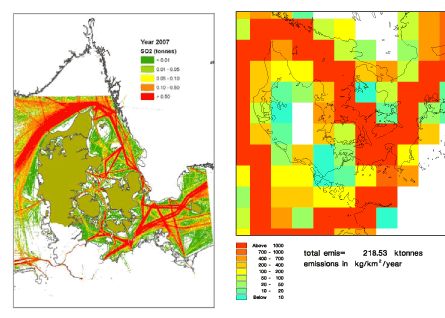
Figur 1 Skibsemissioner af SO2 pr km². Til venstre i henhold til den ny, AIS-baserede emissionsopgørelse med detaljeringsgrad på 1 x 1 km. Til højre i henhold til den tidligere benyttede, hvor emissionen foreligger i felter på 50 x 50 km.
Til sammenligning viser figuren også SO2-emissioner iht. den ældre emissionsopgørelse fra EMEP (2008), der hidtil har dannet grundlag for tilsvarende modelberegninger, og som har en grov opløsning på 50 x 50 km. Den tidligere opgørelse har bl.a. været benyttet ved beregningerne i forbindelse med den danske luftkvalitetsovervågning under NOVANA (Ellermann et al., 2009; Kemp et al., 2008), hvor der dog ikke var specielt fokus på skibstrafik. Den tidligere opgørelse benævnes EMEP-ref (se kapitel 3 og 4). Det fremgår af Figur 1, at den ny AIS-baserede opgørelse i detaljer viser, hvordan skibsruterne fremstår som veldefinerede "veje" til søs, mens de gamle, grovmaskede data indebærer et mere mudret billede, hvor der også forekommer emission fra skibe indenlands, fordi de store gitterfelter dækker både vand og land.
En række andre forskelle er mindre synlige, men betyder noget for emissionerne. I de gamle data blev der regnet med, at skibene sejler med konstant belastning af motoren, mens den ny metode tager hensyn til at der er forskelle i emissionerne, afhængigt af skibets hastighed. Den gamle metode byggede på antagelser om sejlruten mellem havnene, mens AIS-metoden tager udgangspunkt i de faktiske sejlruter, baseret på data fra 24 døgn i 2007.
Den ny metode anses for et væsentligt fremskridt i forhold til den tidligere; dog er der fortsat mulighed for forbedringer – f.eks. udvidelse af området med AIS-signaler og inddragelse af en større mængde AIS-data end de 24 dage, der nu udgør basis for beregningerne.
Forudsætninger for scenarierne
De væsentligste forudsætninger for scenarie-beregningerne er som følger.
- De vedtagne IMO reguleringer for svovl og NOX gennemføres som planlagt. Specielt er det forudsat, at farvandene omkring Danmark udpeges til en såkaldt NOX Emission Control Area (NECA) som defineret af IMO. Østersø-landene forbereder en ansøgning herom. Status som NECA indebærer skærpede krav om NOX-udledninger, specielt for nye skibe efter 2016.
- 2020-scenariet bygger på en forudsætning om uændret skibstrafik frem til 2011 og derefter en stigning på 3,5% pr år for fragtskibe i perioden 2011-2020. Der antages uændret passagertrafik.
- Hvad angår landbaserede emissioner er benyttet et specifikt sæt forudsætninger. Der forventes i nær fremtid fremsat forslag til nyt internationalt direktiv om nationale emissionslofter (NEC-direktivet), som skal være overholdt i 2020. Direktivet er imidlertid ikke fremlagt endnu, så derfor anvendes et scenario for udledninger fra de landbaserede kilder i Europa i 2020, der er sammensat ud fra EU’s temastrategi for ren luft i Europa (se bl.a. Bach et al., 2006) og scenarier for EU-27 udarbejdet af International Institute for Applied Systems Analysis (Amann et al., 2008), som led i det forberedende arbejde i forbindelse med et nyt NEC-direktiv. Detaljer findes i afsnit 4.4.
Emissioner i henhold til scenarierne
Figur 2 viser brændstofforbrug samt emissioner fra skibstrafik for de tre scenarieår 2007, 2011 og 2020 i farvandene omkring Danmark - nærmere bestemt det område, der er farvet i Figur 1 tv.
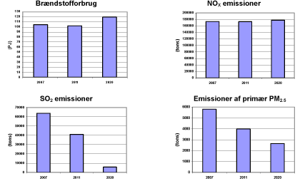
Figur 2 Brændstofforbrug (Petajoule) samt emissioner fra skibstrafik i farvandene omkring Danmark (jvnf. Figur 1) for de tre scenarieår 2007, 2011 og 2020.
Der beregnes en vækst på 15% i brændstofforbruget fra 2007 til 2020, hvilket er et resultat af øget trafikmængde (36% forøgelse for fragtskibe og uændret passagertrafik), kombineret med at motorerne i skibsflåden gradvis bliver mere effektive.
For kvælstofoxider (NOX) forventes en svag stigning i emissionen på 2% fra 2007 til 2020. Uden strengere krav til emissionerne ville stigningen have svaret til forøgelsen i brændstofforbrug (15%). Resultatet af IMO-restriktionerne er altså en gennemsnitlig reduktion i NOX-emissionerne på 11% per kg brændstof. Sådanne reduktioner fortsætter efter 2020.
For svovldioxid (SO2) forudses fra 2007 til 2020 en reduktion på 91%, mens reduktionen for primær PM2.5 er 54%. Primære partikler udgør kun en lille del af den mængde partikler, man finder i luften (se afsnittet Koncentrationer af partikler her i sammenfatningen for forklaring af primære og sekundære partikler).
De mest markante reduktioner i skibsemissionerne sker for SO2. Disse reduktioner illustreres på kortene i Figur 3. Kortene giver et overblik over skibstrafikken omkring Danmark. Meget synlige er hovedskibsruterne fra den Botniske Bugt til Nordsøen, de større indenlandske færgeruter, samt færgeruterne der forbinder Danmark, Sverige, Tyskland og Polen.
Koncentrationer af svovldioxid
Hvad angår forurening med SO2 har skibstrafik hidtil været en meget markant kilde. Fra ca. 2007 har skibe i Østersøen og Nordsøen været underlagt et krav om at svovlindholdet i olien højst må være 1,5%, mens det tidligere typisk var 2,7% (sektion 3.1). Skibstrafik fremstår dog stadig som en væsentlig kilde, sammenlignet med kilder på landjorden. Figur 4 viser beregnede koncentrationer af SO2, dels for en 2007-situation (med 1,5% svovl), dels for situationen i 2020. I 2020 vil svovlkravet være betydeligt skærpet, nemlig til 0,1%, og det afspejler sig tydeligt i koncentrationen i luften.
Siden 1990 er der sket en væsentlig reduktion af SO2-emission fra landbaserede kilder, og reduktionen forventes at fortsætte. Resultatet vil i 2020 være, at SO2-koncentrationen som middelværdi i Danmark vil være nede på blot 0,3 μg/m³, hvilket er 6% af 1990-niveauet.
Figur 5 viser det relative bidrag fra skibstrafik - i forhold til samtlige kilder - til koncentrationsniveauet af SO2 samt flere andre forureningskomponenter. Der er tale om et gennemsnit over hele Danmark. Figuren viser resultater fra to sæt beregninger: Dels beregninger på grundlag af den nye, mere præcise emissionsopgørelse (betegnet AIS-2007), dels på grundlag af den ældre opgørelse fra EMEP (betegnet EMEP-ref).
Den ny opgørelse adskiller sig fra den gamle på flere måder: den forudsætter at svovlprocenten i brændslet er 1,5%, mens den gamle refererede til situationen før 2007 og benyttede 2,7%; den ny har højere geografisk opløsning; den er baseret på mere korrekte skibsruter end den gamle; og den bruger mere realistiske data for skibenes motorbelastning. Alle disse faktorer tilsammen betyder, at den ny opgørelse fører til lavere emissioner. Reduktionen er mest markant for svovldioxid og primær PM2.5, men gør sig også gældende for de andre forureningskomponenter. Hvor det på grundlag af den ældre emissionsopgørelse fra EMEP blev vurderet at skibe stod for 68% af SO2-niveauet i Danmark, er andelen nede på 37% i henhold til den ny opgørelse.
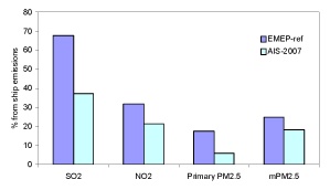
Figur 5 Relativt bidrag fra skibe til koncentrationsniveauet i luften af forskellige forurenende stoffer. Farven på søjlerne viser, hvilken emissionsopgørelse der ligger til grund for de beregnede koncentrationer. De lyseblå søjler betjener sig af den nye, mere præcise opgørelse ("AIS-2007"). De mørkeblå af den ældre emissionsopgørelse fra EMEP ("EMEP-ref").
Koncentrationer af NO2
Det er ved beregningerne forudsat, at farvandene omkring Danmark udpeges til et såkaldt NOX Emission Control Area, som defineret af IMO, hvor der gælder skærpede NOX-krav. Det mest markante krav gælder nye skibe fra 2016, hvor der kræves 80% reduktion af NOX-udledningen. Der er andre, mindre vidtgående krav til ældre skibe.
Resultatet af beregningerne er, at IMO-kravene ikke formår at opveje den forudsete stigning i skibstrafikken. I år 2020 forudses stort set samme niveau af NOX-emissioner fra skibsfart som i 2007-situationen. Efter 2020 vil IMO-kravene formentlig ytre sig i lavere skibsemissioner, men det er ikke tilfældet i 2020. Derimod sker der markante ændringer på land i henhold til det ovennævnte scenario for emissionerne i 2020.
Resultatet ses i Figur 6. NOX leder til dannelse af NO2, som der gælder sundhedsrelaterede grænseværdier for. Figur 6 viser beregnede koncentrationer af NO2, dels for en 2007-situation, dels for situationen i 2020. De store skibsruter forbliver særdeles synlige, mens koncentrationen på landjorden aftager. Andelen af skibes bidrag til NO2-koncentrationsniveauet er i 2007 21%, mens den vil stige til 34% i 2020 - fordi de øvrige kilders emission reduceres.
Det er et meget interessant resultat af beregningerne, at bybaggrundsniveauet af NO2 i København forventes at falde med ca. 7 μg/m³ i tiden fra 2007 til 2020. NO2-niveauerne på mange københavnske gadestrækninger overstiger EU's grænseværdi på 40 μg/m³, og i lyset heraf er et så stort fald i baggrundsniveauet interessant.
Koncentrationer af partikler
Fine partikler med en diameter på mindre end 2,5 mikrometer betegnes som PM2.5. Man kan yderligere sondre mellem forskellige typer partikler, der indgår i PM2.5. Primære partikler forefindes som partikler umiddelbart efter at de har forladt kilden. Sekundære partikler er derimod partikler, der ikke er "født" som partikler, men er dannet ved omdannelse af gasarter - typisk mange timer efter at forureningen er sendt ud i atmosfæren. De sekundære partikler kan yderligere underopdeles i sekundære uorganiske og sekundære organiske.
Skibes udledning af SO2 og NOX giver anledning til dannelse af sekundære uorganiske partikler, og hele denne mekanisme indgår i den benyttede luftforureningsmodel, DEHM. Hvad angår de sekundære organiske partikler har man ikke tilstrækkelig viden til at kunne beskrive dem modelmæssigt. Dette gælder også på internationalt niveau (se bl.a. Yttri et al., 2009). Derfor beskriver modellen kun en delaf den mængde partikler, man finder i atmosfæren, nemlig primære og sekundære uorganiske partikler. I rapporten omtales denne del som mPM2.5.
Figur 7 viser beregnede koncentrationer af mPM2.5. PM2.5 kan transporteres over store afstande, mens SO2 og NO2 ikke har lige så lang levetid. Derfor adskiller det geografiske mønster i Figur 7 sig markant fra mønstret i de foregående figurer. Skibenes forurening er ikke synlig, mens det er markant, at forurening fra det centrale Europa gradvis klinger af hen over Danmark. Skibstrafikkens bidrag til mPM2.5 er 18%, mens bidraget set i forhold til atmosfærens totale PM2.5-niveau er en del mindre. Det vurderes at i forhold til total PM2.5 i København er skibstrafiks bidrag omkring 4-7%, afhængigt af om man betragter luften i en trafikeret gade eller i by-baggrund (dvs. væk fra selve gaden).
Frem til 2020 vil der ske en reduktion af det generelle niveau af mPM2.5 over Danmark på lidt over 2 μg/m³, hvilket hovedsagelig skyldes reduktion i landbaserede emissioner.
Summary and conclusions
Background and objectives
Ship traffic in the Danish marine waters is considered to be important for air quality in Danish cities and in Denmark in general. Previously, the Danish National Environmental Research Institute at Aarhus University (NERI, in Danish Danmarks Miljøundersøgelser) has provided certain estimates for the significance of shipping to air pollution (e.g. Olesen et al., 2008). However, these previous estimates were subject to a high degree of uncertainty. They were based on emission inventories with a low geographical resolution (50 km x 50 km). Furthermore, they were based on simplifying assumptions, which do not necessarily reflect the actual patterns of ship traffic.
However, since 2006 the so-called Automatic Identification System (AIS) has registered ship activities in Danish marine waters. All ships larger than 300 GT (Gross Tonnage) are required to carry a transponder, which transmits information on the ship’s identity and position to land-based receiving stations. This information makes it possible to map ship emissions in much greater detail than previously feasible. This opportunity has now been utilised to create a new emission inventory for ships in the Danish marine waters.
The new AIS-based inventory of ship emissions has been combined with other necessary data and used as basis for new model calculations of air quality in Denmark. A main objective of this work is to assess the contribution from ships to concentration levels of various pollutants. For the modelling of concentrations, a new version of the air pollution model DEHM (Danish Eulerian Hemispheric Model) has been applied - a version with a higher geographical resolution than the previous version.
The International Maritime Organisation (IMO) has adopted new regulations in order to reduce pollution from ships with sulphur dioxide (SO2) and nitrogen oxides (NOX) in the period until 2020. It is also the objective of this work to investigate the effect of this regulation on air quality in Denmark. This is done through scenario calculations for air quality for 2020 based on expected emission reductions.
Also for land-based sources of SO2, NOx and particles, emission reductions are envisaged before 2020. The scenario calculation for 2020 takes account of these reductions.
A minor component of the current study concerns the contribution from ships at port to local air pollution in the ports of Copenhagen and Aarhus.
The study
The study has been carried out by NERI at Aarhus University. As one of the main parts of the study a new, improved inventory of ship emissions in the Danish marine waters has been established. Both new (NERI) and old (EMEP, 2008) emission inventories have been applied for model calculations of air quality in Denmark, thus allowing an assessment of the effect of the revised inventory.
Furthermore, scenario calculations for 2011 and 2020 have been carried out, in order to evaluate the effect of the IMO regulations. The scenario calculations have been based on expected reductions in ship emissions and an estimate for land-based emissions in 2020.
Finally, the contribution to local air pollution from ships at ports has been assessed in various ways, based on updates of previous studies.
Main conclusions
Concerning emissions:
- One of the main results of the project is that a new, improved emission inventory for national and international ship emissions in Danish marine waters has been established. The inventory has a spatial resolution of 1 x 1 km. Previous inventories from the European Monitoring programme EMEP applied a grid size of 50 x 50 km. A comparison between the measured concentrations and model results based on the old (EMEP) inventory and the new (NERI) inventory shows that the new inventory is a considerable improvement.
- Between 2007 and 2020 an emission reduction as large as 91% is envisaged in the marine waters around Denmark, in respect to sulphur dioxide from ship traffic - despite an increase of traffic. This is due to the IMO regulations.
- Within the same period a marginal increase is expected in total emissions of nitrogen oxides (NOX) from ship traffic, namely by 2% from 2007 to 2020. Without stricter emission standards the increase would have corresponded to the increase in fuel consumption, i.e. 15%. The IMO requirements imply large NOX reductions for new ships from 2016. As a consequence, the ship fleet will gradually experience a reduction in its average NOX emission factor from 2016 onwards; this development will continue after 2020.
Concerning concentrations:
- Since 1990, SO2 emissions from land-based sources have been substantially reduced, and in the years to come a continued large reduction from ship traffic is expected, along with an expected reduction for land-based sources. Based on scenario calculations the SO2 concentration level as an average for Denmark will decrease considerably in the period up to 2020, so in 2020 it will reach a level of 0.3 μg/m³, which is only 6% of what it was in 1990, and corresponds to 1.5% of the EU limit values. In 2007 around 33% of the SO2 concentration level in Denmark was due to ship emissions, this number will be reduced to about 11% in 2020.
- The concentration of nitrogen dioxide (NO2) in urban background air in Copenhagen is expected to be reduced from 16 to 9 μg/m³ in the period up to 2020. The reduction is due to expected reductions in NOX emissions from land-based sources. For ship traffic, however, the contribution is essentially unchanged, because increase in ship traffic and stricter emission requirements balance each other. For Denmark as a whole the NO2 concentration level is considerably lower than in Copenhagen, and it will decrease from 5.5 to around 3.5 μg/m³ from 2007 up to 2020. Presently, as an average for Denmark, 21% of NO2 can be attributed to ship traffic, but the relative share from ships will increase in the years up to 2020 due to reductions for the land-based sources.
- A considerable amount of fine particles (PM2.5) is of unknown origin. Internationally, this is recognised as being state-of-the-art. The fraction that can be explained and modelled is here designated mPM2.5 (modelled PM2.5, see the section Concentrations of particles here in the summary for further explanation). Around 1 μg/m³ of the mPM2.5 level can be attributed to ships, both in Copenhagen and generally in Denmark. Calculations point to a slight decrease by approximately 0.2 μg/m³ during the period to 2020. If one wishes to express the ship contribution in terms of percent, the fraction attributable to ships will depend on the location considered, as well as whether the mPM2.5 contribution is compared to the value for mPM2.5 or for total PM2.5. Compared to total PM2.5, the percent wise contribution in urban background air in Copenhagen will be on the order of 7%.
- A comparison between concentration results based on the previous (EMEP) and the new (NERI) inventories show that the new inventory results in concentrations that are lower by, respectively, 46% for SO2, 14% for NO2 and 10% for mPM2.5 (average concentrations over Denmark).
- According to the new inventory the amount of ship traffic through the Øresund is larger than according to the previous (EMEP). As a consequence, emissions in the Øresund are larger than previously assessed. On the other hand, in the Storebælt and Kattegat ship emissions are substantially smaller than previously estimated. In the case of sulphur dioxide, the emission in Storebælt was previously assessed to be 11 times larger than that of Øresund; now, the emission in Storebælt is assessed to be only 2.3 times larger. Altogether, the emissions around Zealand are smaller than previously assessed, and the resulting level of sulphur dioxide in ambient air is smaller than previously assessed. For the Copenhagen region the average SO2 concentration is estimated at 1 μg/m³, to be contrasted with the previous estimate of 1.6 μg/m³.
Concerning ships at port:
- In the port of Copenhagen cruise ships are responsible for 55% of the total NOX emission from ships at port. Anyhow, this does not lead to problems related to NO2 limit values around the docks, and neither does it create problems with respect to limit values for PM2.5 and SO2.
- When considering conditions at high rise buildings close to berths with very heavy ship traffic, there may potentially be problems with NO2 exceedances very close to the berth (within the nearest hundred or few hundred meters). In such cases it can be wise to conduct detailed studies.
- Section 5.10 of the report indicates some further conclusions concerning local air pollution from ships at port.
Project results
The AIS-based emission inventory
The project has resulted in a new, AIS-based emission inventory for ship traffic in the Danish marine waters. It is based on detailed information, both in respect to geographical resolution, and to the underlying information on the pollution from the individual ships. As an example Fig. 1 shows the detailed emission inventory for SO2 with a resolution of 1 x 1 km. For the modelling purposes, however, a spatial resolution of 6 x 6 km is used, corresponding to the resolution of the air pollution model.
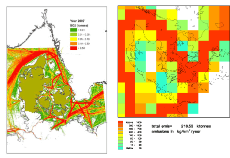
Fig. 1 Ship emissions of SO2 pr km2. The left panel displays values from the new, AIS-based emission inventory with a resolution of 1 x 1 km. The right panel illustrates the previously used inventory, where the emission is assigned to grid cells of size 50 x 50 km (EMEP, 2008).
For comparison, Fig. 1 also shows SO2 emissions according to the previous inventory from EMEP (2008), which has been the base for model calculations until now, and which has a crude resolution of 50 x 50 km. The previous inventory has been used for calculations in the framework of the Danish monitoring programme NOVANA (Ellermann et al., 2009; Kemp et al., 2008) - which, however, did not have particular focus on ship traffic. The previous inventory is referred to as EMEP-ref (se Chapters 3 and 4).
It appears from Fig. 1 that the new AIS-based inventory in detail shows how the ship routes appear as well-defined 'roads' at sea, as opposed to the old method, which has grid cells extending over both sea and land, and thus places some emissions from ships over land.
Other differences are less visible, but have consequences for the emissions: The previous inventory assumed that the engine load for ships was constant, whereas the new method takes account of differences in emissions, depending on the speed of the ship. The old method applied assumptions concerning the ship routes, whereas the AIS method is based on actual routes, based on a sample of 24 days in 2007.
The new method is regarded as a considerable improvement compared to the previous; however, there is still room for improvement – e.g., extension of the area with AIS signals, and use of a larger amount of AIS data than the 24 days which form the basis for the present calculations.
Assumptions for scenarios
The main assumptions underlying the scenario calculations are as follows.
- The IMO regulations for sulphur and NOX are implemented as planned. In particular, it is assumed that the marine waters around Denmark will be designated a NOX Emission Control Area (NECA) as defined by IMO. The countries around the Baltic Sea are preparing an application with this purpose. The status as NECA implies additional NOX emission restrictions for new ships from 2016.
- Concerning the amount of ship traffic, an annual increase of 3.5 percent has been assumed for transport of goods from 2011 and onwards, while passenger traffic is assumed unchanged.
- Concerning land-based emissions, a specific set of assumptions have been used. It is expected that in near future a new EU directive on national emission ceilings for 2020 (NEC directive) will be negotiated. However, there is not yet an official proposal for the directive. Therefore a scenario for emissions from land-based sources in Europe in 2020 has been set up, which is based on emission scenarios prepared in connection with EU's thematic strategy for clean air in Europe (see e.g. Bach et al., 2006), and scenarios for EU-27, prepared by the International Institute for Applied Systems Analysis (Amann et al., 2008) as part of the preparatory work for a new NEC directive. Further details are found in Section 4.4.
Emissions according to the scenarios
Fig. 2 displays the fuel consumption and emissions from ship traffic for the three scenarios: 2007, 2011 and 2020. The values refer to the area which is colored in Fig. 1(left).
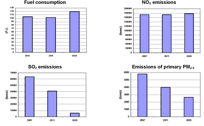
Fig. 2 Fuel consumption (Petajoule) and emissions from ship traffic in the waters around Denmark (cf. Fig. 1) for the three scenario years 2007, 2011 and 2020.
The calculations predict a 15% increase in fuel consumption from 2007 to 2020 as a result of increased traffic (36% increase for freight ships and unchanged passenger traffic), combined with increased efficiency for ship engines.
For emissions of nitrogen oxides (NOX) there is an expected growth of 2% between 2007 and 2020. Without stricter emission requirements the increase would have corresponded to the increase in fuel consumption (15%). Accordingly, the result of the IMO reductions is an average reduction in NOX emisssions of 11% per kg of fuel. Such relative reductions are expected to continue after 2020.
For sulphur dioxide (SO2) a reduction of 91% is envisaged between 2007 and 2020, while for primary PM2.5 the reduction is 54%. Primary particles account for only a minor fraction of the total amount of particles found in ambient air (see the section Concentrations of particles in this summary).
The most pronounced reductions in ship emissions take place for SO2. These reductions are illustrated in Fig. 3. The maps yield an overview of sea traffic around Denmark. Clearly visible are the main shipping lanes from the inner Baltic Sea (Bothnian Bay) to the North Sea, the major Danish domestic ferry routes, and the ferry routes connecting Denmark, Sweden, Germany and Poland.
Concentrations of sulphur dioxide
Ship emissions are a major source to pollution with SO2. Since 2007 it has been a requirement for ships in the Baltic Sea and the North Sea that the sulphur content in fuel should not exceed 1.5%, whereas previously it typically was 2.7% (Section 3.1). Nevertheless, ships are still an important source in comparison with land-based sources. Fig. 4 shows calculated concentrations of SO2, referring to, respectively, 2007 (with 1.5% sulphur in fuel) and 2020. The requirement to sulphur content in 2020 is considerably more restrictive than now (max. 0.1% sulphur), and this is clearly reflected in computed concentrations for 2020.
Since 1990, SO2 emissions from land-based sources have been substantially reduced, and in the years to come the reduction is expected to continue. Scenario calculations show that the SO2 concentration level for Denmark will decrease considerably over the period up to 2020, so in 2020 it will reach a level of 0.3 μg/m³, which is only 6% of what it was in 1990.
Fig. 5 shows the relative contribution from ship traffic, compared to the total from all sources, for SO2 as well as for several other pollutants. The values refer to an average over Denmark. The figure shows results from two sets of calculations: Calculations based on the new, more precise emission inventory (denoted AIS-2007), and calculations based on the older inventory from EMEP (denoted EMEP-ref).
The new inventory differs from the old in several respects: it assumes that sulphur content in fuel is 1.5 %, while the old refers to the situation before 2007 and uses 2.7 %; the new has a higher geographical resolution; it is based on more correct ship routes than the old; it uses more realistic data for the load of ship engines. The combined effect of all of these factors is that the new inventory has lower emissions. The reduction is most pronounced for SO2 and primary PM2.5, but also applies to other compounds. Whereas the calculations based on the previous inventory from EMEP ascribed 68% of the SO2 concentration level in Denmark to ship emissions, calculations based on the new inventory ascribe only 37% to ships.

Fig. 5 Relative contribution from ships to the average concentrations of various pollutants in Denmark. The colour indicates which emission inventory the calculations are based on. The light blue columns use the new, more precise inventory ("AIS-2007"). The dark blue use the old emission inventory from EMEP ("EMEP-ref").
Concentrations of nitrogen dioxide (NO2)
IMO has adopted regulations of NOX emissions. In the present study it is assumed that the marine waters around Denmark will become designated a so-called NOX Emission Control Area as defined by IMO. This implies several restrictions on NOX emissions, in particular for new ships from 2016, where an 80 percent reduction in NOX emission is required. There are other, less demanding requirements to older ships.
However, at the same time an increase in ship traffic is foreseen. The reduction in emissions is not able to completely outbalance the foreseen increase in ship traffic, so the NOX emission from ships will be slightly higher in 2020 than in 2007. It is likely that the IMO requirements will result in lower ship emissions after 2020, but this is not the case for 2020. On the other hand, there are marked changes for land-based sources according to the scenario for 2020.
The result in terms of concentrations is seen in Fig. 6. NOX leads to formation of NO2, for which health-related limit values exist. Fig. 6 shows model calculated concentrations of NO2 for 2007 and 2020, respectively. respectively. The large shipping routes remain clearly visible, but inland concentrations decrease. The share from ships to the NO2 concentration level is 21% in 2007, but increases to 34 % in 2020 - because the absolute contribution from other sources is reduced.
It is an interesting result of the calculations that the concentration of NO2 in urban background in Copenhagen is expected to be reduced by 7 μg/m³ (from 16 to 9 μg/m³) in the period up to 2020. In several highly trafficked streets in Copenhagen the EU limit value of 40 μg/m³ is exceeded; this fact makes a large drop in background levels very interesting.
Concentrations of particles
Fine particles with a diameter less than 2.5 micrometer are referred to as PM2.5. One can distinguish between primary particles and secondary particles. Primary particles exist as particles immediately after they have left the source. Secondary particles were not 'born' as particles, but are created from gases, which undergo chemical transformation during transport – a process that continues for several hours or days after the pollution has left the source. Secondary particles can be further characterised as secondary inorganic particles or as secondary organic particles.
Emissions of SO2 and NOX from ships contribute to the formation of secondary inorganic particles. The DEHM model which is used for calculations of concentrations takes account of the processes involved. However, there is insufficient knowledge to describe the formation of secondary organic particles, and DEHM does not account for these. Internationally, this is recognised as being state-of-the-art for current models (see Yttri et al., 2009). Accordingly, the DEHM model accounts only for a certain fraction of the particles found in the atmosphere, namely the primary and the secondary inorganic. This part is here designated mPM2.5 (modelled PM2.5).
Fig. 7 shows calculated concentration levels of mPM2.5. PM2.5 can be transported over large distances, whereas SO2 and NO2 have a shorter atmospheric lifetime. This is the reason why the geographical pattern in Fig. 7 is very dissimilar to the previous figures. The pollution from ships is not visible, while it is a dominant feature that pollution from central Europe gradually declines over Denmark. The share of mPM2.5 attributable to ship traffic is 18%, while in terms of total PM2.5 the share from ships is considerably smaller. Relative to total PM2.5 in Copenhagen, the share from ship traffic can be estimated to around 4-7%, depending on whether one considers the air in a highly trafficked street or in urban background (e.g. a park).
In the time up to 2020 a reduction of the general level of mPM2.5 will take place, amounting to slightly more than 2 μg/m³. This is mainly due to emission reductions for land-based sources.
1 Introduction
- 1.1 Background
- 1.2 AIS data
- 1.3 New regulations and projections
- 1.4 Relation to previous studies
- 1.5 Structure of the report
The work described in the present report covers several aspects of the contribution from ships to air pollution in Denmark. The main focus of the report is to describe a newly developed and more accurate emission inventory for air pollution related to ship traffic in the Danish marine waters, and to use this inventory to determine the contribution from ships to concentration levels within Denmark. Further, the study includes scenario calculations for years 2011 and 2020. These scenario calculations are used to assess the effect that international regulations of ship emissions and other regulations will have for the future air pollution in Denmark. A minor component of the work concerns the contribution from ships at port to local air pollution in the ports of Copenhagen and Aarhus.
1.1 Background
Emissions from ship engines contribute to air pollution with sulphur dioxide (SO2), nitrogen oxides (NOX), particulate matter (PM) and Volatile Organic Compounds (VOC). Furthermore, ship engines emit the greenhouse gas CO2. Focus of the present report is, however, on traditional pollutants, not on CO2.
Previous investigations have made clear that the contribution from ships to emission of SO2 and NOX is considerable, compared to land-based sources, and that there is a substantial effect on inland concentrations. It is important to note that even though NOX and SO2 are gases, they will contribute to the formation of particles. Some of the particles present in ambient air have been emitted as particles (primary particles), while others (secondary particles) have been formed through chemical and physical reactions in the atmosphere. Thus, although SO2 and NOX are emitted as gases, they will affect inland concentration levels for both these gases themselves, as well as for reaction products, including particles.
Pollution with particles is of considerable interest, because particles are associated with negative health effects. A commonly used measure for particle pollution is concentration in terms of PM2.5, i.e. particles smaller than 2.5 micrometer. This is referred to as the fine fraction of particle pollution.
As mentioned above, one can distinguish between primary particles and secondary particles. Secondary particles can be further characterised as secondary inorganic particles or as secondary organic particles. All types of particles are present in ambient air. Note, however, that emission inventories take account only of primary particles, because only these are actually emitted from the sources. The DEHM model - which is applied to compute concentration levels in ambient air in Chapter 4 - also takes account of the formation of secondary inorganic particles. Some of these originate from ship emissions of SO2 and NOX. However, DEHM does not account for secondary organic particles. This question is elaborated in Chapter 4, in particular sections 4.2 and 4.9.
The present study represents no attempt at evaluation of health effects; it considers only concentration levels of various compounds.
1.2 AIS data
Since 2006 the so-called AIS system - Automatic Identification System - has been implemented in the marine waters around Denmark. It is required that all ships greater than 300 GT carry an AIS transponder. With very short time intervals the transponder transfers signals to land-based stations, providing information on ship identity, position, destination etc. This type of information provides the basis for estimates of the ship emissions and their spatial distribution in the present study. The methodology is described in detail in Chapter 2. The spatial distribution of emissions becomes much more precise with use of AIS data than with previously available data.
In the present study, AIS data were requested from DaMSA (Danish Maritime Safety Administration). Since AIS signals represent a huge amount of data, only data from a limited area around Denmark were requested from DaMSA as illustrated in Figure 1.1. Furthermore, in order to represent the year 2007, not all data for the entire year was considered. The present project uses 12 two-days periods, one period for each month, representing both weekend days and normal working days. From DaMSA data the following information was used: Vessel IMO and MMSI codes, call sign, time of AIS signal, and latitude-longitude coordinates. For each ship, the sailing speed between two AIS signals was calculated from the time between the signals, and the corresponding latitude-longitude registrations.
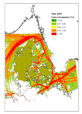
Figure 1.1 Fuel consumption according to AIS data with application of the methodology described in chapter 2. The unit is TJ/km². The coloured area on the map illustrates where the AIS data are applied in the present study. In the following, it will be referred to as the AIS inventory area.
79 % of the ships were identified as entries in Lloyd’s Registers technical database. A reasonable assumption was that the ships not included in the latter database were merely small vessels. Further assessment of the number of ships and fuel consumption estimates, also made it reasonable to assume that emission results the 12 periods could be extrapolated to cover a full year emission estimate.
1.3 New regulations and projections
The present study considers the current situation, as well as two projections. In 2008, the International Maritime Organisation (IMO) agreed on new, stricter rules for the emissions of SO2 and NOX, to be implemented stepwise in the period towards 2020.
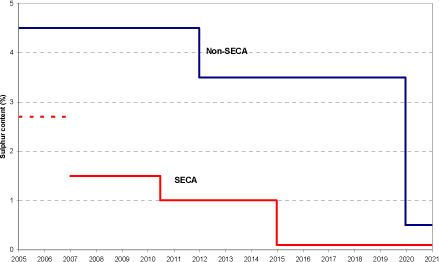
Figure 1.2 Limit to sulphur content in heavy fuel oil, according to IMO regulations. The SECA regulations were implemented in the Baltic Sea in 2006 and in the North Sea in August 2007. For calculations in the present report, SECA regulations have been assumed in effect during the entire year of 2007. The broken line indicates 2.7% which was the assumed level prior to 2007.
Figure 1.2 illustrates the requirements for sulphur content in heavy fuel oil, which is the most common marine fuel. SECA stands for SOx Emission Control Area. The curve labelled Non-SECA represents the general requirements, applicable everywhere. In SECA's requirements are stricter. The Baltic Sea and the North Sea[¹] have been appointed SECA areas, with the stricter requirements implemented in 2006 and August 2007, respectively (see chapter 2 for details). Prior to 2006, the sulphur content in fuel used by ships in these areas has assumed to be 2.7%, in accordance with Cofala et al. (2007) - see Section 3.1 for more details.
The basic scenario that is taken to represent the current situation is the year 2007. In computations for this scenario it has been assumed that the Baltic Sea and North Sea were SECA areas during all of 2007.
NOx emissions are regulated by IMO (Marpol 73/78 Annex VI, and further, amendments) in a three tiered emission regulation approach, as follows:
- Tier I: Diesel engines (> 130 kW) installed on a ship constructed on or after 1 January 2000 and prior to 1 January 2011.
- Tier II: Diesel engines (> 130 kW) installed on a ship constructed on or after 1 January 2011.
- Tier III: Diesel engines (> 130 kW) installed on a ship constructed on or after 1 January 2016.
Tier III applies only in areas, which have been designated NOX Emission Control Area (NECA). The countries around the Baltic Sea are preparing an application to obtain this status for the Baltic Sea. It is assumed for the 2020 scenario that the marine waters around Denmark are a NECA.
As it appears from Figure 1.2 there will be substantial reductions in sulphur content in SECA areas in 2010 and 2015. Furthermore, the NOx emissions from new engines become significantly lower in the period considered. The effect of these measures has been studied, based on projected emission scenarios for the years 2011 and 2020, in addition to the baseline scenario for 2007.
The scenarios take account of a general increase in ship traffic during the period up to 2020. In accordance with expectations from the Danish Ship-owners' Association (see chapter 2) it has been assumed that, due to the financial crisis, ship traffic has dropped since 2007, but will again in 2011 reach the level of 2007. From 2011 and onwards, an annual increase of 3.5 percent has been assumed for transport of goods, while passenger traffic is assumed unchanged.
1.4 Relation to previous studies
Many previous studies from NERI have included emissions from ships as one of the sources to air pollution, whereas they have not addressed the contribution from ships separately. Among such studies are annual reports on the Danish monitoring programmes (e.g. Kemp et al., 2008; Ellermann et al., 2009).
The present study is the first to make use of AIS data for air pollution studies in a Danish context. In other countries the use of AIS data for construction of emission inventories has recently started.
A related study is the report by Winther (2008) on fuel consumption and emissions from navigation in Denmark, which is, however, focussed on national Danish ship traffic.
In 2001, emission inventories for 1995/1996 and 1999/2000 were compiled by Wismann (2001), estimating the fuel consumption and emissions for all sea transport in Danish waters.
Other Danish projects were the assessment of the fuel consumption and emissions for ships in Danish ports (hotelling, manoeuvring, landing/loading) by Oxbøl and Wismann (2003), and the examination of air quality effects from cruise ship activities in the Port of Copenhagen by Olesen and Berkowicz (2005). Other studies concerning pollution in ports are also relevant and will be discussed in Chapter 5.
1.5 Structure of the report
The report has the following structure.
Chapter 2 provides a comprehensive description of the methodology applied for constructing the detailed AIS-based emission inventories, which form the basis for the further calculations. The inventories are for the years 2007, 2011 and 2020. It is described how AIS data obtained from DaMSA are processed in order to determine time, position and speed for each ship in the AIS inventory area. Further, the chapter explains how speed based engine load functions are used to estimate the instantaneous ship engine load. The emission factors are described, as well as relevant ship technical data obtained from e.g. Lloyd’s Register. The emissions are calculated as a product of emission factors, engine size, engine load and time between AIS signals. Emission results are shown for 2007, 2011 and 2020 in details per engine type, fuel type and ship category. Results are also listed per flag state, and GIS maps show the geographical distribution of emissions in the AIS inventory area.
Chapter 3 goes one step further from the AIS-based inventories. In order to apply these inventories in an air pollution model, it is necessary to combine them with emission data covering a much larger geographical data. Chapter 3 presents the inventories for ship emissions that are used for model runs with the air pollution model DEHM (Danish Eulerian Hemispheric Model). It is described how the AIS-based inventories from Chapter 2 are combined with emission data provided by EMEP (Co-operative Programme for Monitoring and Evaluation of the Long-Range Transmission of Air Pollutants in Europe). The EMEP estimates are characterised by a cruder geographical resolution, and there are interesting differences between the two sets of inventories which are discussed.
Chapter 4 describes how the ship emissions are combined with emissions from land-based sources and aviation. However, the bulk of the chapter is devoted to a presentation and discussion of results for concentrations, obtained with the air pollution model DEHM (Danish Eulerian Hemispheric Model). The chapter includes a quantification of the contribution from ships to concentration levels in Denmark. Further, it presents scenario calculations, demonstrating the combined effect on concentration levels of the IMO measures and the expected changes in land-based emissions. Finally, it considers the influence of ship traffic on general concentration levels in the Copenhagen area.
Chapter 5 presents results of studies of local pollution from ships at port in Copenhagen and Aarhus.
Conclusions are found in the section Summary and conclusions in front of the report.
[1] In the context of SECA's the Baltic Sea and the North Sea are larger than their normal delimitation; the two SECA's are adjacent and include the inner Danish waters.
2 Emissions
- 2.1 Introduction
- 2.2 AIS data provided by DaMSA
- 2.3 Vessel data provided by Lloyds
- 2.4 Engine types, fuel types and average engine life times
- 2.5 Traffic forecast
- 2.6 Engine load functions
- 2.7 Fuel consumption and emission factors
- 2.8 Calculation procedure
- 2.9 Results for fuel consumption and emission
- 2.10 Results: Spatial distribution
2.1 Introduction
This chapter provides a comprehensive description of the methodology applied for constructing the detailed AIS-based emission inventories of ship emissions, which form the basis for the further calculations. The inventories are for the years 2007, 2011 and 2020. Furthermore, the chapter summarises results.
After a brief overview of the entire approach, the subsequent sections provide details.
For the 'AIS inventory area' defined in Figure 1.1, AIS data have been requested from the Danish Maritime Safety Administration (DaMSA; in Danish: Farvandsvæsenet). In order to calculate fuel consumption and emissions for ships in the area, these data are used together with vessel technical information from Lloyd’s Register, engine load functions provided by DTU (Technical University of Denmark), and general fuel consumption and emission factors provided by NERI. In order to facilitate the inventory calculations, assumptions are also made regarding fuel type used, engine types and average engine life times.
For each single vessel in the AIS dataset, ship category, engine type, fuel type, main engine and auxiliary engine size are determined using the technical data from Lloyds Register and supplementary information from DTU and MAN Diesel. The vessel sailing speed is found between each AIS signal, and the instantaneous engine load is calculated from basis functions (representing five common ship classes), using main engine size and vessel sailing speed as input.
The fuel consumption and emissions from each vessel during the time between two consecutive AIS signals are calculated by combining engine size, engine load, time duration between the AIS signals, and fuel consumption/emission factors corresponding to the vessel’s engine and fuel type. The baseline results are calculated for the year 2007, and results for the prognosis years 2011 and 2020 are obtained by using forecasted fuel consumption/emission factors from NERI and expectations for sea traffic growth from Danish Ship-owners' Association.
2.2 AIS data provided by DaMSA
AIS signals represent a huge amount of data. In order to restrict the volume of data, a limited area around Denmark (Figure 1.1) was appointed as being of primary interest, and only data from that area were requested from DaMSA. Furthermore, in order to represent the year 2007, not all data for the entire year was considered. The present project uses 12 two-days periods, one period for each month, representing both weekend days and normal working days. The following AIS data are used: Vessel IMO and MMSI codes, call sign, time of AIS signal, and latitude-longitude coordinates. For each ship, the sailing speed between two AIS signals is calculated from the time between the signals, and the corresponding latitude-longitude registrations.
Table 2.1 shows the selected date and day combinations for the different months in 2007, and the corresponding percentage of AIS signals (from the DaMSA dataset) pertaining to identified ships, and the number of ships that could be identified as entries in Lloyd’s Register’s technical database. The total number of AIS signals in DaMSA data is 15.725 mio. (not shown), and the total percentage of identification is 79 %. Based on information from Lloyd's (pers. comm., A. Halai, Lloyds Register, 2009) the unidentified ships are assumed to be merely small sized vessels. Thus, it is well known that many modern pleasure craft have AIS systems installed. Consequently, the bias introduced in the subsequent fuel consumption and emission calculations is regarded as marginal.
Click here to see: Table 2.1 Days selected for AIS data capture.
Figure 2.1 displays the number of ships for each month’s 48-hour period. The number of ships varies to some extent from period to period; however, the range of variation is limited. The same conclusion can be drawn from the corresponding fuel consumption results shown in Figure 2.7 in section 2.9. Based on these observations it is considered a reasonable assumption that the total number of signals obtained from DaMSA for the time periods in question can be extrapolated to cover a full year by using a multiplication factor of 365/24, and that this will result in a reasonably reliable estimate of fuel consumption and emissions from the subsequent inventory calculations.
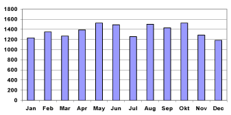
Figure 2.1 Number of ships for each month’s 48-hour period in DaMSA data, identified as entries in the Lloyd’s Register’s technical database.
2.3 Vessel data provided by Lloyds
Relevant technical data for each ship is found by linking the vessel's IMO and MMSI codes and call sign from AIS data to the technical registrations from Lloyd’s Register’s database. The latter data consists of main engine size, engine stroke type (2-stroke/4-stroke), vessel flag and general ship category. The information on general ship category is used to group the vessels into five ship classes (representative types) for which engine load functions can be established (c.f. section 2.6). The Lloyd’s ship categories and the representative ship classes are shown in Annex A.
2.4 Engine types, fuel types and average engine life times
From Lloyds' database a distinction between 2-stroke and 4-stroke engines as well as gas turbine engines is given. It is necessary to further allocate these data into the general engine types: Gas turbine, slow speed, medium speed and high speed engines for which fuel consumption and emission data are available. The following table shows the applied classification, which is based on information from MAN Diesel (pers. comm., Flemming Bak, 2009) and Winther (2008).
Table 2.2 Estimated main engine type and fuel type for ship engines in the present inventory
| Engine type | Engine size | Engine type | Fuel type | Engine life time |
| (Lloyd’s Register) | (kW) | (estimated) | (estimated) | (years, estimated) |
| Gas turbine | Gas turbine | Diesel | 30 | |
| 2-stroke | Slow speed (2-stroke) | HFO | 30 | |
| 4-stroke | <= 1000 | High speed (4-stroke) | Diesel | 10 |
| 1000-4000 | Medium speed (4-stroke) | Diesel | 30 | |
| > 4000 | Medium speed (4-stroke) | HFO | 30 |
2.5 Traffic forecast
The Danish Ship-owners' Association was requested to provide a forecast for the development in ship traffic for the present study. The Association expects that in 2011 the amount of traffic will be back at the 2007 level after a decrease related to the current financial crisis (pers. comm. Jacob Clasen, Danish Ship-owners' Association, 2009). In recent years there has been a large annual growth in traffic of around 5 %. However, in the second part of 2008 the traffic began to decrease due to the global financial crisis, and the expectation is that this drop in sea transport activity will not become outbalanced until 2011.
From 2011 to 2020 the Danish Ship-owners expect an annual traffic growth of between 3-4 % for goods carrying vessels, and hence 3.5 % is used in the present survey. The traffic levels for passenger ships are expected to be the same as for 2007.
2.6 Engine load functions
An extensive database with ship data is maintained by Hans Otto Kristensen (Senior researcher, DTU[²]). As part of the present project, H.O. Kristensen has used this database to produce basic equations for service speed (Vs) as a function of main engine service power (Ps). Technical data from a large number of vessels (in brackets) form the base for the equations for the five most common ship categories: Container ships (240), Tankers (199), Bulk Carriers (74), Ro-Ro cargo (59) and Ro-Ro passenger ships (91). The direct data source is the Royal Institution of Naval Architects. Since 1990 they have annually published technical details for around 50 ships of all classes and types in their publication series “Significant Ships” (http://www.rina.org.uk). The latter source of information is regarded throughout the maritime community as the most reliable source of information of technical data directly linked to individual vessels (pers. comm. Hans Otto Kristensen, DTU, 2009).
For data validation purposes, a comparison was made between the proposed speed – power relations from DTU, and regression functions that could be obtained from the Swedish ShipPax database for Ro-ro cargo ships (870 ships), and from Lloyd’s Register’s technical database for container ships (5150 ships). A perfect match between regression curves was found in both situations (DTU, 2009).
The speed–power relations for each of the five ship categories are represented by the curves in Figure 2.2. The curves are estimated based on regression analysis, and hence they are well suited as input data for fuel consumption and emission inventories comprising groups of vessels. The curve values cannot be used directly for specific ships, since in the individual case the speed power relations to some extent differ from the general curves.
In a few cases Ps for other ship categories than Ro-Ro passenger ships are smaller than the lower limit for Ps on the curves depicted in Figure 2.2, and hence, for ships with such small engines the service speed cannot be directly deduced from the curves in Figure 2.2. Instead, in these situations the function for Ro-Ro passenger ships is used as an approximate approach.
Based on experience, the necessary engine power (Pcal) for ship propulsion at an observed sailing speed (Vs) is found by adjusting the engine service power (PS) with the observed:service speed ratio to the 3rd power:
![]()
Finally, the engine load percentage, %MCR, is expressed as:
![]()
If the calculated %MCR exceeds 100%, %MCR is set to 100%.
2.6.1 Auxiliary power in use
For the ship categories: Container ships, Tankers, Bulk Carriers, Ro-Ro cargo the installed auxiliary power is expressed as a function of main engine size in the state of the art AE-ME functions agreed by IMO MEPC (Marine Environment Protection Committee) at its 59th meeting (IMO MEPC, 17 August 2009). The AE-ME equations have been developed by DTU, and the underlying data base is fuel consumption data reported by large shipping companies. Prior to the IMO MEPC 59th meeting, the AE-ME data was provided by DTU (2009) for use within the present inventory:
AE = 5% ME, ME < 10000 kW (3)
AE = 250 kW + 2.5% ME, ME > 10000 kW (4)
For Ro-Ro passenger ships the installed auxiliary power is estimated to be 20% of the ships main engine size, based on queries from the database kept by DTU.
For all ship categories, the average auxiliary engine load is assumed to be 50% (pers. comm. Hans Otto Kristensen, DTU, 2009).
2.7 Fuel consumption and emission factors
Generally, the fuel consumption and emission factors in g/kWh depend on to engine type, fuel type and engine production year.
2.7.1 Specific fuel consumption
The standard curves for specific fuel consumption, sfc (g/kWh), are shown in Figure 2.3 for slow-, medium- and high-speed engines, as a function of engine production year. For gas turbines, a mean fuel consumption figure of 240 g/kWh is used. All fuel consumption data come from the Danish TEMA2000 emission model (Ministry of Transport, 2000), and are based on the engine specific fuel consumption data from several engine manufacturers (pers. comm. Hans Otto Kristensen, DTU, 2009).
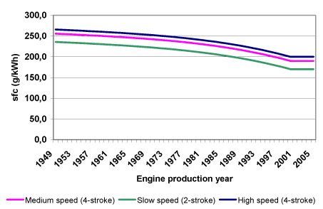
Figure 2.3 Specific fuel consumption for marine engines related to the engine production year (g/kWh)
Considering the fuel consumption trend graph in Figure 2.3, the first part of it applies to engines manufactured up until the mid 1990’s, and was produced in the late 1990s for the Danish TEMA 2000 model. Because the regression curve is supported by actual fuel consumption factors for these engines, this part of the graph is regarded as being the most accurate. For newer engines, the fuel consumption trend is established based on expert judgement. The graph is, however, still regarded as valid in relation to its use in estimating emission for engines in the situation which prevails today (pers. comm. Hans Otto Kristensen, DTU, 2006). The sfc figures for 2005 are used for engines built from 2006 onwards to provide the basis for the fuel consumption calculations for future years.
Using the average engine life times, LT, listed in Table 2.2, the average sfc factors per inventory year, X, is calculated from:
Where sfc = specific fuel consumption (g/kWh), X = inventory year, k = engine type, y = engine production year, LT = engine life time.
The average sfc factors per inventory year are shown in Figure 2.4 for the inventory years 2000-2020.
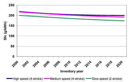
Figure 2.4 Average sfc factors for marine engines for the inventory years 2000-2020 (g/kWh)
2.7.2 NOx emission factors
2.7.2.1 IMO emission regulations for NOx
For seagoing vessels, NOx emissions are regulated as explained in Marpol 73/78 Annex VI, formulated by IMO (International Maritime Organisation), and further, amendments to MARPOL Annex VI has been agreed by IMO in October 2008. A three tiered emission regulation approach is considered, which comprises the following:
- Tier I: Diesel engines (> 130 kW) installed on a ship constructed on or after 1 January 2000 and prior to 1 January 2011.
- Tier II: Diesel engines (> 130 kW) installed on a ship constructed on or after 1 January 2011.
- Tier III[³]: Diesel engines (> 130 kW) installed on a ship constructed on or after 1 January 2016.
The NOx emission limits for ship engines in relation to their rated engine speed (n) given in RPM (Revolutions Per Minute) are shown in Table 2.3.
Table 2.3 Tier I-III NOx emission limits for ship engines (amendments to MARPOL Annex VI)
| NOx limit | RPM (n) | |
| Tier I | 17 g/kWh 45 x n-0.2 g/kWh 9,8 g/kWh |
n < 130 130 ≤ n < 2000 n ≥ 2000 |
| Tier II | 14.4 g/kWh 44 x n-0.23 g/kWh 7.7 g/kWh |
n < 130 130 ≤ n < 2000 n ≥ 2000 |
| Tier III | 3.4 g/kWh 9 x n-0.2 g/kWh 2 g/kWh |
n < 130 130 ≤ n < 2000 n ≥ 2000 |
Following the IMO emission regulations, the NOx Tier I limits are also to be applied for existing engines with a power output higher than 5000 kW and a displacement per cylinder at or above 90 litres, installed on a ship constructed on or after 1 January 1990 but prior to 1 January 2000.
2.7.2.2 NOx emission factors for engines built before 2006
The NOx emission factors (g/kWh) for slow- and medium-speed engines are obtained from MAN DIESEL (2006). With a global market share of 75%, MAN Diesel is by far the world’s largest ship engine manufacturer, and hence in terms of representativity, the emission factors are well suited as input for inventory emission calculations comprising many ships. For a relevant year of comparison, 2000, Winther (2008) finds a good accordance between the MAN Diesel emission factors and from other important studies (Whall et al. 2002; Endresen et al. 2003) per engine type. The concordance is the best for slow speed engines which is the most dominant source for NOx emissions.
The NOx emission factors provided by MAN Diesel for slow- and medium speed engines are shown in Figure 2.5, together with NOx emission factors for high-speed engines. For gas turbines, a mean NOx emission factor of 4 g/kWh is used. The emission information for high-speed engines and gas turbines comes from the Danish TEMA2000 emission model (Ministry of Transport, 2000). For high speed engines the emission factor level is determined by Kristensen (2006) through discussion with relevant engine manufacturers, considering engine operation at a normal engine speed range (1000 RPM) for high speed ferries. For high speed engines build in 2000, the NOx emission factor from Figure 3.4 fits with the IMO Tier I emission standard derived from the relevant equation in Table 3.2.
The increase in fuel efficiency up to year 2000 caused the NOx emission factors to increase. However, in the beginning of the 1990s (for slow-speed engines) and by the end of the 1990s (for medium-speed engines), NOx emission performance is improved, mainly due to improved engine design. The emission improvements are of a sufficient size to enable the IMO Tier I NOx emission requirements in 2000 to be met.
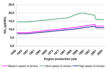
Figure 2.5 NOx emission factors for ship engines built before 2006 (g/kWh)
2.7.2.3 NOx emission factors for engines built from 2006 onwards
The Tier III requirements for new ships built after 2016 will apply in designated NOX Emission Control Areas (NECA). It is assumed that the AIS inventory area is appointed a NECA.
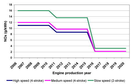
Figure 2.6 NOx emission factors for ship engines built from 2006 onwards (g/kWh)
Thus, for newer engines in compliance with Tier II (2011) and Tier III (2016) emission standards, emission factors are estimated by adjusting the Tier I emission factors (2000-2005) in two steps, relative to the Tier II:Tier I and Tier III:Tier I ratios. The estimated emission factors for the engine production years 2006-2020 are shown in Figure 2.6.
2.7.2.4 The effect of IMO NOx emission requirements for engines built from 1990 and prior to 2000
For slow speed engines, the new Tier I emission standards for existing engines built from 1990 to 1999 are somewhat lower than the emission factors actually measured by MAN Diesel. As mentioned in section 2.7.2.2, most of the ship engines today are built by MAN Diesel, and from their side it is expected that 75% of all slow speed engines built between 1990 and 1999 in the 7500-22500 kW segment will become retrofitted with more emission efficient slide valves in order to meet the IMO emission standards. Other engine sizes will also be considered at a later stage.
The slide valves are designed in a way which improves fuel atomization, penetration and mixing in the engine combustion chamber. On the same time engine performance adjustments are made (pers. comm. Michael F. Pedersen, MAN Diesel, 1999). The retrofit scheme is envisaged to take place following a linear time schedule from 1st of July 2011 to 1st of July 2016.
The retrofit emission effect is incorporated in the present inventory in similar way so that emission factors for 1990-1999 engine production years are gradually being replaced by Tier I emission factors, going from 0% to 100% representation between 1st of July 2011 and 1st of July 2016.
The correction factor KR is found as:
![]()
Where:
k = engine type (slow speed)
X = Inventory year, X = [2011;2020]
P = Main engine size (ME), P = [5000 kW;22500 kW]
y = engine production year, y = [1990;1999]
Outside the criteria for k, y, P and X, KR = 1.
2.7.2.5 Average NOx emission factors per inventory year
The average NOx emission factors take into account engine production year, average engine life times and the 2011-2016 retrofit scheme, as explained in the previous sections. It thus assumes that the sea area considered is appointed a NECA area, so Tier III regulations will apply after 2016.
Using the average engine life times listed in Table 2.2, the average NOx emission factors per inventory year, X, is calculated from:
Where EF = emission factor (g/kWh), X = inventory year, k = engine type, y = engine production year, LT = engine life time.
For the inventory years 2007, 2011 and 2020 the average NOx emission factors are shown in Annex II for ship category/engine type combinations, and with/without retrofit.
2.7.3 SO2
In relation to the sulphur content in heavy fuel and marine gas oil used by ship engines, Table 2.4shows the current legislation in force, and the amendment of MARPOL Annex VI agreed by IMO in October 2008. These sulphur contents are also used in the present inventory.
Table 2.4 Current legislation in relation to marine fuel quality
| Legislation | Heavy fuel oil | Gas oil | |||
| S-% | Impl. date | S-% | Impl. date | ||
| EU-directive 93/12 | None | 0.2¹ | 1.10.1994 | ||
| EU-directive 1999/32 | None | 0.2 | 1.1.2000 | ||
| EU-directive 2005/33² | SECA - Baltic sea | 1.5 | 11.08.2006 | 0.1 | 1.1.2008 |
| SECA - North sea | 1.5 | 11.08.2007 | 0.1 | 1.1.2008 | |
| Outside SECA’s | None | 0.1 | 1.1.2008 | ||
| MARPOL Annex VI | SECA – Baltic sea | 1.5 | 19.05.2006 | ||
| SECA – North sea | 1.5 | 21.11.2007 | |||
| Outside SECA | 4.5 | 19.05.2006 | |||
| MARPOL Annex VI amendments | SECA’s | 1 | 01.03.2010 | ||
| SECA’s | 0.1 | 01.01.2015 | |||
| Outside SECA’s | 3.5 | 01.01.2012 | |||
| Outside SECA’s | 0.5 | 01.01.2020³ | |||
| Notes: ¹Sulphur content limit for fuel sold inside EU ²From 1.1.2010 fuel with a sulphur content higher than 0.1 % must not be used in EU ports for ships at berth exceeding two hours ³ Subject to a feasibility review to be completed no later than 2018. If the conclusion of such a review becomes negative the effective date would default 1 January 2025 |
|||||
From 2006/2007[4], the SECA areas enter into force. The current inventory for 2007 assumes that the SECA regulations have been in place for the entire year of 2007, so a fuel sulphur content of 1.5% is used for heavy fuel oil in 2007. In 2011 and 2016 the sulphur content gradually become lower, as prescribed by the IMO fuel standards.
In order to obtain emission factors in g/kWh, the sulphur percentages from Table 2.5 are inserted in the following expression:
![]()
Where EF = emission factor in g/kWh, S% = sulphur percentage, and sfc = specific fuel consumption in g/kWh. The sfc factor is taken from equation 5.
Equation 1 uses 2.0 kg SO2/kg S, the chemical relation between burned sulphur and generated SO2 provided in EMEP/CORINAIR (2007).
2.7.4 PM
For diesel fuelled ship engines the emission of particles (primary particles - see Chapter 4 for details on secondary particles) depends on the fuel sulphur content, S%. The emission factors in g/kg fuel are calculated as:
![]()
The PM emission factor equation is experimentally derived from measurements made by Lloyd’s (1995). taken from TEMA2000 (Trafikministeriet, 2000).
Subsequently, the PM emission factor in g/kWh is found from:
![]()
Based on information from MAN DIESEL (N. Kjemtrup, 2006), the PM10 and PM2.5 shares of total PM (=TSP) are 99 and 98.5%, respectively.
The PM emission factors are experimentally derived from measurements made by Lloyd’s (1995). The latter source make up the basis for most of the inventories and methodology descriptions carried out so far on an international level, and hence the PM emission factors corresponds well with the input data used by e.g. the global inventories set up by Corbett and Koehler (2003) and Endresen et al. (2003), the inventory made for Europe by Whall et al. (2002), the European calculation methodology description from the MEET project (Georgakaki et al. 2004) as well as the EMEP/CORINAIR guidebook methodology (EMEP/CORINAIR 2009). The PM emission factors from Lloyds’ (1995) are also used in the Danish TEMA2000 emission model (Ministry of Transport, 2000).
2.7.5 CO and VOC
In general the emission factors for CO and VOC in g/kWh are regarded as very uncertain. The general experience from the ship engine manufacturer's side is a decrease in CO and VOC when fuel efficiency improves (pers. comm. S. Henningsen, MAN Diesel, 2006). However, due to missing consistent emission data as a function of engine year, constant factors for all engine production years are chosen for the present inventory. The emission factors originate from the emission measurement programme carried out by Lloyds (1995).
As for PM, the CO and VOC emission factors from Lloyd’s (1995) make up the basis for most of the inventories and methodology descriptions carried out so far internationally, and in this respect corresponds well with the emission factors used by e.g. the global inventories set up by Corbett and Koehler (2003) and Endresen et al. (2003), the inventory made for Europe by Whall et al. (2002), the European calculation methodology description from the MEET project (Georgakaki et al. 2004) as well as the EMEP/CORINAIR guidebook methodology (EMEP/CORINAIR 2009). One source however, Eyring et al. (2005), use factors which are considerably higher for VOC and somewhat lower for CO.
The CO and VOC emission factors from Lloyds’ (1995) are also used in the Danish TEMA2000 emission model (Ministry of Transport, 2000).
The CO and VOC emission factors are given in Table 2.5.
Table 2.5 CO and VOC emission factors
| Slow speed | Medium speed | High speed | Gas turbines | |
| (g/kWh) | (g/kWh) | (g/kWh) | (g/kWh) | |
| CO | 1.6 | 1.6 | 1.6 | 0.1 |
| VOC | 0.5 | 0.5 | 0.5 | 0.35 |
2.7.6 CO2
For CO2, the emission factors in g/kWh are calculated as:
![]()
The CO2 emission factors (g/MJ) are country specific (heavy fuel: 78 g/MJ; gas oil: 74 g/MJ) and come from the Danish Energy Authority (DEA). LHV = Lower heating value in MJ/kg (heavy fuel: 40.9; diesel: 42.7).
2.8 Calculation procedure
For each ship, the fuel consumption and emissions are found by summarising the product of engine load (%MCR), main engine size (kW), AIS signal time interval (s), and fuel consumption/emission factor (g/kWh):
![]()
Where E = fuel consumption/emissions (g), %MCR = engine load (%), Δt = sailing time between AIS signal (s), PME = main engine size (kW), EF = fuel consumption/emission factor in g/kWh, i = AIS signal interval, k = fuel type, l = engine type, X = calculation year.
The fuel consumption factor inserted in (12) is taken from (5), and the emission factors are taken from (7), (8) (10) and (11), for NOx, SO2, particulates and CO2, respectively, and Table 2.6 in the case of CO and VOC.
2.9 Results for fuel consumption and emission
The variation in fuel consumption totals for each month’s 48-hour period is shown in Figure 2.8 (c.f. Section 2.2). Some differences in the estimates appear from period to period, but the range of variations is moderate. Taking into account also the moderate fluctuations for number of ships present in the AIS inventory area for the same time periods (Figure 2.1), the conclusion is that a reasonably reliable full year inventory estimate can be obtained from the sum of the twelve periods by adjusting this sum with a multiplication factor of 365/24.
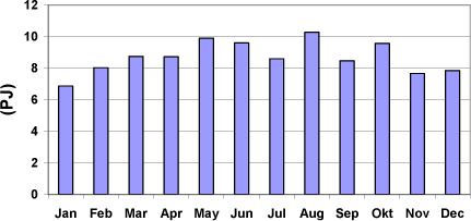
Figure 2.7 Fuel consumption from ships calculated using AIS data. Each column represents fuel consumption during a 48-hour period in the AIS inventory area (as depicted in Figure 1.1).
The resulting fuel consumption and emission estimates for the inventory years 2007, 2011 and 2020 are shown per ship type in Table 2.6. The presented results for the passenger Ro-Ro ship category consist of contributions from several vessel types, used for e.g. fishing, dredging research, towing/pushing and off shore activities (c.f. Annex 1).
Click here to see: Table 2.6 Fuel consumption and emissions per ship type
Figure 2.8 shows the fuel consumption and emission totals for the inventory years 2007, 2011 and 2020.
The 15 % increase in fuel consumption (and CO2 emissions) from 2007 to 2020 is a product of the envisaged growth in sea traffic and the gradually improved fuel efficiency for newer engines in historical years. The expected traffic growth for goods carrying vessels is around 36 % from 2007 to 2020, whereas sailing activities with passenger ships is expected to remain on the same level for the same period.
For SO2 and PM (all size fractions, primary particles) the reductions of the sulphur content lead to significant emission reductions. From 2007 to 2020[2011], the SO2 emission reductions are 91 % [36 %] whereas the PM reductions (all size fractions) are 54 % [31 %].
For NOx a marginal increase in total emissions of 2% is expected from 2007 to 2020. Without stricter emission standards the increase would have corresponded to the increase in fuel consumption, i.e. 15%. Thus, calculated on average the effect of IMO regulations is a reduction in the NOx emissions of 11% per unit of fuel. The reductions in the average NOX emission factor will continue after 2020.
The emission factors of VOC and CO are kWh based, and are assumed to be constant for all inventory years, and hence the increase in total emissions of around 25 % from 2007 to 2020 reflects the traffic projections.
In Figure 2.9 the calculated fuel consumption and emission shares of SO2, NOx and primary PM2.5 per ship type are shown for 2007, 2011 and 2020.
Today passenger ships is the largest source of fuel consumption and emissions of SO2 and primary PM2.5 (and CO2, CO and VOC; not shown) with shares of around one third of the calculated totals. However, from 2007/2011 these shares drop to one fourth in 2020, due to the underlying traffic composition in these years. As an end result, container ships become the largest source of fuel consumption and emissions in 2020.
For NOx, passenger ships, containers and tankers have almost the same emission shares in 2007 and 2011. However, due to the increase in traffic for goods transportation vessels from 2007/2011 to 2020, the relative fuel consumption and emission importance for container and tanker ships become larger than for passenger ships in 2020.
The fuel consumption and emission results are shown in even further details for the different ship type/fuel type combinations in Table 2.7.
In 2007 (and 2011) the calculated heavy fuel oil share of the total fuel consumption is 82 %. The corresponding emission shares are even higher being mostly pronounced for SO2 (97 %) and PM (92 %; all size fractions) due to the higher sulphur content for heavy fuel oil.
In 2020 the heavy fuel oil share has marginally changed to 81 %, but due to the significant reduction of the sulphur content for this fuel type, the emission shares of SO2 and PM2.5 become similar to those of fuel consumption.
Click here to see: Table 2.7 Fuel consumption and emissions per ship type and fuel type
In Figure 2.10 the fuel consumption and emissions of SO2, NOx and PM2.5 are shown as totals per flag state for the twelve 48 hour periods in 2007 that constitute the basis for the AIS inventory. The flag state nominations Denmark (DIS) and Norway (NIS) refer to ships included in secondary registers which a number of countries have established.
Open registers are essentially registers which have a loose interpretation of the link between a ship and the state whose flag it flies and which, accordingly, hold themselves "open" to ships from any country. They are subject to the same international rules as all flag states but they may offer beneficial tax arrangements. Standards of safety and environmental protection vary and are often subject to less strict control than under traditional national registers (pers. comm. E. Thompson, Lloyds Register, 2009).
Table 2.8 shows the data underlying Figure 2.10. The table lists percentage values and includes totals, grouped for EU countries and non-EU countries. It appears that 64% of the fuel consumption in the AIS inventory area can be attributed to ships from EU states.
Figure 2.10 Fuel consumption and emissions of SO2and NOx are shown as totals per flag state for the twelve 48 hour periods in 2007. The values refer to the AIS inventory area of Figure 1.1. The graph for PM2.5 resembles the SO2 graph and has been omitted.
2.10 Results: Spatial distribution
Figure 2.11 shows GIS based maps of fuel consumption and the emissions of SO2, NOx, VOC, CO, TSP, PM10, and PM2.5 for 2007, 2011 and 2020, respectively.
A general overview of the sea traffic around Denmark can be obtained by following the main passages of ships from east to west on the maps depicted in Figure 2.11.
From the inner Baltic Sea (Bothnian Bay), the main traffic passes through the waters between Bornholm and the south coast of Sweden. Considerable parts of the sea traffic go towards Lübeck/Kieler Kanal in Germany, or alternatively follow the shipping lane in the Great Belt strait between Zealand and Fuhnen. Another big part of the vessel movements are through the Øresund strait.
In Kattegat the two major shipping lanes unite (Anholt) and proceed to the tip of Jutland (Skagen). From this point most of the traffic passes south-west along the west coast of Jutland. Also very visible are the major Danish domestic ferry routes and the ferry routes connecting Denmark, Sweden, Germany and Poland.
In Figure 2.11, the previously explained emission developments from 2007 to 2020 are most visible for SO2 and PM2.5. As mentioned above, the emission reductions are due to the gradually lower sulphur content in the fuels used for navigation purposes.
Click here to see: Figure 2.11 - continued. Emissions of NOX, CO2 and VOC.
[2] Department of mechanical engineering, Section of coastal, maritime and structural engineering
[3] For ships operating in a designated Emission Control Area. Outside a designated Emission Control Area, Tier II limits apply.
[4] 2007 is used as the effective year in the inventory
3 Ship emission inventories for air pollution modelling
- 3.1 Introduction
- 3.2 "EMEP-ref" inventory
- 3.3 "AIS-2007" and "EMEP-2007" inventories
- 3.4 "AIS-sp" inventory
- 3.5 "AIS-2011" inventory
- 3.6 "AIS-2020" inventory
- 3.7 Summary of differences
3.1 Introduction
The previous chapter described how AIS-based inventories for ship emissions have been established. However, these data represent emissions for the AIS inventory area only (Figure 1.1). In order to apply the inventories in an air pollution model it is necessary to combine them with emission data covering a much larger geographical data.
The present chapter describes how the AIS-based data for ship emissions are combined with other ship emission data that cover a greater area. Some characteristics and differences between different inventories are also discussed. The chapter is entirely focussed on emissions from ships. Emissions from land-based sources are discussed in the subsequent chapter on air pollution modelling.
The following six emission inventories will be described and discussed:
EMEP-ref: Reference emission inventory based on the original ship emissions retrieved from the EMEP[5] database for 2006 with a spatial resolution of 50 km x 50 km (EMEP, 2008). Refers to the situation before SECA requirements for sulphur came into action. The EMEP inventory is based on an assumed sulphur content in residual oil of 2.7 % for several sea areas, including the North Sea and the Baltic Sea, following Cofala et al. (2007).
EMEP-2007: Emission inventory based on the above, but adjusted in order to represent conditions after the introduction of SECA. Emissions of sulphur and PM have been scaled down to reflect that introduction of SECA meant a reduction of sulphur content from 2.7 % to 1.5 %. No model runs have been performed for this inventory within the current project.
AIS-2007: Ship emissions based on AIS. Emissions for ships in SECA areas outside of the AIS inventory area have been scaled down to reflect that introduction of SECA meant a reduction of sulphur content from 2.7 % to 1.5 %. It has been assumed that the SECA regulations have been effective throughout the entire year of 2007.
AISsp-2007: Special version of the ship emissions based on AIS. This is a pre-SECA scenario. For the Danish marine waters AIS-based ship emissions are scaled up to the same total emission as those used in "EMEP-ref". The inventory is used to illustrate the effect of the improved spatial resolution of the ship emissions.
AIS-2011: Ship emission as AIS-2007, but projected to year 2011 based on the IMO-regulations and expectations on the development in the amount of ship traffic from 2007 to 2011. (All other emission sources are as for year 2007).
AIS-2020: Ship emission as AIS-2007, but projected to year 2020 based on the IMO-regulations, the assumption that the area considered is appointed a NOx Emission Control Area, and expectations on the development in ship traffic from 2007 to 2020. (All other emission sources have been projected to 2020 mainly based on the proposal for a new EU-directive for national emission ceilings in year 2020 - see Chapter 4).
The subsequent sections describe the inventories in more detail. They are used as basis for calculations of concentration levels, as described later in Chapter 4. Section 3.7 summarises differences between the inventories.
3.2 "EMEP-ref" inventory
In recent years, regional air pollution modelling work at NERI has been based on emission inventories where the information concerning ship emissions was based on a combination of two inventories: For a global coverage, the global ships emissions inventories of SO2, NOx, VOC, CO and PM by Corbett (see Wang et all, 2007) on a 0.1ox0.1ogrid was used. For the area around Europe the global ship emissions were replaced by emissions as estimated by EMEP for the year 2006 (latest reporting year; Cofala et al, 2007).
Figure 3.1 shows the emissions from ships based on these previous emissions inventories for the year 2006 for SO2, NOx, CO and PM2.5. The gridded EMEP emissions for the ships traffic (see Cofala et al., 2007) are based on an inventory of the emissions of marine activities that has been developed by ENTEC. This inventory is based on earlier estimates of emissions from ship movements between ports of the European Community that were compiled by Entec in 2002 and 2005 (see Whall et al, 2002, Entec 2005a-d). Emissions were estimated on the basis of vessel movement data and the underlying vessel emission factors as specified in Entec (2005a-d). The basis for this was four months of statistics obtained from Lloyds Marine Intelligence Unit (LMIU), which contains information about movements world-wide of ships, e.g. ships id, vessel type, engine type, Arrival/Departure Port/Place, Arrival/Departure Dates, etc. Based on the information on departure/arrival ports it is assumed that a vessel takes the shortest straight line route between two ports. When land prohibits this, the vessel takes the shortest route around the land towards the destination port. This procedure is used to establish the spatial distribution of emissions. Furthermore it is assumed that in open sea the engine load percentage is 80% of the maximum continuous rating (MCR), while in ports and during manoeuvring it is 20%. Concerning sulphur emissions, it is assumed that sulphur contents in residual oil is 2.7 percent (Cofala et al., 2007), and in marine distillates 0.2 percent.
The resolution of the air pollution transport model (DEHM) for the area around Denmark is 5.6 km. However, as seen on Figure 3.1 the resolution of the EMEP ship emissions is much cruder: 50 km. This means that over land close to the water there are ships emissions, which may result in an unrealistic contribution from ships emissions in these areas, as e.g. in Copenhagen and Aarhus. As also seen on the figure, the resulting ship emissions for the old emissions inventory assumes that most of the international ships traffic between the Baltic Sea and the North Sea passes through the Great Belt, probably because of the assumptions that are used to estimate the route for traffic between ports in the Baltic Sea and outside of it. The inventories shown in Figure 3.1 and the model runs based on these are called EMEP-ref.
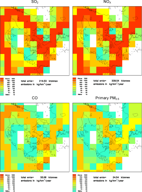
Figure 3.1 The original EMEP ship emissions for the year 2006 (called EMEP-ref). These are pre-SECA data. Upper left SO2 emissions, upper right NOx emissions, lower left CO emissions and lower right pm2.5 emissions. Note that although the labels say 2007 the inventory year is 2006 (pre-SECA).
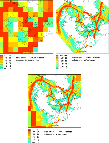
Figure 3.2 The EMEP-ref ship emissions of S02 (pre-SECA) are shown on the upper left, and the new AIS-based emissions of SO2 on the upper right. The lower figure shows how they are merged to form the post-SECA emission inventory called AIS-2007 as described in the text. The indicated totals represent the total for the area seen. They are not directly comparable to the totals given in the previous chapter.
3.3 "AIS-2007" and "EMEP-2007" inventories
Figure 3.2 illustrates how the emission inventories based on AIS data and the EMEP ship emissions are combined. The upper part of the figure shows the old SO2 EMEP ship emissions (the same as in Figure 3.1) and the new AIS-based emission inventory of SO2 based on the AIS data (corresponding to Figure 2.11), aggregated to 5.6 x 5.6 km resolution. These two inventories are merged to one single inventory. However, before merging them it should be taken into account that the EMEP-ref inventory represents data from before the SECA area became effective. EMEP-ref ship emissions are calculated with the assumption of a sulphur content of 2.7% in the residual oil. On the other hand, AIS emission data represent post-SECA conditions, where a sulphur content of 1.5% has been assumed.
The EMEP inventory can be adjusted for this by correcting the EMEP emissions of SO2 by a factor 0.563 and PM emissions by a factor 0.429. The corrected EMEP ship emissions are called EMEP-2007. Table 3.1 - Table 3.5 in section 3.7 summarise key values for the various emission inventories.
These two inventories - EMEP-2007 and the AIS-based - are merged to one single inventory by replacing the EMEP ship emissions with AIS emissions, where the AIS emissions cover an entire 50x50 km emissions grid or cover all ocean water. At the borders of the AIS area, where AIS emissions do not cover an entire grid cell, the AIS values and a residual value from EMEP are added. The residual is determined by an intelligent interpolation technique, which takes account of the EMEP emissions, the AIS emissions and the emissions in the neighbour grid cells of both EMEP and AIS emissions. The final result of this merging for the SO2 emissions is shown at bottom of Figure 3.2.
There are several interesting features about the new inventory. First, it has a much higher spatial resolution than EMEP-ref. There is not so much ship emission over land except in cities with large harbours. In the new inventory there is larger ship emissions in the Øresund compared to the EMEP inventories. Presumably this is because in the AIS data there are more ships passing through the Øresund as compared to the ENTEC data. This will be discussed further in section 3.7.
Another very important difference between the inventories is that total emissions are considerably lower according to the new inventory. Also this issue will be discussed in section 3.7.
Figure 3.3 shows the combined EMEP-2007 and AIS emission inventory for SO2, NOx, CO and PM2.5. This inventory is believed to be the most correct ship emission inventory for the year 2007 around Denmark. The inventory and the model runs based on it are called AIS-2007.
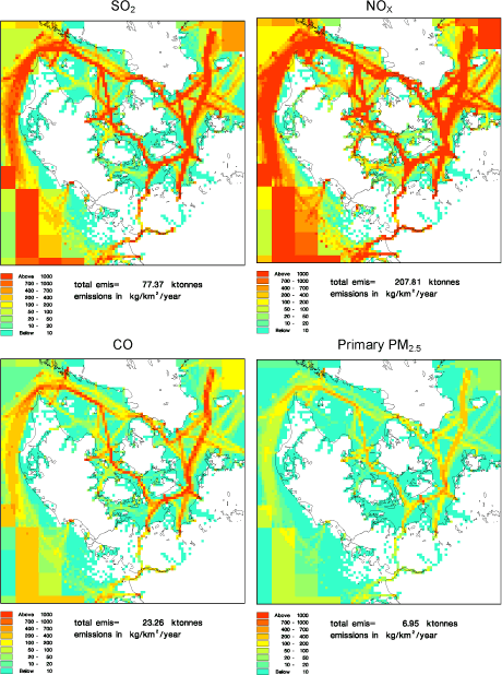
Figure 3.3 AIS-2007 inventory, representing post-SECA conditions. Formed by combing the AIS-based inventory with EMEP-2007 (a version of EMEP-ref where SO2 and pm2.5 emissions are scaled to reflect post-SECA conditions). Upper left SO2 emissions, upper right NOx emissions, lower left CO emissions and lower right pm2.5 emissions.
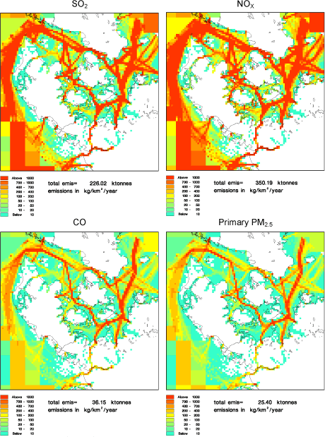
Figure 3.4 AIS-sp (special) inventory. The original EMEP ship emissions combined with AIS based emissions, which are scaled in order to have the total emissions as for the original EMEP ships emissions. The emission inventory is called AIS. Upper left SO2 emissions, upper right NOx emissions, lower left CO emissions and lower right pm2.5 emissions.
3.4 "AIS-sp" inventory
In order to investigate the differences caused by the finer resolution of the new emission inventories, as compared to the coarse EMEP inventory, a special inventory was established. The AIS emissions were scaled up in order to obtain the same total emission as the EMEP-ref ship emissions in Figure 3.1 (pre-SECA). This special inventory is shown in Figure 3.4 for four pollutants. The inventories and the model runs based on these are called AIS-sp (for special).
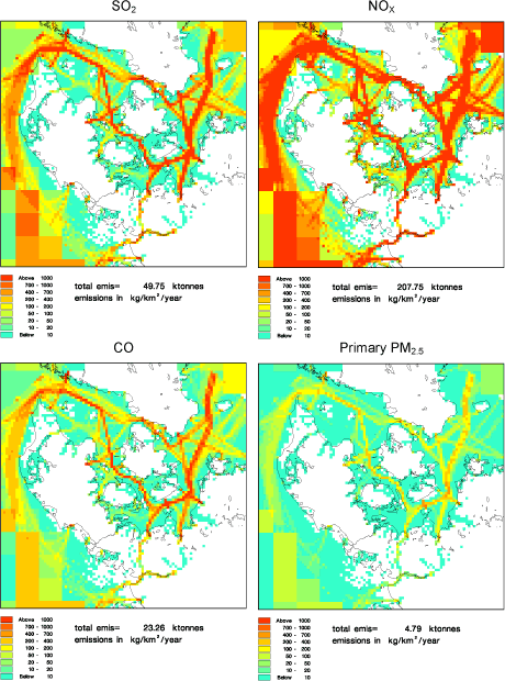
Figure 3.5 AIS-2011. The original EMEP ship emissions, where SO2 and pm2.5 emissions are scaled to the year 2011, combined with AIS based emissions for 2011. . Upper left SO2 emissions, upper right NOx emissions, lower left CO emissions and lower right pm2.5 emissions.
3.5 "AIS-2011" inventory
Figure 3.5 shows inventories for the year 2011. They are a combination of the AIS 2011 emission inventories and the EMEP-2007 inventories, where the EMEP SO2 emissions and PM emissions are multiplied with the ratio between emissions for 2011 and 2007 in the AIS inventories. For SO2 the ratio is 0.64 and for PM it is 0.69. In 2011 it is expected that emissions of SO2 and PM from ships will be about 30-35 % lower compared to the emissions in 2007. These inventories and the model runs based on these are called AIS-2011.
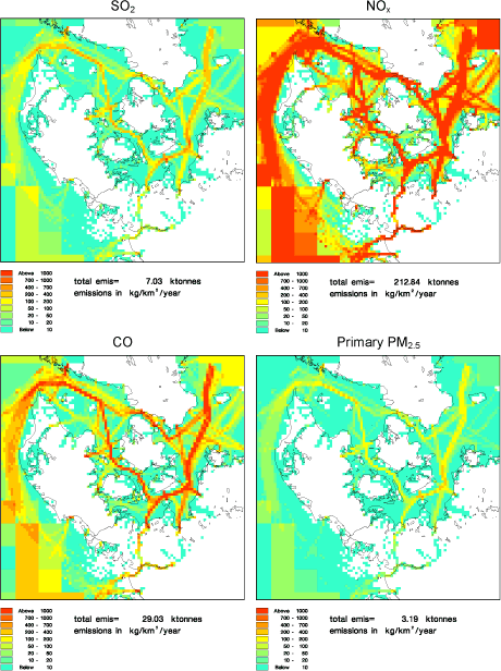
Figure 3.6 AIS-2020. The original EMEP ship emissions, where the emissions are scaled to the year 2020, combined with AIS based emissions for 2020. Upper left SO2 emissions, upper right NOx emissions, lower left CO emissions and lower right pm2.5 emissions.
3.6 "AIS-2020" inventory
Figure 3.6 shows inventories for the year 2020. They are a combination of the AIS 2020 emission inventories and the EMEP-2007 inventories, where all the EMEP emissions are multiplied with the ratio between 2020 and 2007 emissions in the AIS inventories. For SO2 the ratio is 0.09, for PM it is 0.46, for CO it is 1.25, for NOx it is 1.02, and for VOC 1.24. In 2020 it is expected that the SO2 emissions from ships will decrease by 91% compared to emissions in 2007, and PM emissions will decrease by more than 50%. The CO and VOC emissions will increase by 25% due to the expected increase in ship traffic, while the NOx will be nearly the same. These inventories and the model runs based on them are called AIS-2020.
3.7 Summary of differences
In Table 3.1 - Table 3.5 the emissions for the different marine waters around Denmark (the Baltic Sea West of Bornholm, Great Belt, Øresund and Kattegat) are summarized for the different emissions inventories used in the model calculations. Again the tables confirm that for the Øresund the new AIS emissions are higher than even the pre-SECA EMEP-ref inventory (with high sulphur content). If one compares the AIS-2007 emissions with the EMEP-2007 (both have the same sulphur content) one can see that the emissions for the Western Baltic Sea are nearly the same, whereas for the Great Belt and Kattegat the EMEP-2007 emissions are more than a factor of 2 higher; for the Øresund it is opposite. For the EMEP-ref inventory the total emissions in Great Belt are a factor of 11-12 higher than the total emissions in the Øresund, but for the AIS emissions it is only a factor of 2 higher, again indicating that the AIS data have more ship traffic through the Øresund relative to the Great Belt, compared to the data underlying the EMEP emissions.
When looking at the ENTEC report (Whall et al, 2002), which is the basis for the EMEP inventories, it seems that ENTEC has no ship movements through the Kiel Canal; instead, it assumes that these ships are taking a long route around Jutland to the North Sea through the Great Belt. In the AIS emission inventories there are emissions in the Kiel Canal (see Figure 3.3). This observed ship traffic through the Kiel-Canal will change the spatial distribution, so ship traffic is moved from the Great Belt and Kattegat to the Western Baltic Sea. This will also reduce the travel distance a lot, and therefore reduce fuel consumption and emissions in these areas. According to the official traffic statistic for Kiel-Canal, the total gross tonnage of the ships that passed through the Kiel-Canal from 2000 to 2007 has increased by 77% in the period (see http://www.kiel-canal.org/english.htm).
AIS-based emissions are generally lower than their EMEP counterpart, however with exceptions for some waters. One of the reasons for this difference is that EMEP always assumes that the engine load for the ships is 80% of the maximum in open sea, whereas for AIS-based emission inventories the engine load is estimated by using the actual speed of the ship.
The overall conclusion of the discussion above is that emissions based on the AIS data are expected to be better than the old EMEP inventory, because the AIS data have much more precise information of the different ships' location and speed compared to the crude assumptions made in the EMEP emission inventory. Furthermore, in Kattegat and Great Belt the AIS emissions are a factor of 2 smaller than the EMEP-2007 emissions, for the Western Baltic Sea they are very similar, and for the Øresund the AIS emissions are a factor 2 higher.
Table 3.1 SO2 emissions in kT SO2 for the different ocean waters and different inventories
| EMEP- ref |
EMEP- 2007 |
AIS- sp |
AIS- 2007 |
AIS- 2011 |
AIS- 2020 |
|
| Western Baltic Sea | 42.4 | 23.9 | 78.8 | 24.4 | 15.7 | 2.1 |
| Great Belt | 24.9 | 14.0 | 20.7 | 6.4 | 4.1 | 0.6 |
| Øresund | 2.3 | 1.3 | 9.0 | 2.8 | 1.8 | 0.3 |
| Kattegat | 41.0 | 23.0 | 35.5 | 11.2 | 7.2 | 1.0 |
| Area shown in Figure 3.2 etc. | 218 | 123 | 226 | 78 | 50 | 7 |
Table 3.2 NOx emissions in kT NO2 for the different ocean waters and different inventories
| EMEP- ref |
EMEP- 2007 |
AIS- sp |
AIS- 2007 |
AIS- 2011 |
AIS- 2020 |
|
| Western Baltic Sea | 67.2 | 67.2 | 110.3 | 58.5 | 58.7 | 59.2 |
| Great Belt | 39.1 | 39.1 | 34.3 | 18.2 | 18.1 | 18.2 |
| Øresund | 3.1 | 3.1 | 14.6 | 7.8 | 7.8 | 7.9 |
| Kattegat | 64.0 | 64.0 | 58.3 | 31.5 | 31.4 | 32.3 |
| Area shown in Figure 3.2 etc. | 340 | 340 | 350 | 208 | 208 | 213 |
Table 3.3 CO emissions in kT for the different ocean waters and different inventories CO
| EMEP- ref |
EMEP- 2007 |
AIS- sp |
AIS- 2007 |
AIS- 2011 |
AIS- 2020 |
|
| Western Baltic Sea | 6.8 | 6.8 | 12.3 | 7.3 | 7.3 | 8.8 |
| Great Belt | 4.0 | 4.0 | 3.3 | 1.9 | 1.9 | 2.4 |
| Øresund | 0.4 | 0.4 | 1.6 | 0.9 | 1.0 | 1.2 |
| Kattegat | 6.6 | 6.5 | 5.8 | 3.5 | 3.5 | 4.4 |
| Area shown in Figure 3.2 etc. | 35 | 35 | 36 | 23 | 23 | 29 |
Table 3.4 VOC emissions in kT for the different ocean waters and different inventories
| EMEP- ref |
EMEP- 2007 |
AIS- sp |
AIS- 2007 |
AIS- 2011 |
AIS- 2020 |
|
| Western Baltic Sea | 2.3 | 2.3 | 4.1 | 2.3 | 2.3 | 2.8 |
| Great Belt | 1.3 | 1.3 | 1.2 | 0.7 | 0.7 | 0.8 |
| Øresund | 0.1 | 0.1 | 0.5 | 0.3 | 0.3 | 0.4 |
| Kattegat | 2.2 | 2.2 | 2.0 | 1.1 | 1.1 | 1.4 |
Table 3.5 PM2.5 emissions in kT for the different ocean waters and different inventories
| EMEP- ref |
EMEP- 2007 |
AIS- sp |
AIS- 2007 |
AIS- 2011 |
AIS- 2020 |
|
| Western Baltic Sea | 4.8 | 2.0 | 8.8 | 2.2 | 1.5 | 1.0 |
| Great Belt | 2.8 | 1.2 | 2.4 | 0.6 | 0.4 | 0.3 |
| Øresund | 0.2 | 0.1 | 1.0 | 0.3 | 0.2 | 0.1 |
| Kattegat | 4.6 | 2.0 | 4.0 | 1.0 | 0.7 | 0.5 |
| Area shown in Figure 3.2 etc. | 24.5 | 10.5 | 25.4 | 6.9 | 4.8 | 3.2 |
[5] European Monitoring and Evaluation Programme. Full name: Co-operative Programme for Monitoring and Evaluation of the Long-Range Transmission of Air Pollutants in Europe.
4 Air pollution model calculations
- 4.1 Introduction
- 4.2 Interpreting PM2.5 results
- 4.3 Description of the model
- 4.4 Model runs and emission inventories
- 4.5 Results: Concentration levels
- 4.6 Contribution from ships
- 4.7 Comparison with measurements
- 4.8 Scenarios for 2011 and 2020
- 4.9 Concentration levels in Copenhagen
4.1 Introduction
This chapter describes the results from model calculations of the air pollution concentration levels in Denmark using the new and improved emission inventory for ships (AIS-2007). Chapter 2 explained how the ship emission inventory is constructed, and Chapter 3 how it is combined with other ship emission inventories to provide full hemispheric coverage for ship emissions.
The present chapter describes how the ship emissions are combined with emissions from land-based sources and aviation. However, the bulk of the chapter is devoted to a presentation and discussion of results for concentrations.
The model calculations include scenario calculations for the years 2011 and 2020. These scenario calculations are used to assess the effect that international regulations of ship emissions will have for the future air pollution in Denmark, while also taking into account the prospect for other emission sources. The international ship emission regulations were decided within the framework of the International Maritime Organisation (IMO), and are described in Chapter 2. It is important to note that the marine waters around Denmark are SECA areas, and that relatively strict requirements to the sulphur content in fuel apply (and have been assumed to apply for the entire year of 2007). Furthermore, it is assumed that these marine waters will be designated a NOX Emission Control Area (NECA), which will require an 80% reduction in NOX emissions for new ships after 2016.
The chapter contains the following parts:
- Section 4.2 is a brief introduction to interpretation of model results for PM2.5, as the reader should be aware of certain caveats.
- Section 4.3 describes the DEHM model which is used to estimate concentrations.
- Section 4.4 defines the emission inventories used. Previous chapters have discussed the inventories for ships near Denmark. This section sets them in a context where all other emissions sources are also considered.
- Section 4.5 discusses the results in terms of concentration levels for the current (2007) situation. It includes a discussion of the spatial distribution of concentrations, and also gives an overview of the concentration levels of the various pollutants for different regions in Denmark.
- Section 4.6 presents a very central set of results from the study: It quantifies the contribution from ships to the concentration levels in Denmark.
- Section 4.7 compares model results to measurements,
- Section 4.8 presents scenario calculations, demonstrating the combined effect on concentration levels of the IMO measures and the expected changes in land-based emissions.
- Section 4.9 discusses the influence of ship traffic on concentration levels in the Copenhagen area.
4.2 Interpreting PM2.5 results
The main focus during the evaluation of the influence of ship emissions on Danish air pollution has been on SO2, NO2 and primary PM2.5 (directly emitted fine particles). These are the major directly emitted pollutants from ship emissions. In addition to this there is focus on total PM2.5, since PM2.5 is considered to be strongly associated with negative human health effects.
When the results for PM2.5 are evaluated, it is important to bear in mind that PM2.5 consists of many different types of particles. In particular, it should be noted that PM2.5 calculated by the model consists only of primary PM2.5 and the secondary inorganic particles. These are the only parts of PM2.5 that are included in the model, and they account for only about half of PM2.5 in ambient air in Denmark. The remaining parts of the ambient PM2.5 including secondary organic particles are therefore not accounted for in the model calculations presented below. The reason for this is that there is not enough knowledge on the processes forming these secondary organic particles. This is also the case on international level (Yttri et al., 2009)
In order to clarify the distinction between total PM2.5 and the parts calculated by the model we will use the term mPM2.5 for the PM2.5 results from the model.
Measured values of PM2.5 in the ambient air will be higher than mPM2.5, because the measurements also include secondary organic particles. There is some further discussion on this issue later in the chapter, in particular in section 4.9.
4.3 Description of the model
The model calculations to assess air pollution concentration levels have been carried out with the Danish Eulerian Hemispheric Model (DEHM) which was developed at NERI. The model is used for the calculations in the Danish air quality monitoring programmes (Ellermann et al., 2009; Kemp et al; 2008) and has been used for almost a decade in connection with many research programmes carried out at NERI. The performance of the model has been tested in international model intercomparisons, where a high international standard has been confirmed.
DEHM is a Eulerian model that calculates emissions, transport, chemical and physical processes and deposition of air pollution in a three dimensional grid (Figure 4.1). The transport of the air pollution is determined on the basis of the meteorological conditions and takes place in and out of the individual grid cells in the horizontal as well as the vertical directions. Emissions are added to the model in the lowest layers of grid cells in the model. Low sources are added in the bottom layer while high stacks are added in the relevant layers of the model; typical at heights from 150 m to 600 m. The emissions from ships have been added to the bottom layers with an even distribution from the surface and up to 170 m height. This simple approach has been taken because of lack of more detailed information on the effective height of ship emissions.
Deposition of the air pollution is calculated from the concentrations in the lowest layers of the model. The deposited air pollutants are subsequently removed from these grid cells.
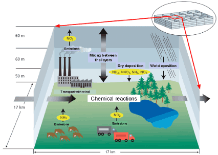
Figure 4.1 Illustration of the principles behind DEHM. For each grid cell the model calculates changes in the concentrations of the air pollutants due to emissions, transport with the wind, mixing between the layers, chemical and physical processes, and finally dry and wet deposition.
DEHM is designed with four different geographical domains with increasing spatial resolution:
- The first domain covers the entire northern hemisphere with a spatial resolution on 150 km x 150 km.
- The second domain covers Europe and some of the western Asiatic countries. This domain has a spatial resolution of 50 km x 50 km. The geographical area and the spatial resolution at this domain corresponds to area and resolution used in the model calculations carried out in connection to the European air monitoring programme EMEP.
- The third domain covers Denmark and the Danish marine areas plus some of the neighbouring countries. The spatial resolution is 17 km x 17 km.
- The fourth domain was recently introduced. It covers Denmark and parts of the Danish marine waters. This domain has a spatial resolution of approximately 6 km x 6 km. This high spatial resolution is needed in order to calculate properly the effects of ship emissions in the narrow Danish straits.
The four domains are shown in Figure 4.2. The four domains are linked in such a way that input data and results are dynamically exchanged between them. In this way the model can cover the entire northern hemisphere, and at the same time provide results for Denmark with a high spatial resolution. The ability to cover a large area and at the same time have high spatial resolution is especially important in this study. One of the reasons for this is that one of the major pollutants from ships is sulphur dioxide (SO2), which is chemically converted to particle bound sulphate (SO4²-) in the atmosphere. Sulphate is long range transported with typical travel distances of up to more than 1000 km. Hence the model needs to cover several thousand kilometres in all directions away from Denmark in order to capture all the sources that can have effect on the air pollution in Denmark. The fact that the Danish straits are typically 5-20 km wide illustrates the need for the high spatial resolution.
In the vertical direction the model covers the lowest 15 km of the atmosphere in 20 layers of grid cells. The lowest layers need the highest resolution and they have a thickness of about 60 m. The upper layers have a thickness of about 2000 m.
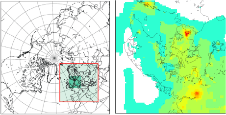
Figure 4.2 Left: The three first domains of DEHM. Right: Model calculated concentrations of sulphur dioxide in 2007 based on the fourth layer of the model. The small grid cells are 6 km x 6 km.
The meteorological input data needed for DEHM have been calculated using the meteorological model called MM5 (Grell et. al., 1995). It is part of the so-called THOR modelling system implemented at NERI (Thor.dmu.dk). All model calculations of air pollution in this project have been carried out using meteorological data for year 2007. In this way the only difference between the calculations for the reference year 2007 and the scenario calculations for 2011 and 2020 will be the changes in the emissions.
4.4 Model runs and emission inventories
Five different sets of model calculations have been carried out using different emission inventories in order to evaluate:
- the effect of the improvements in the emission inventories for ships;
- the contribution from ships to concentration levels;
- the effect of the international regulations aiming at a reduction of the ship emissions in the period up to 2020.
The emission inventories for SO2, NOX, VOC, CO and PM used for the five sets of model calculations are named as follows:
- EMEP-ref: Reference emission inventory based on the original ship emissions from EMEP[6] for 2006 with a spatial resolution of 50 km x 50 km (www.ceip.at). Refers to the situation before SECA requirements for sulphur became effective. Emissions from land-based sources and aviation for 2006 as described below.
- AIS-sp: Special version of the ship emissions based on AIS. This is a pre-SECA scenario. For the Danish marine waters AIS-based ship emissions are scaled up to the same total emission as those used in EMEP-ref. Other emissions are as described for EMEP-ref. The inventory is used to illustrate the effect of the improved spatial resolution of the ship emissions.
- AIS-2007: Ship emissions based on AIS. Emissions for ships in SECA areas outside of the AIS inventory area have been scaled down to reflect that introduction of SECA meant a reduction of sulphur content from 2.7 % to 1.5 %. It has been assumed that the SECA regulations have been effective throughout the entire year of 2007.
- AIS-2011: Ship emission as AIS-2007, but projected to year 2011 based on the IMO-regulations and expectations on the development in the amount of ship traffic from 2007 to 2011. All other emission sources are as for year 2007.
- AIS-2020: Ship emission as AIS-2007, but projected to year 2020 based on the IMO-regulations, the assumption that the area considered is appointed a NOX Emission Control Area, and expectations on the development in ship traffic from 2007 to 2020. All other emission sources have been projected to 2020 mainly based on EU’s thematic strategy on air pollution and projections from the International Institute for Applied Systems Analysis (see below).
Two model calculations have been carried out for each of the above mentioned emission inventories in order to determine the contribution from ships. One model calculation uses all the emissions, while the other is carried out with a 15 % reduction in all the ship emissions. The difference between these two model calculations enables us to determine the amount of air pollution originating from the ship emissions. This methodology has been preferred over another that might seem natural: To use a model run completely without ship emissions a as reference. Such an approach would, however, involve an unrealistic chemical regime, and its results could easily be misleading.
Details about the different inventories for the ship emissions have been described in Chapter 2 and 3. The emission inventories for the land-based emissions and aviation are briefly described in the following:
- Danish emissions for 2006 have been based on national emission inventories for NH3, NO2, SO2 and primary PM2.5 produced by NERI (Nielsen et al., 2008). For NH3 an inventory (by NERI) with a spatial resolution of 100 m x 100 m was used. This has subsequently been aggregated to a spatial resolution of 6 km x 6 km. For traffic emissions the spatial resolution is cells of 1 km x 1 km that are aggregated up to 6 km x 6 km. The remaining Danish sources have a spatial resolution of 17 km x 17 km. The inventory includes location and emissions for the most important Danish point sources (about 70).
- For the remaining part of Europe the emission inventories for 2006 have been based on national emissions inventories collected and distributed by EMEP (EMEP, 2008). These inventories for the total annual national emissions have subsequently been distributed to the 17 km x 17 km grid cells on the basis of a detailed international inventory from 1994 with high spatial resolution (Hertel et al., 2002).
- Emission data for the remaining part of the Northern hemisphere have been retrieved from the large international emission data base named EDGAR2000 Fast track, which is available with a spatial resolution of 1 x 1 degree.
For 2011 the emission scenario for land-based sources and aviation is based on the following:
- For Denmark and the rest of Europe it is assumed that the emissions are the same as in 2006. These emissions were assumed to be the best estimate of the emissions in 2011, that we had available at the time for the model calculations.
- For the remaining part of the northern hemisphere the projections of the emissions are based on the changes in the emissions due to current legislation and regulations of the emissions.
For 2020 the emission scenario for land-based sources and aviation is based on the following:
- For Denmark and the other 26 member states in EU the projections of the emissions are based on the emission scenario named “Thematic strategy on air pollution, central case” which has been defined by the International Institute for Applied Systems Analysis (Amann et al., 2008).
- For the remaining European countries and a number of the western Asiatic countries (corresponding to the countries covered by domain 2 in the model) the projections of the emissions are based on the projections made in the context of EU’s thematic strategy on air pollution (further described in Bach et al., 2006).
- For the remaining part of the northern hemisphere the projections for the emissions are based on current legislation and regulations of the emissions. These projections are based on the IIASA emission scenario for the year 2020 named “current legislation (CLR)” where the spatial resolution of 1 x 1 degree grid cells has been established by use of EDGAR emissions (Frank Dentener, JRC, personal communication, 2004).
Figure 4.3 shows a comparison of ship emissions according to three inventories. The emissions refer to Danish marine waters, as defined by the map on the right. These inventories were presented in Chapter 2 and the values are tabulated in Table 3.1, Table 3.2 and Table 3.5.
AIS-2007 represents the new NERI ship emission inventory. It comprises AIS-based ship emissions, while emissions outside of the AIS inventory area are downscaled (the scaling reflects SECA regulations). AIS-2007 is believed to be the most accurate inventory for the ship emissions in the Danish Marine Waters.
EMEP-ref is the original inventory from EMEP.
AIS-sp has deliberately been scaled in such a way that the total emissions are close to EMEP-ref. Hence the main difference between EMEP-ref and AIS-sp is the geographical resolution, which is 50 km x 50 km and 6 km x 6 km, respectively, and the spatial distribution of the ship traffic through the Danish marine waters.
It appears from Figure 4.3 that AIS-sp has higher emissions than AIS-2007. AIS-sp is 3.0, 1.7 and 3.5 times higher than AIS-2007 for SO2, NOX and PM2.5, respectively.
The differences between the inventories were further discussed in Chapter 3 and are mainly due to the following reasons:
- Only AIS-2007 assumes a sulphur content of 1.5%, corresponding to the conditions after the SECA requirements were introduced in 2006/7.
- AIS-2007 has more correct (and shorter) ship routes.
- AIS-2007 does not use the simplistic assumption that engine load is constant at 80%.
Figure 4.4 - Figure 4.6 illustrate the differences between emissions for the three scenarios 2007, 2011 and 2020, when considering emission from all sources. The figure is based on the inventories AIS-2007, AIS-2011 and AIS-2020. Each figure represents one pollutant (SO2, NO2 and PM2.5), while Table 4.1 lists results for all the emitted compounds. It appears that 2007 and 2011 differ only for the ship emissions in the North and Baltic Seas, while all other emissions are constant. On the other hand there are large differences between 2007 and 2020 for most of the areas and for the ship emissions in the North and Baltic Sea. It should be noted that for ship emissions of SO2 outside of SECA's, the computations do not take account of the reductions that will be introduced in 2020. The effect of these reductions will, however, not be large for concentrations in Denmark, because the seas around Denmark are SECA's, where stricter regulations apply. Further details on the emissions for all the air pollutants and the different scenarios for the ship emissions and the European countries are given in Appendix C.
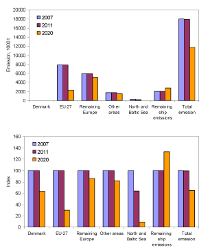
Figure 4.4 Emission of SO2 (top) and relative change of SO2 (bottom) for 2007, 2011 and 2020. Includes both land-based and marine emissions. The columns North and Baltic Sea represent the ship emissions for these two marine waters.
Figure 4.5 Emission of NOX (top) and relative change of NOX (bottom) for 2007, 2011 and 2020. The columns North and Baltic Sea represent the ship emissions for these two marine waters.
Figure 4.6 Emission of primary PM2.5 (top) and relative change of primary PM2.5 (bottom) for 2007, 2011 and 2020. The columns North and Baltic Sea represent the ship emissions for these two marine waters.
Table 4.1 Total emissions of NOX, NH3, SO2, CO, PM2.5, PMc0arse (PM10-PM2.5) and NMVOC (non methane volatile organic compounds). The columns North and Baltic Sea represent the ship emissions for these two marine waters
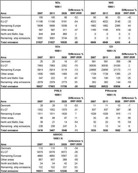
4.5 Results: Concentration levels
Figure 4.7 to Figure 4.10 show maps with results of the model calculations for concentration levels of SO2, NO2, primary PM2.5 and mPM2.5 (defined in section 4.2), using the three different ship emission inventories (EMEP-ref, AIS-sp and AIS-2007). It is clearly seen that there are major differences between the results using the three different inventories, both with respect to spatial distribution and the concentration levels.
In the following subsections, characteristics and differences between the three sets of results will be discussed. Readers who are mainly interested in the most accurate results should focus on results based on AIS-2007.
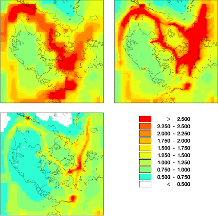
Figure 4.7 Model results for SO2 concentration levels using EMEP-ref (upper left), AIS-sp (upper right), and AIS-2007 (lower left) in units of µg/m³.
4.5.1 Spatial resolution
The major differences between the spatial distribution of the ship emissions are clearly reflected in the concentration maps for concentrations of SO2 and NO2 (Figure 4.7 and Figure 4.8). For primary PM2.5 and mPM2.5 the differences are less evident.
The reason for the large differences in the spatial distribution was described in depth in Chapter 3. Briefly, the original EMEP-ref emission inventory was based on information about which ports the ships were sailing from and to, while there was no information on the actual sailing routes. Erroneously a too large fraction of the ships was assumed to pass through the Great Belt compared to the Øresund. The AIS-sp and AIS-2007 inventory have been based on information on the actual sailing routes (Chapter 2 and Chapter 3). These two inventories give therefore a much more accurate representation of the spatial distribution of the emissions, and the results from use of these emission inventories are therefore also more accurate.
Another interesting result is the effect of the increase in spatial resolution from 50 km x 50 km (EMEP-ref) to 6 km x 6 km (AIS-sp and AIS-2007). In the results from the model calculations using EMEP-ref the large grid cells are clearly apparent (Figure 4.7 and Figure 4.8). Moreover, for SO2 concentrations it can be seen that the grid cells containing emissions from ships are actually covering land areas, leading to a significant overestimation of the air pollution with SO2 in these areas (Figure 4.7). In the results for SO2 concentrations based on AIS-sp and AIS-2007 the ship routes appear more distinct, in agreement with the fact that the majority of the ship traffic is confined to quite narrow ship routes through the Danish marine waters. Similar improvements also apply for NO2 and primary PM2.5.
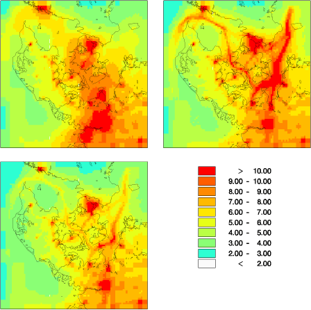
Figure 4.8 Model results for NO2 concentration levels using EMEP-ref (upper left), AIS-sp (upper right) and AIS-2007 (lower left) in units of µg/m³.
Figure 4.9 Model results for primary PM2.5 concentration levels using EMEP-ref (upper left), AIS-sp (upper right), and AIS-2007 (lower left) in units of µg/m³.
The spatial distribution for mPM2.5 (Figure 4.10) is completely different from SO2, NO2 and primary PM2.5 (Figure 4.7 to Figure 4.9). The reason for this is twofold. First, PM2.5 consists of particles with a long atmospheric lifetime. Hence, mPM2.5 is long range transported. Secondly, the ship emissions contribute only with less than 20% to mPM2.5 (cf. Section 4.6) while sources in the countries south of Denmark are responsible for the main part of mPM2.5 in Denmark. Altogether, this leads to a gradient with decreasing mPM2.5 going from South to North. This gradient dominates the spatial distribution of mPM2.5, and the sailing routes are only visible in Kattegat in AIS-sp.
Figure 4.10 Model results for mPM2.5 concentration levels (only primary and secondary inorganic particles) using EMEP-ref (upper left), AIS-sp (upper right), and AIS-2007 (lower left) in units of µg/m³.
In general for all compounds, the concentration levels are more or less the same when comparing results where either EMEP-ref or AIS-sp is the underlying inventory, whereas concentrations are lower when AIS-2007 is used (Figure 4.7 - Figure 4.10). This is to be expected since the total emissions from ships in the Danish marine waters are set to the same values in EMEP-ref and AIS-sp, while the ship emissions are considerably lower in AIS-2007 (Figure 4.3).
As noted before, the lower emissions in AIS-2007 are caused by the fact that the inventory takes account of the SECA-regulations, combined with improvements in the inventory itself (e.g. more accurate sailing routes), and better assumptions behind calculations of the emissions (cf. Chapter 2).
4.5.2 SO2 concentration levels by region
Figure 4.11 and Table 4.2 give an overview of the average concentrations for SO2, NO2, primary PM2.5 and PM2.5 (only primary and secondary inorganic particles) for the Danish regions and for Denmark using the three different emission inventories. Thus, it summarises information from the maps of the previous section.
For SO2 there are large differences between the average concentrations for the different regions. This is because ship emissions are a major source of SO2 in Denmark (see section 4.6) and because of the uneven spatial distribution of the ship traffic. This leads to high emissions of SO2 in the waters around Zeeland and close to Copenhagen. In addition the land-based emissions of SO2 are largest in Copenhagen and Zeeland. This leads to the highest concentrations in Copenhagen and Zeeland and the lowest concentrations in the Middle Jutland. EMEP-ref and AIS-sp resemble each other in respect to region-wise concentration levels. The lower ship emissions in AIS-2007 result in a reduction in the average modelled SO2 concentrations, compared to the results based on the original ship emissions from EMEP (EMEP-ref) of 36-51%; for Denmark in average the reduction is 44%. The reductions in the concentrations are nearly as high as the 64% reduction of the ship emissions from EMEP-ref to AIS-2007.
4.5.3 NO2 concentration levels by region
For NO2 a very similar pattern to that of SO2 can be seen with the highest concentrations in Copenhagen and Zeeland and the lowest concentrations in North and Middle Jutland. This complies with the location of the main NO2 sources that are land-based combustion sources, while ship traffic contributes with about 1/5 to the concentrations of NO2 (cf. section 4.6). The change from EMEP-ref to AIS-2007 leads to a reduction in the modelled NO2 concentration in the different regions of 7-20%; for Denmark in average 13%. This is about a third of the 39% reduction in the ship emissions from EMEP-ref to AIS-2007 and agrees well with the fact that about 1/5 of the NO2 concentration originates from ship traffic.
4.5.4 PM2.5 concentration levels by region
For primary PM2.5 and mPM2.5 there are only minor differences between the regions. This is because of the long atmospheric lifetime of PM2.5 that leads to more evenly distributed concentrations of PM2.5 and mPM2.5, as compared to SO2 and NO2. Moreover, only a minor part (about 10-20%) of mPM2.5 originates from ship emissions (cf. section 4.6) and hence there is only a 9-16% change in concentrations of mPM2.5 for the various regions when EMEP-ref is compared with AIS-2007; for Denmark in average the reduction is 10%. This is despite the fact that the emissions of primary PM2.5 from ships are reduced by 72% going from EMEP-ref to AIS-2007.
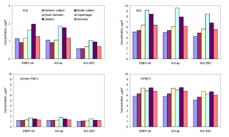
Figure 4.11 Model calculated average concentrations for SO2, NO2, primary PM2.5 and mPM2.5 (only primary and secondary inorganic particles) for the Danish regions and Denmark using EMEP-ref, AIS-sp, AIS-2007. Note that the values for Copenhagen refer for the entire Copenhagen region and therefore differ from the urban background in the centre of Copenhagen.
Table 4.2 Model calculated average concentrations in µg/m³ for SO2, NO2, primary PM2.5 and mPM2.5 (only primary and secondary inorganic particles) for the Danish regions and Denmark using EMEP-ref , AIS-sp, AIS-2007.
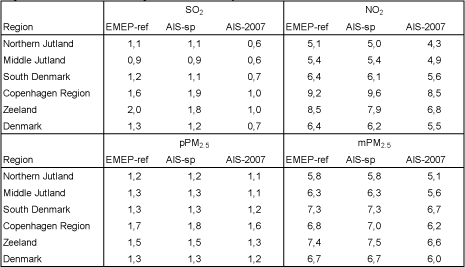
4.6 Contribution from ships
As explained in section 4.4 the contribution to air pollution from ships can be estimated by comparing results of two model calculations: one with ship emissions, and the other with reduced ship emissions. Figure 4.12 shows results for the relative contribution from ships according to the three inventories under discussion. Table 4.3 contains the corresponding values.
For all the compounds it can clearly be seen that the difference between EMEP-ref and AIS-sp is small, since the improved spatial distribution for the ship emissions does not lead to significant changes for the concentration levels in Denmark in average. However, there is a large difference between results based on EMEP-ref and on AIS-2007 due to the lower ship emissions in AIS-2007.
As explained before, AIS-2007 is considered as the most reliable inventory. Based on AIS-2007 it is seen that the largest contribution from ship emissions is for SO2, where 37% of the average concentration is due to ship emissions. For the other compounds the contribution to concentration levels from ship emissions lies in the range from 18-23% except for primary PM2.5 where the contribution is as small as 6%.
For mPM2.5 as an average over Denmark, the contribution from ships is estimated to be around 18% based on AIS-2007. This result can not be interpreted to say that ship pollution is responsible for 18% of the particle pollution in Danish ambient air, because mPM2.5 is only a part of the total PM2.5 found in the atmosphere. Some further considerations along this line can be found in section 4.9. It can be noted that based on the previous inventories the relative contribution from ships to mPM2.5 was 25%
The changes in the ship emissions also have an impact on ammonia (NH3) and particulate ammonium (NH4+) although they are not emitted from ships. When the level of SO2 is reduced NH3 increases and NH4+ decreases. This is due to the large changes in the ship emissions of SO2 and the chemical reactions between sulphur compounds and ammonia and ammonium:
SO2 –> –> –> H2SO4
H2SO4 + NH3 –> NH4HSO4
NH4HSO4 + NH3 –> (NH4)2SO4
The large decrease in the concentrations of SO2 leads to formation of less sulphuric acid (H2SO4) which again slows down the reaction between H2SO4 and NH3, leading to formation of particulate NH4+ in form of ammonium bisulphate (NH4HSO4) and ammonium sulphate ((NH4)2SO4). Hence the reductions in the relative contribution from ship traffic to SO2 due to change from EMEP-ref to AIS-2007 leads to a minor increase in NH3 and a decrease in NH4+.
Table 4.3 Corresponds to Figure 4.12. Relative contribution from ship emissions to the average concentrations of selected air pollutants in Denmark in 2007 with three different emission inventories.
| SO2 | SO4²- | NO2 | SNO3 | NH3 | NH4 | pPM2.5 | mPM2.5 | |
| EMEP-ref | 68% | 33% | 32% | 24% | -10% | 25% | 18% | 25% |
| AIS-sp | 66% | 36% | 30% | 26% | -9% | 25% | 16% | 25% |
| AIS-2007 | 37% | 21% | 21% | 23% | -6% | 18% | 6% | 18% |
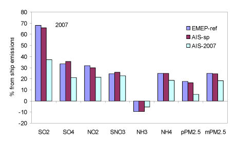
Figure 4.12 Relative contribution from ship emissions to the average concentrations of selected air pollutants in Denmark in 2007 with the three different emission inventories EMEP-ref, AIS-sp, and AIS-2007. SO4 is SO4²-. pPM2.5 is primary PM2.5. mPM2.5 is the model calculated PM2.5. SNO3 is the sum of nitric acid (HNO3) and particulate nitrate. The negative values for NH3 occur because reductions in SO2 from ships lead to an increase in NH3. This is a consequence of the way the contribution from ships is calculated
4.7 Comparison with measurements
A comparison between model calculations and measurements has been carried out in order to validate the results of the model calculations using the new ship emission inventories. The results from this comparison can be seen in Figure 4.13 for some of the main compound of interest in relation to ship emissions.
For SO2 the change to the AIS-2007 emission inventory for ships has lead to major reductions in concentration values modelled for the Danish monitoring stations, thereby causing a significant improvement of the model calculations. The improvement is most dramatic for the two coastal monitoring stations Anholt and Keldsnor where the change from EMEP-ref to AIS-2007 has resulted in a reduction in calculated SO2 concentration by a factor of 3 and 2, respectively. However, also for the inland monitoring station Tange there is a significant reduction by a factor of 1.5. The results from use of the new ship emission inventory (AIS-2007) are in very good agreement with the measurements, while use of the original inventory EMEP-ref resulted in significant overestimation of SO2.
For NO2, particulate SO4²- and secondary inorganic particles there are only minor changes between the results obtained from the use of the three different emission inventories. In general, use of AIS-2007 has resulted in a reduction of the concentrations of only about 10-36% compared to EMEP-ref.
For NO2, particulate SO4²- and secondary inorganic particles, EMEP-ref is in general in better agreement with the measurements than AIS-2007. However, despite this AIS-2007 is still in good agreement with the measurement results. For NO2 the differences between model calculations using AIS-2007 and measurements are 7-32%, for particulate SO4²- the differences are 24-34% and for secondary inorganic particles the differences are 23-31%.
The minor worsening for NO2, particulate SO4²- and secondary inorganic particles is believed to be secondary to the major improvements for SO2. It is therefore concluded that the newly developed emission inventory AIS-2007 is a significant improvement compared to the original emission inventory from EMEP (EMEP-ref). Use of the original ship emissions from EMEP (EMEP-ref) leads therefore to model results with too high concentrations of SO2 for Denmark.
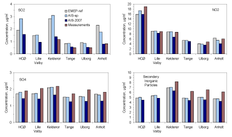
Figure 4.13 Comparison between results from model calculations and measurements for the concentrations of SO2, NO2, particulate SO4²- and secondary inorganic particles in 2007 at selected Danish monitoring stations. Model calculations are carried out using the three different emission inventories EMEP-ref, AIS-sp and AIS-2007. SO2 and secondary inorganic particles are not measured at HCØ and Lille Valby
4.8 Scenarios for 2011 and 2020
The results of the model calculations for 2007 and the scenario calculations for 2011 and 2020 are shown in Figure 4.13 to Figure 4.17 for SO2, NO2, primary PM2.5 and PM2.5, respectively. All three sets of model calculations are carried out using meteorology from year 2007, so that the only difference between the years is the difference in the emissions. The emission inventories for the ship emissions are all based on AIS-2007 that has been scaled to 2011 and 2020 based on the expected changes in ship traffic intensity and effect of the IMO regulations of the emissions from ships (see Chapter 3). The basis for the scenarios for the emissions from land-based sources and aviation in 2011 and 2020 is explained in Chapter 1.3.
4.8.1 SO2 concentration levels - future scenarios
For SO2 concentrations, the scenario calculations show that there will be a decrease of about 13% between 2007 and 2011. The SO2 concentration will continue to decrease up to 2020, so that the overall change from 2007 to 2020 is about 62% in terms of concentrations. The decrease is approximately the same for all the Danish regions (Figure 4.18). From 2007 to 2020 a 90 % reduction is expected for the ship emissions of SO2 in both the North Sea and Baltic Sea, and it is evident that this large reduction contributes substantially to the reduction in the SO2 level. This can also be seen directly from Figure 4.14, where the distinct SO2 signal from the sailing routes in 2007 disappears in 2020. However, from 2007 to 2020 a 70% emission reduction is expected for the land-based sources of SO2 in EU-27, and this reduction will also contribute substantially to the reduction in SO2. In 2020 the average Danish SO2 concentration is expected to be only 0.3 µg/m³, corresponding to only about 6% of the average concentration measured in 1990 at the Danish monitoring stations in the Danish background monitoring programme (Ellermann et. al., 2009). Moreover, the average concentration is as little as 1.5% of the EU limit value for protection of vegetation, and the concentrations will also be far below the limit values for protection of human health (EU directive 2008/50/EF).
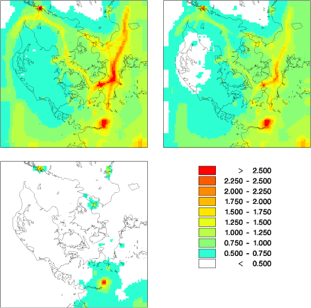
Figure 4.14 Model results for SO2 using AIS for 2007 (upper left), 2011 (upper right) and 2020 (lower left) in units of µg/m³.
4.8.2 NO2 concentration levels - future scenarios
The development for NO2 is somewhat different from SO2 since the average ship emissions for NOx in the North and Baltic Sea is expected to remain essentially unchanged from 2007 to 2020. The change in the average Danish NO2 concentrations is therefore smaller than for SO2. From 2007 to 2011 no change is calculated, but from 2007 to 2020 a reduction of 36% is expected for the average concentration of NO2 for all the Danish regions (Figure 4.18). This reduction is mainly driven by a 50% reduction in the land-based NO2 sources in Denmark and in the remaining EU-27. That it is the land-based sources that causes the reductions in NO2 and not the ship traffic, can also be seen from Figure 4.15. The Danish highways are clearly seen in 2007 but disappear in 2020, while the sailing routes are visible both in 2007 and 2020.
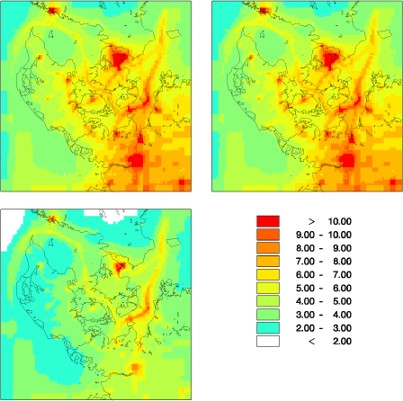
Figure 4.15 Model results for NO2 using AIS for 2007 (upper left), 2011 (upper right) and 2020 (lower left) in units of µg/m³.
4.8.3 PM2.5 concentration levels - future scenarios
For primary PM2.5 a 2% reduction in concentrations is expected from 2007 to 2011 solely due to a 30% reduction in ship emissions of primary PM2.5 in the North and Baltic Sea. During the period from 2007 to 2020 a 34% reduction of primary PM2.5 is expected for all the Danish regions (Figure 4.18). The reductions in primary PM2.5 are mainly caused by 50% reductions in the ship emissions from the North and Baltic Sea and from land-based sources in Denmark, as well as a 30% reduction in emissions from the remaining EU-27.
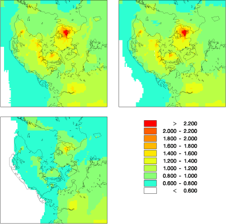
Figure 4.16 Model results for primary PM2.5 using AIS for 2007 (upper left), 2011 (upper right) and 2020 (lower left) in units of µg/m³.
For mPM2.5 (defined in section 4.2) only a 3% reduction in concentration level is expected from 2007 to 2011 (Figure 4.17 and Figure 4.18). This is due to reductions in ship emissions of primary PM2.5 and SO2 (Table 4.1). SO2 leads to formation of particulate sulphate that is one of the components of secondary inorganic particles. During the period from 2007 to 2020 a 39% reduction of mPM2.5 is expected for all the Danish regions (Figure 4.18). The reductions in mPM2.5 are mainly caused by reductions in the ship emissions from the North and Baltic Sea, land-based sources in Denmark and reductions in land-based emissions from the remaining EU-27.
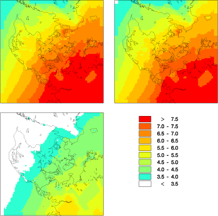
Figure 4.17 Model results for mPM2.5 (only primary and secondary inorganic particles) using AIS for 2007 (upper left), 2011 (upper right) and 2020 (lower left) in units of µg/m³
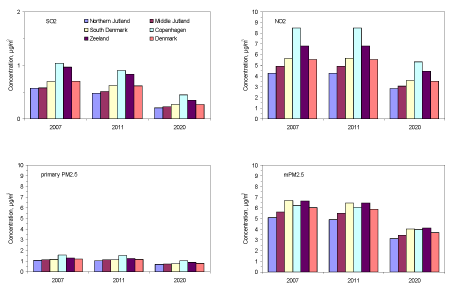
Figure 4.18 Average concentrations for the Danish regions for SO2, NO2, primary PM2.5 and mPM2.5 (only primary and secondary inorganic particles) using AIS for 2007, 2011 and 2020. Note that the values for Copenhagen refer to the entire Copenhagen region and therefore differ from the urban background in the centre of Copenhagen.
Table 4.4 Average concentrations for the Danish regions in µg/m³ for SO2, NO2, primary PM2.5 and mPM2.5 (only primary and secondary inorganic particles) using AIS for 2007, 2011 and 2020.
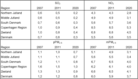
4.8.4 Contribution from ships according to the scenarios
As explained in section 4.4 the contribution to air pollution from ships can be estimated by comparing results of two model calculations: one with ship emissions, and the other with reduced ship emissions.
Figure 4.19 and Table 4.4 shows the average annual concentrations for Denmark calculated for 2007 and as expected for 2020. For the sulphur compounds the main change from 2007 to 2020 is a decrease due to the regulations of the ship emissions. For NO2 and the sum of particulate nitrate and nitric acid there are also large reductions. However, these reductions are due to expected regulations of the land based sources. Also for the particles (primary PM2.5 and mPM2.5) the reductions are mainly due to reductions of land-based sources. However, for the particles minor reductions are also seen for the ship emissions.
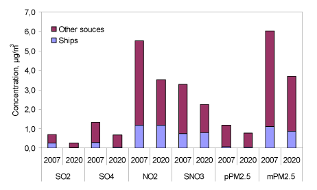
Figure 4.19 Average annual concentrations for Denmark for 2007 and 2020 divided in contribution from ships and other sources. SO4 is SO4²-. pPM2.5 is primary PM2.5 and SNO3 is the sum of nitric acid (HNO3) and particulate nitrate. Finally mPM2.5 is the part of PM2.5 included in the model.
Table 4.5 Average annual concentrations in µg/m³ for Denmark for 2007 and 2020 divided in contribution from ships and other sources. SO4 is SO4²-. pPM2.5 is primary PM2.5 and SNO3 is the sum of nitric acid (HNO3) and particulate nitrate. mPM2.5 is the part of PM2.5 included in the model.
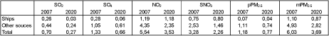
Figure 4.20 shows the development in the relative contribution to air pollution originating from ship emissions. Large reductions in concentration levels are expected for SO2 (37%?10%) and SO4²- (21%?9%), when going from 2007 to 2020. This is due to the 91% reduction of the emissions from ships in the North and Baltic Sea. This reduction is larger than the reductions in other sources (Table 4.1) and hence there is a decrease in the relative amount of SO2 and SO4²- originating from ship traffic.
For NO2 (21%?34%), HNO3+NO3 (23%?35%), and PM2.5(18%?23%) the relative amount originating from ship emissions is expected to increase in the period from 2007 to 2020 (Figure 4.20). This is because the land-based sources are reduced more than the ship emissions (Table 4.1). For primary PM2.5 (6%?5%), there is practically no change in the relative amount originating from ship emissions because land-based sources in Denmark and EU-27 and ship emissions are reduced with approximately the same fraction (Table 4.1).
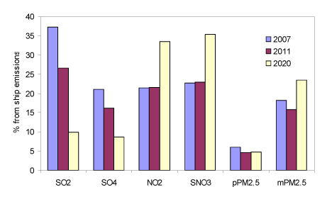
Figure 4.20 Relative contribution from ship emissions to the average concentrations of selected air pollutants in Denmark in 2007, 2011 and 2020 based on AIS. SO4 is SO4²-. pPM2.5 is primary PM2.5 and SNO3 is the sum of nitric acid (HNO3) and particulate nitrate. mPM2.5 is the part of PM2.5 included in the model.
4.9 Concentration levels in Copenhagen
The influence of ship traffic to the general level of air pollution in the Copenhagen area has also been investigated within the current project. The reason for this is that there are problems with too high air pollution levels of NO2 and PM2.5 in the Copenhagen area and that the intensity in the ship traffic in Øresund is high. Figure 4.21 shows the model calculated concentrations for SO2, NO2 and mPM2.5 at the urban background station at the H.C. Ørsteds Institute in Copenhagen and at the rural background station Lille Valby about 30 km west of Copenhagen.
For SO2 concentration a significant reduction can be seen when going from 2007 to 2020 at both stations. It is also clearly seen that the amount of SO2 coming from ship traffic is significant in 2007 and that the IMO regulations of the emissions of SO2 from ships is expected to reduce the contribution from ships to a very low value.
For NO2 there is similarly a marked decrease in the NO2 concentration at both stations from 2007 to 2020. However, the absolute amount of NO2 coming from ships remains constant, whereas the reductions from the land-based sources are responsible for the reduction in the NO2 concentration. The contribution from ship traffic to the urban background concentration of NO2 is therefore expected to change from 12% in 2007 to 21% in 2020. In a longer time perspective the contribution from ships can be expected to decrease, at least in absolute terms, because of strict requirements to NOX emissions implemented for new ships from 2016.
It is interesting to note that for the urban background the NO2 concentration is expected to decrease from about 16 μg/m³ in 2007 to about 9 μg/m³in 2020. This reduction in urban background NO2 will reduce the problems with exceedances of the EU limit values for NO2 in Copenhagen.
For mPM2.5 the situation is much the same as for NO2. A considerable change in concentrations takes place from 2007 to 2020, but there is only a barely visible change in the amount of mPM2.5 coming from ship emissions. Both values are small: 0.9 μg/m³ in 2007 and 0.7 μg/m³ in 2020. It should be recalled that the concentration values represented in Figure 4.21 are for the model calculated PM2.5 - mPM2.5 - which only includes primary PM2.5 and secondary inorganic particles, but not secondary organic particles. It is therefore interesting to compare with measurements of ambient PM2.5.
In 2007 the only measurements of PM2.5 were carried out at the street station at H.C. Andersens Boulevard in Copenhagen. Here the annual average concentration of PM2.5 was measured to 23 µg/m³ (Kemp et al., 2008).
The amount of primary PM2.5 and secondary inorganic particles originating from ships will to a good approximation be the same in urban background (HCØ) and at street level (H.C. Andersens Boulevard). According to the model calculations the ship contribution to this sum is approximately 0.9 μg/m³. Thus, the relative contribution from ships to pollution with PM2.5 in a busy street in Copenhagen - H.C. Andersens Boulevard in 2007 - can be estimated to 4% of total PM2.5.
In the urban background the relative contribution from ships is larger. The concentration of PM2.5 in urban background in Copenhagen (HCØ) was not measured until 2008. Here the concentration was measured to 13 µg/m³ (Kemp et al., 2009). Based on this it can be estimated that the contribution from ships to the urban background concentration of (total) PM2.5 was around 7%. Comparison with other measurements indicates that the PM2.5 value measured in 2008 may have been low compared to 2007. Use of the measured value for 2008 may therefore lead to an overestimation of the contribution for ship traffic to PM2.5. However, this does not change the conclusion that the impact of ship traffic on PM2.5 levels in Copenhagen is low.
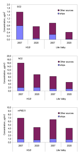
Figure 4.21 Development in the concentrations of SO2, NO2 and model calculated mPM2.5 at the urban background station at the H.C. Ørsteds Institute (HCØ) and at the rural background station Lille Valby.
[6] European Monitoring and Evaluation Programme. Full name: Co-operative Programme for Monitoring and Evaluation of the Long-Range Transmission of Air Pollutants in Europe.
5 Pollution from ships in ports
- 5.1 Introduction
- 5.2 Available studies
- 5.3 Sulphur regulation
- 5.4 Methodology: Emission inventories for ports
- 5.5 Results
- 5.6 Results for Copenhagen
- 5.7 Cruise ships and air quality
- 5.8 High rise buildings
- 5.9 Results: The Port of Aarhus
- 5.10 Conclusions concerning ships in port
5.1 Introduction
A minor component of the present project concerns the contribution to local air pollution from ships at port.
The model calculations in the previous chapters are performed with the DEHM model which has a spatial resolution of 6 x 6 km. In order address the question of the contribution to local air pollution from ships at port such resolution is inadequate. Therefore, a different methodology must be used. The present chapter presents an overview, based on previous studies as well as updated information on the current situation and on the expected developments. Information is provided for the ports of Copenhagen and Aarhus, with most details for Copenhagen.
One particular previous study is unmatched in its degree of detail, namely a study on cruise ships calling the port of Copenhagen (Olesen and Berkowicz, 1005). That study is used to infer several useful conclusions (mainly in Section 5.7).
The chapter contains the following parts:
- Section 5.2 gives on overview of available studies. The discussion of pollution from ships in ports utilizes methodology and results from previous studies.
- Section 5.3 gives an overview of sulphur regulation in ports, which is more stringent than for ships at sea.
- Section 5.4 explains the methodology used in compiling emission inventories for the ports of Copenhagen and Aarhus.
- Section 5.6 presents results concerning emissions for the Port of Copenhagen.
- Section 5.7 focuses on cruise ships. Cruise ships in Copenhagen contribute substantially to emissions in the port, and therefore a discussion on pollution from cruise ships is given.
- Section 5.8 briefly discusses high rise buildings close to ports, which has been an issue of interest in Copenhagen.
- Section 5.9 presents results concerning emissions in Aarhus.
- Section 5.10 summarises conclusions from the chapter.
5.2 Available studies
A frame of reference for many of the estimates made in the present chapter is a report by Oxbøl and Wismann (2003). It provides an inventory of emissions from ships in three Danish ports (Copenhagen, Køge and Helsingør), and also gives a crude estimate of emissions for ports in the entire country. The methodology used by Oxbøl and Wismann has been used here to produce updated estimates for the ports of Copenhagen and Aarhus.
A detailed study of the contribution to air pollution by cruise ships in the Port of Copenhagen was prepared by Olesen and Berkowicz (2005). Pollution with NO2 received particular attention in that study. As part of the study a detailed emission inventory of cruse ships calling at the Port of Copenhagen in 2004 was compiled by Force Technology; it is described in an appendix to the report by Olesen and Berkowicz. Based on this inventory, combined with data for the physical characteristics of the cruise ships, meteorology and background concentrations, the authors carried out atmospheric dispersion calculations for various pollutants. The Danish OML model was used for the computations. It was concluded that the increase of NO2 concentrations resulting from the presence of cruise ships was not capable of increasing the level of NO2 above the limit values, neither close to the ships nor far away from them. This conclusion concerns the contribution from cruise ships to the general pollution level; it does not preclude that there may be local violations of NO2 limit values in very busy streets due to the traffic load. The discussion is elaborated in Section 5.7, taking into account updated information, the new emission inventory, and also considering other pollutants that NO2.
A further study which provides background information for the present study is an environmental assessment of the air pollution level for a planned pair of high rise buildings at Marmormolen in Copenhagen (COWI, 2009). The buildings are close to several ferries in the port of Copenhagen, and the presence of nearby ferries could potentially constitute a problem for the air quality in the buildings. The environmental assessment shows that in this specific case there is no conflict with air quality limit values. However, the scenario of a high rise building close to a ship berth is a matter deserving consideration, and it is discussed in Section 5.8.
There are plans to establish a new cruise terminal at Nordhavn in Copenhagen. The environmental assessment for this project (Grontmij/Carl Bro, 2009) provides additional information that enters into the current study.
Besides the publications mentioned above, much additional information has been compiled through personal contacts with Copenhagen Malmö Port (Gert Nørgaard), Port of Aarhus (Søren Tikjøb), the Danish Petroleum Association (i.e. Energi- og Olieforum: Michael Mücke Jensen), Tom Wismann, Torm Shipping (Troels Jørgensen), MAN Diesel (Sven Henningsen), TR shipping (Anders Nødskov), Douglas Clark, Mols-Linien (Flemming Kristensen), Wärtsila (Johanna Vestergaard) and Royal Carribean International (Thomas Stjernhav).
5.3 Sulphur regulation
An important change which has occurred since many of the previous studies were completed, is that a set of requirements have been introduced, addressing sulphur in the fuel used when ships are at port. EU directive 2005/33/EC defines requirements to the maximum sulphur content of marine fuels used by ships at berth in Community ports. It prescribes that by 1 January 2010, a ship at berth is not allowed to use marine fuel with a sulphur content exceeding 0.1%. There are slight exemptions; thus, if a ship according to timetables is due to be at berth for less than two hours, it does not have to change fuel.
The regulations were implemented in Denmark by Statutory Order No. 1663 of 14 December 2006. For gas oil, a requirement of 0.1 % sulphur has applied already since January 2008.
The emission inventories presented in Section 5.6 and 5.9 are based on the regulations that will be in place in 2010: 0.1% sulphur content for ships at dock, and 1% sulphur content for manoeuvring, as required by the SECA regulations by March 2010.
5.4 Methodology: Emission inventories for ports
The emission inventory presented here is meant to provide an estimate of emission from ships in the ports of Copenhagen and Aarhus. The estimate does not claim to be accurate, but is prepared to the same level of detail as the previous investigation by Oxbøl and Wismann (2003). Basically, it applies the same methodology. However, there are some exceptions, where updated information makes a change pertinent.
Inventories of ships calling at the ports of Copenhagen and Aarhus in 2008 have been provided by the respective port authorities (personal communication: Gert Nørgaard, CMP and Søren Tikjøb, Port of Aarhus). The inventory for Copenhagen is the most detailed with information on when and where each ship called, while the information from Aarhus contains summarised information for classes of ships.
The methodology in Oxbøl and Wismann (2003) has been used. This represents a simplified approach compared to the one followed in Chapter 2 on emissions from ships at sea. Thus, ships have been classified according to the following categories:
- Tankers
- Bulk carriers (including various special ships)
- Container ships
- Ro-Ro ships
- Passenger ferries
- Cruise ships
5.4.1 Activities: At dock, pumping and manoeuvring
Estimates of energy consumption have been based on the same principles and assumptions as Oxbøl and Wismann (2003) with a few exceptions. Oxbøl and Wismann consider emissions caused by the following activities:
- Manoeuvring (arrival and departure at the dock)
- Activities at dock (generating of electricity)
- For tankers only: oil pumping
A set of assumptions provides a link from the size of ships in gross tonnage to the size of the main and auxiliary engines, and further – considering the load of engines and the duration of the various activities – to an energy consumption for each activity and ship class.
Table 5.1 lists the assumptions that are used here. The table is based on table 3.3 in Oxbøl and Wismann (2003). There are a few differences, however.
Concerning cruise ships at dock, the detailed study by Olesen and Berkowicz (2005) provides a relationship between size and power consumption at dock, based on responses to a questionnaire to ship owners. This relationship is indicated in Table 5.1.
Concerning pumping, the report by Oxbøl and Wismann (2003) assumed the pumping of 1 ton oil would require 0.7 kg fuel. This value was quoted from a single reference in literature, but Oxbøl and Wismann were not able to verify it.
The present estimate is based on information from the Danish Petroleum Association (pers. communication Michael Mücke Jensen) and from TORM Shipping (Troels Jørgensen). Ship-based pumps, driven by auxiliary engines, are used for unloading oil. For loading, land-based pumps driven by ordinary power supply are used. On ships, different types of machinery are used for pumping, and the energy consumption depends on local conditions at the port (the pumping distance, the height to which the oil should be pumped etc.). However, in the Port of Copenhagen pumping does not require much energy. The estimate from the Danish Petroleum Association is that pumping of 1000 m³ oil per hour requires a power supply of 50-60 kW. This value has been used for the calculations here, and is indicated in the table. It leads to substantially lower estimates for power consumption for pumping than the estimate by Oxbøl and Wismann.
The assumed duration of the various activities is indicated in Table 5.1. The energy consumption for dock and manoeuvring is computed as the product of the power, the engine load and an estimated duration of the activity. The estimated times is indicated in the table. For manoeuvring it follows Oxbøl and Wismann (2003). For time at dock the values are based on the ship list for Copenhagen 2008. Tankers are at port on average 11.2 hours, container ships 11.7, cruise ships 12.5, while the group labelled 'bulk carriers' is assumed to be at dock for 19 hours; the latter group is mixed and includes various types of special ships. The average of 19 hours is based on bulk carriers. An exception is made for the RoRo ferry Tor Corona in Copenhagen, for which more detailed information is available from COWI (2009).
Concerning ferries, in the port of Copenhagen information is taken from the environmental assessment for Marmormolen by COWI (2009). It contains detailed information on emissions for the ferries to Oslo (Crown of Scandinavia and Pearl of Scandinavia), the ferry to Poland (Pomerania) and for the Ro-Ro freight line to Klaipeda (Tor Corona). Where available, this detailed information has replaced the general rough estimates.
For the port of Aarhus, information on emission for ferries is from Mols-Linien (personal communication, Flemming Kristensen).
Table 5.1 Overview of assumptions and calculation procedures
| Ship type | Activity | Parameter | Assumption/procedure The indicated times at dock are for Copenhagen - Table 5.4 gives values for Aarhus. |
| Tankers | At dock | Auxiliary engine | Engine used for 11.2 hours with power consumption: Paux = 0.0185 * PME + 183.14 (kW) where PME is main engine size |
| Manoeuvring | Main engine | Used for 0.5 hours at 25 % load. PME = 0.5105 * GT + 465.56 (kW) where GT is tonnage. |
|
| Pumping | Energy consumption | 0.071 kWh per ton unloaded oil | |
Bulk carriers etc |
At dock and manoeuvring | As for tankers, but 19 hours at dock | |
Container ships |
At dock and manoeuvring | As for tankers, but 11.7 hours at dock and main engine size PME = 0.709 * GT + 420.84 (kW) |
|
Ro-Ro |
At dock and manoeuvring | Auxiliary engine as for tankers, but main engine size PME = 0.7053 * GT + 776.33(kW) |
|
Ferries |
At dock | Detailed information for each ferry is available. | |
| Manoeuvring | Used for 0.5 hours at 50 % load. Engine size known for each ferry. | ||
Cruise ships |
At dock | Auxiliary engine | 12.5 hours at dock with power consumption Paux = 0.084 * GT + 242.58 (kW) |
| Manoeuvring | Main engine | Used for 0.5 hours at 25 % load. Average estimated PME = 30000 kW (based on known values for some of the cruise ships). |
5.4.2 Emission factors
In general, the emission factors listed in Table 5.2 have been used. However, for ferries, more detailed information is available and forms the basis for the computations. A few comments on the emission factors in Table 5.2 are appropriate.
Table 5.2 Emission factors used in the inventory for ships in port.
| Main engine (g/kWh) |
Auxiliary engine (g/kWh) |
|
| NOX | 12 | 11 |
| SO2 | 4.0 | 0.4 |
| PM (total) | 0.36 | 0.18 |
| CO | 1.6 | 1.6 |
| VOC | 0.5 | 0.5 |
| Assumed sulphur content | 1 % | 0.1 % |
For NOX, the emission factors are those applied by Oxbøl and Wismann (2003). The more detailed approach that is applied in Chapter 2 of the present report is not used, because the ship data are not sufficiently detailed. It should be mentioned that use of the NOX emission factor from the table will result in a substantial overestimate of NOX emissions from gas turbines (around a factor of three). Gas turbines are used as auxiliary engines for some ships – e.g., some cruise ships.
Concerning the ferries, more accurate estimates for NOX emission factors than those shown in the table are used. This makes a large difference for the Oslo ferries, which use SCR (selective catalytic reduction) technology to reduce NOX emissions, and for the ferries Mai Mols and Mie Mols, which are equipped with gas turbines.
For SO2 an emission factor based on expression (8) in Chapter 2 is used. Further, for the results shown in the subsequent sections, a sulphur content has been assumed of, respectively, 0.1 for ships at dock and 1.0 % for manoeuvring. This corresponds to the situation in 2010 after the strengthening of the SECA requirements. It is lower than that used by Oxbøl and Wismann (2003).
The particle emission factors in Table 5.2 are based on equation (10) in Chapter 2.
It should be noted that all computations use emission factors for ship engines meant to represent conditions averaged over time. When engines are started there may be a burst of pollution, which is not accounted for. To the extent that such emissions take place, they may be a cause of nuisance, although they don't have much influence on average conditions.
5.5 Results
Based on the assumptions indicated in the previous sections, inventories have been compiled for Copenhagen and Aarhus. They will be discussed in the subsequent sections. The discussion for Copenhagen is most exhaustive, and it is supplemented by discussions on cruise ships and high rise buildings.
5.6 Results for Copenhagen
In the case of Copenhagen, two previous inventories exist that can be used for comparison and reference:
- The one by Oxbøl and Wismann (2003) which is based on traffic data for 2001. In the subsequent graphs these results are labelled '2001'.
- The one focusing exclusively on cruise ships which was compiled by Force Technology and used by Olesen and Berkowicz (2005). It uses traffic data from 2004. In the following figures it is referred to as '2004'.
Table 5.3 Port of Copenhagen. Energy consumption and emission of various components in 2008. These values are displayed en Figure 5.1 and Figure 5.2.
| Activity at dock | Manoeuvring | ||||||||
| No. of calls | Energy cons. (MWh) | NOx (t) |
SO2 (t) |
PM (t) |
Energy cons. (MWh) | NOx (t) | SO2 (t) | PM (t) |
|
| Tankers | 1021 | 2857 | 31 | 1.1 | 0.5 | 319 | 3.8 | 1.3 | 0.1 |
| Other bulk carriers | 1212 | 4860 | 53 | 1.9 | 0.9 | 518 | 6.2 | 2.1 | 0.2 |
| Container ships | 493 | 1642 | 18 | 0.7 | 0.3 | 338 | 4.1 | 1.4 | 0.1 |
| Ferries | 586 | 6398 | 21 | 3.7 | 1.7 | 2908 | 34.9 | 11.6 | 1.0 |
| Cruise liners | 297 | 16974 | 187 | 6.8 | 3.1 | 1114 | 13.4 | 4.5 | 0.4 |
| Total | 3609 | 32730 | 310 | 14.2 | 6.6 | 5197 | 62.4 | 20.8 | 1.9 |
The current, updated, estimate is labelled '2010', because it represents the situation in 2010 concerning sulphur content in fuel (although it is based on traffic data from 2008). The results of the inventory are tabulated in Table 5.3.
Figure 5.1 shows a key parameter for the inventory: Energy consumption during a year. The left panel of the figure shows values referring to activities at dock ("docking"), including pumping. Ro-Ro ships were not treated separately for Copenhagen in Oxbøl and Wismann (2003); these ships are therefore also here included among "Other bulk ships".
The right panel shows energy consumption during manoeuvring, based on the assumption that a total time of 0.5 hours is required to enter and leave the port.
Some noticeable features stand out from the left panel ('Docking'). For tankers, there is a considerable decrease from '2001' to '2010'. This is due to the previous assumption that pumping from tankers is very energy consuming – an assumption which is not in agreement with recent information from the Danish Petroleum Association.
There is a notable decrease in energy consumption for ferries. There are now only two passenger ferry lines in Copenhagen: to Oslo and to Poland. In 2001, there was also a line for Bornholm.
For bulk ships and container ships there are differences which reflect the combined effect of a different number of ships, their size distribution, and the time spent at dock, which is used for energy consumption computation. The duration was previously estimated as 8.8 hours for tankers, bulk ships and container ships. This was based on data from one month. According to the list of ships from 2008, the duration is longer than 8.8 hours (see Table 5.1). In computing the average duration of a stay, outliers have been removed, due to the assumption that a ship does not use its auxiliary engine all of the time during a very long stay. It must be recognized that for these ship types the methodology is suitable to provide an overview, but that the accuracy can be questioned. When comparing the left and right panel, it appears that energy consumption during docking dominates over energy consumption during manoeuvring.
The number of cruise ships calling at Copenhagen has increased gradually: From 201 calls in 2001 to 259 in 2004, and further to 295 in 2008. Accordingly, there is an increase in energy consumption for cruise ships.
Figure 5.2 shows the situation for emission of the pollutants NOX, SO2 and PM. The figure for NOX reflects the same pattern as the graph for energy consumption. Note that for cruise liners a column has been added, referring to the study based on 2004 data. The total NOX emission for ships was 523 t in 2001, and has decreased to 373 t for the 2010 inventory. The reduction is caused partly by the change of the assumption concerning pumping, and partly because the contribution from ferries has decreased even more than the decrease in energy consumption justify. The reason is the use of SCR technology on the Oslo ferries, which reduces their NOX emissions by around 85 percent.
For reference, the emission of NOX from ship activity can be compared to other large NOX sources:
- The sum of NOX emissions from ships is estimated at 373 t in 2010;
- Cruise ships are responsible for 200 t of these;
- The power plant Amagerværket 568 t emitted in 2008;
- Emission by ships in Øresund according to Chapter 3: 7760 t in 2007;
- Emissions by all road traffic in the region of Copenhagen: 19000 t.
In Figure 5.2, the graph for SO2 at dock for cruise ships displays an awkward development with very low values for the 2001 inventory, a much higher value in 2004, and a moderate value for 2010. The reason is an unrealistic assumption in the 2001 inventory: It was assumed that cruise ships used fuel with a sulphur content as low as 0.05 percent. The study in 2005 involved use of a questionnaire to the shipping companies, and it was revealed that the actual sulphur content used by cruise ships while at berth in Copenhagen ranged from 0.2 to 3.2% with a mean around 1.6%. In 2010 the maximum allowed sulphur content while at quay is 0.1 %; this reduces sulphur emission by a factor of 16 compared to the 2004 case.
For PM (primary particles, all sizes), the total decreases from 13 to 8 t. Particle emission depends somewhat on sulphur content in the fuel, so a decrease is to be expected. The largest single contribution to the decrease is, however, correction of the assumptions concerning pumping.
The distribution of NOx emission by district is shown in Figure 5.3. The figure includes activities at dock and pumping, but not manoeuvring. It is appears from the figure that Frihavnen has the largest load. Of the 145 t NOX emitted in Frihavnen, 88 are due to cruise ships.
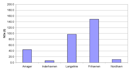
Figure 5.3 Distribution of NOx emission in various districts in the Port of Copenhagen.
5.7 Cruise ships and air quality
According to the inventory, cruise liners are responsible for a substantial part of NOX emission - 200 t compared to the total of 373 t (including all activities). The present section focuses on cruise ships.
It is interesting to examine how the emission load for cruise ships is distributed geographically. Figure 5.4 shows the NOX emission load according to the study using 2004 data, as well as the new inventory.
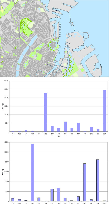
Figure 5.4 Geographical distribution of NOx emission load from cruise ships at berth in 2004 (top) and 2008 (bottom).
In 2008, cruise ship emission predominantly took place at three berths: no. 192 at Langelinie, and no. 245 and 254 in Frihavnen. However, the situation with a heavy emission load at these berths is not permanent, because there are plans to establish a new cruise terminal from 2012 North of the present, as indicated in Figure 5.5.
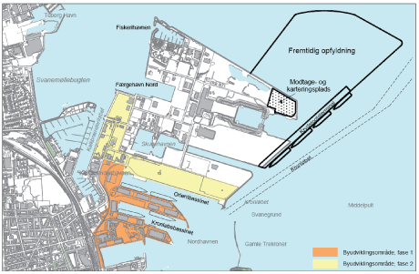
Figure 5.5 Plans for new terminal for cruise ships.
Carl Bro/Grontmij (2009) has carried out an environmental assessment in preparation to the construction of the new terminal. The assessment report does not include any details on the influence of cruise ships on the air quality after the establishment of the terminal, but notes that the issue is one of an existing pollution source that is moved. Further, the report indicates that there are plans to establish land-based power supply, which can be put to use in a long term perspective.
Within the present study we have not carried out atmospheric dispersion calculations, because a new estimate that matches the previous study by Olesen and Berkowicz (2005) in degree of detail is outside the scope of the current work. Also, Olesen and Berkowicz (2005) provide sufficient evidence to draw useful conclusions.
In the next section we will recapitulate some important conclusions from the previous report, while adding new information.
5.7.1 Cruise ships: NOX
The exhaust gas from combustion engines – such as the engines in cruise ships – contains a mixture of nitrogen oxides (NOX). NOX is the sum of NO and NO2. In terms of health effects and limit values, NO2 is the substance of interest. When emitted from a ship engine, NO is much more abundant than NO2. Only 5-10% is emitted directly as NO2. NO can be gradually converted to NO2 by reactions in the atmosphere. Fast conversion is possible if ozone is available.
When evaluating concentrations of NO2 it is important to be aware that there is not a one-to-one correspondence between NOX and NO2; close to sources of pollution, concentrations of NOX can be much higher than those of NO2.
It is also important to note that the amount of available ozone in the background air sets a "ceiling", which limits the amount of NO that can be converted to NO2. The concept of a "ceiling" set by ozone applies to dispersion at a local scale, not to long-range transport. Thus, if we consider the effect that cruise ships have on the level of NO2 pollution in Copenhagen, the mechanism of limiting by ozone is important. Accordingly, the emission of NOX from cruise ships is reflected by only a small increase in NO2 concentrations in the streets of Copenhagen. The calculations that were carried out in the detailed study by Olesen and Berkowicz (2005) used the Danish OML model in 'chemistry mode', which takes account of the ozone limiting mechanism.
For NO2, there are some parameters of key interest, because they refer to the EU directive on air quality from 2008 (2008/50/EC). The directive sets a limit for NO2 which is based on hourly concentrations. The hourly concentration of NO2 is allowed to exceed a limit of 200 μg/m³ no more than 18 times a year (this limit must be complied with in 2010).
Another limit value for NO2 refers to the annual average, which must not exceed 40 μg/m³ (from 2010).
In the 2005 study, the OML dispersion model was run several times, based on various sets of assumptions, e.g. concerning the base year for meteorology, for background concentrations etc. The so-called Basic Run is representative for the results.
Some main results from the Basic Run are presented in Figure 5.6. These results can be compared to the first limit value mentioned above. The map shows the 19th highest NO2 concentration during one year concentrations, resulting from the combined effect of cruise ships and the urban background pollution in the city of Copenhagen. The background pollution is assumed constant throughout the area. The values in Figure 5.6 are all in the interval between 98 and 101 μg/m³; according to the directive they are required to be less than 200 μg/m³. If the cruise ships had not been present, Figure 5.6 would have shown a constant value of 98 μg/m³, corresponding to the contribution from the urban background pollution.
The results presented above are meant to illustrate the contribution to NO2 concentration level, by comparing a reference situation where there is only background pollution with a situation where cruise ships have been superimposed on this reference situation. It is clear from the results that the 19th highest NO2 concentration value is not increased much by the presence of the cruise ships. In a busy street, NO2 concentration levels will be higher, and here the contribution from cruise ships will be even less able to affect the 19th highest concentration than in the situation depicted in Figure 5.6.
In the study by Olesen and Berkowicz (2005), the conclusion as to NO2 average concentrations was that concerning the annual average concentration of NO2, the Basic Run results in a level of around 23 μg/m³, almost unaffected by the presence of cruise ships. Their maximum contribution is 0.8 μg/m³ at the location where the impact is greatest (600 m east of Langelinie, in the Øresund). These numbers should be compared to a limit value of 40 μg/m³
NOX emissions are 29% higher for cruise ships in the '2010' situation (based on traffic data from 2008) than they were according to the inventory based on 2004 data. A new set of detailed calculations must thus be expected to lead to slightly increased values compared to the previous study. If all other factors were equal, NO2 concentrations would be increased, but with substantially less than 29%, because of the limiting effect of ozone. As noted before, a study as detailed as Olesen and Berkowicz (2005) is outside the scope of the present work.
There is one assumption which might be changed if a new, detailed study were conducted. To some extent gas turbines are used by cruise ships while at berth, whereas the emission factor for NOX that was used for the computations is representative of diesel engines. Compared to a diesel engine, a gas turbine emits only around one third of the NOX amount per kWh. With a detailed inventory the emitted NOX amount would be smaller than assumed here.
Further it can be noted that some issues which were questioned during the previous study have been clarified. In the previous study, four sets of assumptions concerning the fraction of directly emitted NO2 were used. The exhaust gas from combustion is a mixture of NO and NO2. The 'Basic Run' was conducted under the assumption that 10% of NOX is emitted directly as NO2. It has been confirmed that this is reasonable as an upper estimate. MAN Diesel (personal communication, Svend Henningsen) indicates that the percentage of directly emitted NO2 is 5-10%, and closer to 5 than 10.
The previous study assumed that SCR (selective catalytic reduction) technology for reduction of NOX emissions was not applied by cruise ships. Recent information confirms that this assumption is reasonable for the time being. However, it will change, especially after 2016.
In year 2011 the IMO Tier II NOX standard will enter into force. This means that all new installations have to meet a 20% reduced NOX emission level compared to now. The 20% NOX reduction can be achieved by engine internal methods. No exhaust gas after-treatment system will be needed (pers. communication from Johanna Vestergaard, Wärtsilä).
However, in 2016 the IMO Tier III NOX standard will enter into force in the so-called NECA areas. The Danish Marine waters are expected to be appointed NECA's. In these areas an 80% NOX reduction from today’s Tier I level will be required for new ships. For achieving an 80% NOX reduction, an SCR exhaust gas after-treatment system is a likely option.
5.7.2 Cruise ships: particles and SO2
Besides NOX pollution, the previous study by Olesen and Berkowicz (2005) considered pollution with SO2 and particles. It was found that the largest increase in particle pollution level (primary particles on an annual basis) was 0.035 μg/m³. This can be compared to the forthcoming annual limit value of 25 μg/m³ for PM2.5, and to the levels indicated in Chapter 5.
For SO2, the contribution in the most exposed area (in the water West of Langelinie) was 1.5 μg/m³ in 2004. The SO2 contribution from the previous study will be reduced by a factor 16 after 2010 when the regulations concerning sulphur content in fuel for ships at port come into effect.
5.8 High rise buildings
The study by Olesen and Berkowicz (2005) considered pollution levels mainly at a height of 1.5 meters, but with some additional calculations for a height of 7 meters. For the current study, some additional calculations have been carried out based on the data for the 2005 study, but for greater heights than 1.5 and 7 meters. They show that a height of around 50 meters is most critical in respect to compliance with the NO2 limit value, and that at this height there may be problems with compliance within a distance of around 100 m from the ships.
When planning high rise buildings close to berths, it is recommended to conduct studies of sufficient detail to verify whether there is a potential problem.
A study by COWI (2009) presents such computations for the case of a two planned buildings at Marmormolen that are situated close to the Oslo ferry. These ferries are equipped with SCR gas cleaning technology, and it is demonstrated that the ferries are no cause of concern in respect to NO2 levels.
5.9 Results: The Port of Aarhus
The Port of Aarhus is Denmark's largest container port and public bulk terminal. Figure 5.7 is a map of the Port of Aarhus. It indicates the current positions where the various types of ships pertain, and also plans for future developments (the map should be considered a draft only).
For the port of Aarhus, an emission inventory similar to the one for Copenhagen has been prepared. It is based on summarised information on ship traffic received from Søren Tikjøb (Port of Aarhus) as well as information on the ferries of Mols-Linien (Flemming Kristensen). Key information is listed in Table 5.4.
The information for Aarhus concerning the duration of stay differs somewhat from that of Copenhagen. In particular, one may note the long duration of stay for bulk carriers (48 hours as opposed to 19 hours for Copenhagen). As to manoeuvring, the same assumptions as for Copenhagen are used in general (a duration of 0.5 hour per call). For ferries, the duration is shorter with a lighter load (5 minutes, 15% load, according to information from Mols-Linien.).
Table 5.4 Key information on ship traffic to the port of Aarhus
| Type | Number | GT sum (mio) | GT average | Duration of stay (hours) |
| Tankers | 548 | 1.857 | 3389 | 15 |
| Bulk carriers | 903 | 3.607 | 3994 | 48 |
| Container ships | 964 | 14.147 | 14675 | 18 |
| Ro-Ro | 213 | 2.728 | 12808 | 12 |
| Cruise liners | 21 | 1.006 | 47905 | 8 |
| Sum excl. ferries | 2649 | 23 |
Figure 5.8 presents results for emissions at the Port of Aarhus. The underlying numbers are tabulated in Table 5.5.
As Aarhus is Denmark's largest container port and public bulk terminal, the energy consumption and emission connected with bulk carriers and container ships are larger than those of Copenhagen (the duration of stay also plays a role, but is also stipulated as being longer for Aarhus).
The emission loads are somewhat smaller than those of Copenhagen. Figure 5.9 gives a comparison of various totals for the two ports. The energy consumption, NOX emission load, etc. are compared in a relative sense. All emission loads are smaller for Aarhus than for Copenhagen, and amount to 45-75% of the Copenhagen values.
Table 5.5 Port of Aarhus. Energy consumption and emission of various components in 2008. Corresponds to Figure 5.8.
| Activity at dock | Manoeuvring | ||||||||
| No. of calls | Energy cons. (MWh) | NOx (t) |
SO2 (t) |
PM (t) |
Energy cons. (MWh) | NOx (t) | SO2 (t) | PM (t) |
|
| Tankers | 548 | 1925 | 21 | 0.8 | 0.4 | 150 | 2 | 0.6 | 0.1 |
| Other bulk carriers | 903 | 9946 | 109 | 4.0 | 1.8 | 283 | 3 | 1.1 | 0.1 |
| Container ships | 964 | 6653 | 73 | 2.7 | 1.2 | 1304 | 16 | 5.2 | 0.5 |
| Ro-Ro | 213 | 932 | 10 | 0.4 | 0.2 | 261 | 3 | 1.0 | 0.1 |
| Ferries | 4590 | 1464 | 15 | 1.2 | 0.3 | 1223 | 7 | 1 | 0 |
| Cruise liners | 21 | 717 | 8 | 0.3 | 0.1 | 79 | 1 | 0.3 | 0.0 |
| Total | 7239 | 21637 | 237 | 9.2 | 4.0 | 3301 | 32 | 9.3 | 1.0 |
Figure 5.9 Comparison of various totals for Aarhus relative to Copenhagen.
5.10 Conclusions concerning ships in port
The following conclusions can be inferred from previous studies on concentration levels, combined with updated emission information:
- Cruise ships are a considerable source of NOX pollution in Copenhagen. Cruise ships are responsible for around 55% of NOX emissions from ships at port in Copenhagen. The NOX emission from cruise ships is estimated to be 30% larger in 2008 than it was in a previous, detailed study referring to 2004. In Aarhus, cruise ships are only responsible for around 3% of NOX emissions.
- It is important to note that there is not a one-to-one correspondence between NOX and NO2. For instance, a 30% increase of NOX emissions will lead to an increase of concentration levels of NO2 which are smaller than 30% when we consider local scale (such as Copenhagen).
- The local NO2 levels, at ground close to cruise ships (within the nearest 500 m or so) are well below EU limit values - unless cases can be found where heavy car traffic bring the NO2 concentrations at such locations to a critical level. Thus, on an annual basis the increase of NO2 concentrations due to cruise ships was found in the 2004 study to be 0.8 μg/m³ at the location where the impact was greatest (600 m from the ships, in the Øresund). This should be seen in the context of an urban background level on the order of 20 μg/m³ and a limit value of 40 μg/m³.
- When considering conditions at high rise buildings close to berths with very heavy ship traffic, there may potentially be problems with NO2 exceedances very close to the berth (within the nearest hundred or few hundred meters). In such cases it can be wise to conduct detailed studies. As an example, it has been demonstrated that for planned high rise buildings (ca. 100 m tall ) at Marmormolen in Copenhagen located approximately 250 m from the berth of the Oslo ferries the presence of the Oslo ferries will not lead to violations of the NO2 limit values.
- The increase in yearly averaged concentration levels for primary particles due to the presence of cruise ships at quay in Copenhagen was found in the 2005 study to be small: 0.035 μg/m³at the most critical location 200 m from the ships. This can be seen in the context of the limit value of 25 μg/m³ for PM2.5 and the contribution of all ships in general, which is slightly less than 1 μg/m³ according to section 4.9. It should be noted, however, that this estimate is based on emission factors representing time-averaged values for engines in ordinary operation. When engines change operating conditions there may be bursts of smoke which are not accounted for in the present estimates, but may be a cause of nuisance.
- For the port of Aarhus, the total energy consumption and the total of emissions for all substances is smaller than it is for Copenhagen. However, for certain ship types (container ship, other bulk carriers) the load at the port of Aarhus is larger than for Copenhagen.
6 Conclusions
Conclusions are summarised in the chapter Summary and conclusions in front of the report.
7 References
Amann, M., Bertok, I., Cofala, J., Heyes, C., Klimont, Z., Rafaj, P., Schöpp, W., Wagner, F. (2008). National Emission Ceilings for 2020 based on the 2008 Climate & Energy Package. NEC Scenario Analysis Report Nr. 6. International Institute for Applied Systems Analysis (IIASA). Laxenburg, Austria.
Bach, H., Andersen, M.S., Illerup, J.B., Møller, F., Birr-Pedersen, K., Brandt, J., Ellermann, T., Frohn, L.M., Hansen, K.M., Palmgren, F., Nielsen, J.S. & Winther, M. (2006): Vurdering af de samfundsøkonomiske konsekvenser af Kommissionens temastrategi for luftforurening, Danmarks Miljøundersøgelser, Aarhus Universitet. Faglig rapport fra DMU nr. 586 90 s. Tilgængelig på: http://person.au.dk/da/pub/12551981
Cofala, J., Amann, M., Heyes, C., Wagner, F., Klimont, Z., Posch, M., Schöpp, W., Tarrasón, L., Jonson, J., Whall, C. and Stavraki, A. (2007): Analysis of Policy Measures to Reduce Ship Emissions in the Context of the Revision of the National Emissions Ceiling Directive, Final Report, IIASA Contract No 06-107, April 2007.
Corbett, J.J., & H.W. Köhler 2003: Updated emissions from ocean shipping, Journal of Geophysical Research, 108, D20, 4650, doi:10.1029/2003JD003751.
COWI (2009): Marmolen P/S. Vurdering af eksisterende luftkvalitet.
DTU (2009): Unpublished data material provided by Senior researcher Hans Otto Kristensen, Department of mechanical engineering, Section of coastal, maritime and structural engineering, DTU.
Ellermann, T., Andersen, H.V., Bossi, R., Christensen, J., Geels, C., Kemp, K.., Løfstrøm, P., Mogensen, B.B. & Monies, C. (2009): Atmosfærisk deposition 2007. NOVANA. Danmarks Miljøundersøgelser, Aarhus Universitet. 97 s. Faglig rapport fra DMU, nr. 708. http://www2.dmu.dk/Pub/FR708.pdf
EMEP (2008): www.ceip.at Web site of EMEP Centre on Emission Inventories and Projections (CEIP).
EMEP/CORINAIR, 2009: EMEP/EEA air pollutant emission inventory guidebook — 2009, prepared by the UNECE/EMEP Task Force on Emissions Inventories and Projections, Technical report/2009. Available at http://www.eea.europa.eu/publications/emep-eea-emission-inventory-guidebook-2009 (14-09-2009).
Endresen, Ø., E. Sørgård , J.K. Sundet, S.B. Dalsøren, I.S.A. Isaksen, T.F. Berglen, and G. Gravir 2003: Emission from international sea transportation and environmental impact, Journal of Geophysical Research. 108, D17, 4560, doi:10.1029/2002JD002898.
Entec (2005a), European Commission Directorate General Environment Service Contract on Ship Emissions: Assignment, Abatement and Market-based Instruments. Task 1 - 64, Preliminary Assignment of Ship Emissions to European Countries. Final Report Entec UK Limited, August 2005.
Entec (2005b), European Commission Service Contract on Ship Emissions: Assignment, Abatement and Market-based Instruments. Task 2 – General Report, Final Report, Entec UK Limited, August 2005.
Entec (2005c), European Commission Service Contract on Ship Emissions: Assignment, Abatement and Market-based Instruments. Task 2b – NOx Abatement, Final Report, Entec UK Limited, August 2005.
Entec (2005d), European Commission Service Contract on Ship Emissions: Assignment, Abatement and Market-based Instruments. Task 2c – SO2 Abatement, Final Report, Entec UK Limited, August 2005
Eyring, V., H.W. Köhler, J. van Aardenne, and A. Lauer 2005: Emissions from international shipping: 1. The last 50 years, Journal of Geophysical Research., 110, D17305, doi:10.1029/2004JD005619.
Georgakaki, A., Coffey, R.A., Lock, G., Sorenson, S.C. (2005): Transport and Environment Database System (TRENDS): Maritime air pollutant emission modelling. Atmospheric Environment 39 (2005) 2357-2365.
Grell, G. A., Dudhia, J. and Stauffer, D. R. (1995): A description of the fifth-generation Penn State/NCAR Mesoscale Model (MM5), Mesocale and Microscale Meteorology Division, National Centre for Atmospheric Research, Boulder, Colorado, NCAR Technical Note, NCAR/TN-398+STR, pp. 114
Grontmij/Carl Bro (2009): Udvidelse af Københavns Nordhavn og ny krydstogtterminal. VVM. Teknisk baggrundsrapport nr. 9. Luftforurening og klima. Marts 2009.
Hertel, O., Ambelas Skjøth, C., Frohn, L. M., Vignati, E., Frydendall, J., de
Leeuw, G., Swarz, S., and Reis, S., 2002: Assessment of the Atmospheric Nitrogen and sulphur Inputs into the North Sea using a Lagrangian model. Phys. Chem. Earth, 27(35), 1507-1515.
IMO MEPC (2009): Interim guidelines on the method of calculation of the energy efficiency design index for new ships, Ref. T5/1.01, MEPC.1/Circ.681, 17 August 2009.
Kemp, K., Ellermann, T., Brandt, J., Christensen, J., Ketzel, M. & Jensen, S.S., 2008: The Danish Air Quality Monitoring Programme. Annual Summary for 2007. National Environmental Research Institute, University of Aarhus. 47 pp. NERI Technical Report No. 681. http://www2.dmu.dk/Pub/FR681.pdf
Lloyd’s Register of Shipping 1995: Marine Exhaust Emissions Research Programme. Lloyd’s Register Engineering Services, United Kingdom, London.
Ministry of Transport 2000: TEMA2000 - et værktøj til at beregne transporters energiforbrug og emissioner i Danmark (TEMA2000 - a calculation tool for transport related fuel use and emissions in Denmark). Technical report. Available at http://www.trm.dk/sw664.asp
Nielsen, O-K., Winther, M., Mikkelsen, M.H., Hoffmann, L., Nielsen, M., Gyldenkærne, S., Fauser, P., Jensen, M.T., Plejdrup, M.S. & Illerup, J.B. 2008: Annual Danish Emission Inventory Report to UNECE. Inventories from the base year of the protocols to year 2006. National Environmental Research Institute, University of Aarhus . 504 pp. – NERI Technical Report No. 675.
Olesen, H.R., Ellermann, T., Christensen, J. (2008): Luftforurening fra skibe - hvor stort er problemet? Presentation at the meeting Ren luft til alle, Copenhagen, December 3, 2008. http://ida.dk/netvaerk/idaforum/U0615a/Documents/Præsentationer%20efterår%202008/2008-12-02%20Ren%20Luft%20til%20alle%20præsentationer/Helge%20Rørdam%20Olesen.pdf
Olesen, H. and Berkowicz, R. (2005): Vurdering af krydstogtskibes bidrag til luftforurening. Miljøstyrelsen. - Miljøprojekt 978: 92 s.
Oxbøl, A. and Wismann, T.: Emissioner fra skibe i havn. Revideret udgave 2003. Arbejdsrapport fra Miljøstyrelsen Nr 49, 2003.
Penn State/NCAR Mesoscale Model (MM5). Mesoscale and Microscale Meteorology Division, National Centre for Atmospheric Research, Boulder, Colorado, USA. NCAR Technical Note, NCAR/TN-398+STR, pp. 114.
Wang, C., J.J. Corbett, and J. Firestone, Improving Spatial Representation of Global Ship Emissions Inventories, Environmental Science & Technology, Web Release Date: 01-Dec-2007;(Article) DOI: 10.1021/es0700799, 2007
Whall, C., Cooper, D., Archer, K., Twigger, L., Thurston, N., Ockwell, D., McIntyre and Ritchie, A. (2002), Quantification of emissions from ships associated with ship movements between ports in the European Community. Final Report. Entec UK Limited.
Winther (2008): Fuel consumption and emissions from navigation in Denmark from 1990-2005 - and projections from 2006-2030. Technical Report from NERI no. 650. 109 pp. Available at: http://www2.dmu.dk/Pub/FR650.pdf
Wismann, T. (2001): Energiforbrug og emissioner fra skibe i farvandene omkring Danmark 1995/1996 og 1999/2000 (Fuel consumption and emissions from ships in Danish coastal waters 1995/1996 and 1999/2000). The Danish Environmental Protection Agency. - Environmental Project 597.
Yttri, K.E., Aas, W., Tørseth, K., Stebel, K., Tsyro, S., Simpson, D., Merckova, K., Wankmüller, R., Klimont, Z., Bergström, R., van der Gon, H. D., Holzer-Popp, T. & Schroedter-Homscheidt, M. (2009): Transboundary particulate matter in Europe, Status report 2009. Joint CCC, MSC-W, CEIP and CIAM Report 2009. EMEP report 4/2009. 95 pp.
Annex A: Ship categories
Click here to see: Annex A Ship categories
Annex B: NOX emission factors for 2007, 2011 and 2020 for ship category/engine type combinations
| Year | Ship type (DTU) | Ship type (NERI) | Main engine type | Retrofit | NOx (g/kWh) |
| 2007 | Bulk carrier | Bulk carrier | High speed (4-stroke) | No | 11.170 |
| 2007 | Bulk carrier | Bulk carrier | Medium speed (4-stroke) | No | 11.673 |
| 2007 | Bulk carrier | Bulk carrier | Slow speed (2-stroke) | No | 17.827 |
| 2007 | Cargo Ro-Ro | Cargo Ro-Ro | High speed (4-stroke) | No | 11.170 |
| 2007 | Cargo Ro-Ro | Cargo Ro-Ro | Medium speed (4-stroke) | No | 11.673 |
| 2007 | Cargo Ro-Ro | Cargo Ro-Ro | Slow speed (2-stroke) | No | 17.827 |
| 2007 | Container | Container | High speed (4-stroke) | No | 11.170 |
| 2007 | Container | Container | Medium speed (4-stroke) | No | 11.673 |
| 2007 | Container | Container | Slow speed (2-stroke) | No | 17.827 |
| 2007 | Passenger Ro-Ro | Passenger Ro-Ro | Gas turbine | No | 4.000 |
| 2007 | Passenger Ro-Ro | Fishing | High speed (4-stroke) | No | 11.170 |
| 2007 | Passenger Ro-Ro | Other | High speed (4-stroke) | No | 11.170 |
| 2007 | Passenger Ro-Ro | Passenger Ro-Ro | High speed (4-stroke) | No | 11.170 |
| 2007 | Passenger Ro-Ro | Fishing | Medium speed (4-stroke) | No | 12.129 |
| 2007 | Passenger Ro-Ro | Other | Medium speed (4-stroke) | No | 11.673 |
| 2007 | Passenger Ro-Ro | Passenger Ro-Ro | Medium speed (4-stroke) | No | 11.673 |
| 2007 | Passenger Ro-Ro | Fishing | Slow speed (2-stroke) | No | 17.827 |
| 2007 | Passenger Ro-Ro | Other | Slow speed (2-stroke) | No | 17.827 |
| 2007 | Passenger Ro-Ro | Passenger Ro-Ro | Slow speed (2-stroke) | No | 17.827 |
| 2007 | Tanker | Tanker | Gas turbine | No | 4.000 |
| 2007 | Tanker | Tanker | High speed (4-stroke) | No | 11.170 |
| 2007 | Tanker | Tanker | Medium speed (4-stroke) | No | 11.673 |
| 2007 | Tanker | Tanker | Slow speed (2-stroke) | No | 17.827 |
| 2011 | Bulk carrier | Bulk carrier | High speed (4-stroke) | No | 10.769 |
| 2011 | Bulk carrier | Bulk carrier | Medium speed (4-stroke) | No | 11.804 |
| 2011 | Bulk carrier | Bulk carrier | Slow speed (2-stroke) | Retrofit | 17.624 |
| 2011 | Bulk carrier | Bulk carrier | Slow speed (2-stroke) | No | 17.645 |
| 2011 | Cargo Ro-Ro | Cargo Ro-Ro | High speed (4-stroke) | No | 10.769 |
| 2011 | Cargo Ro-Ro | Cargo Ro-Ro | Medium speed (4-stroke) | No | 11.804 |
| 2011 | Cargo Ro-Ro | Cargo Ro-Ro | Slow speed (2-stroke) | Retrofit | 17.624 |
| 2011 | Cargo Ro-Ro | Cargo Ro-Ro | Slow speed (2-stroke) | No | 17.645 |
| 2011 | Container | Container | High speed (4-stroke) | No | 10.769 |
| 2011 | Container | Container | Medium speed (4-stroke) | No | 11.804 |
| 2011 | Container | Container | Slow speed (2-stroke) | Retrofit | 17.624 |
| 2011 | Container | Container | Slow speed (2-stroke) | No | 17.645 |
| 2011 | Passenger Ro-Ro | Passenger Ro-Ro | Gas turbine | No | 4.000 |
| 2011 | Passenger Ro-Ro | Fishing | High speed (4-stroke) | No | 10.769 |
| 2011 | Passenger Ro-Ro | Other | High speed (4-stroke) | No | 10.769 |
| 2011 | Passenger Ro-Ro | Passenger Ro-Ro | High speed (4-stroke) | No | 10.769 |
| 2011 | Passenger Ro-Ro | Fishing | Medium speed (4-stroke) | No | 12.086 |
| 2011 | Passenger Ro-Ro | Other | Medium speed (4-stroke) | No | 11.804 |
| 2011 | Passenger Ro-Ro | Passenger Ro-Ro | Medium speed (4-stroke) | No | 11.804 |
| 2011 | Passenger Ro-Ro | Fishing | Slow speed (2-stroke) | Retrofit | 17.624 |
| 2011 | Passenger Ro-Ro | Fishing | Slow speed (2-stroke) | No | 17.645 |
| 2011 | Passenger Ro-Ro | Other | Slow speed (2-stroke) | Retrofit | 17.624 |
| 2011 | Passenger Ro-Ro | Other | Slow speed (2-stroke) | No | 17.645 |
| 2011 | Passenger Ro-Ro | Passenger Ro-Ro | Slow speed (2-stroke) | Retrofit | 17.624 |
| 2011 | Passenger Ro-Ro | Passenger Ro-Ro | Slow speed (2-stroke) | No | 17.645 |
| 2011 | Tanker | Tanker | Gas turbine | No | 4.000 |
| 2011 | Tanker | Tanker | High speed (4-stroke) | No | 10.769 |
| 2011 | Tanker | Tanker | Medium speed (4-stroke) | No | 11.804 |
| 2011 | Tanker | Tanker | Slow speed (2-stroke) | Retrofit | 17.624 |
| 2011 | Tanker | Tanker | Slow speed (2-stroke) | No | 17.645 |
| 2020 | Bulk carrier | Bulk carrier | High speed (4-stroke) | No | 5.445 |
| 2020 | Bulk carrier | Bulk carrier | Medium speed (4-stroke) | No | 10.115 |
| 2020 | Bulk carrier | Bulk carrier | Slow speed (2-stroke) | Retrofit | 13.710 |
| 2020 | Bulk carrier | Bulk carrier | Slow speed (2-stroke) | No | 14.442 |
| 2020 | Cargo Ro-Ro | Cargo Ro-Ro | High speed (4-stroke) | No | 5.445 |
| 2020 | Cargo Ro-Ro | Cargo Ro-Ro | Medium speed (4-stroke) | No | 10.115 |
| 2020 | Cargo Ro-Ro | Cargo Ro-Ro | Slow speed (2-stroke) | Retrofit | 13.710 |
| 2020 | Cargo Ro-Ro | Cargo Ro-Ro | Slow speed (2-stroke) | No | 14.442 |
| 2020 | Container | Container | High speed (4-stroke) | No | 5.445 |
| 2020 | Container | Container | Medium speed (4-stroke) | No | 10.115 |
| 2020 | Container | Container | Slow speed (2-stroke) | Retrofit | 13.710 |
| 2020 | Container | Container | Slow speed (2-stroke) | No | 14.442 |
| 2020 | Passenger Ro-Ro | Passenger Ro-Ro | Gas turbine | No | 4.000 |
| 2020 | Passenger Ro-Ro | Fishing | High speed (4-stroke) | No | 5.445 |
| 2020 | Passenger Ro-Ro | Other | High speed (4-stroke) | No | 5.445 |
| 2020 | Passenger Ro-Ro | Passenger Ro-Ro | High speed (4-stroke) | No | 5.445 |
| 2020 | Passenger Ro-Ro | Fishing | Medium speed (4-stroke) | No | 8.980 |
| 2020 | Passenger Ro-Ro | Other | Medium speed (4-stroke) | No | 10.115 |
| 2020 | Passenger Ro-Ro | Passenger Ro-Ro | Medium speed (4-stroke) | No | 10.115 |
| 2020 | Passenger Ro-Ro | Fishing | Slow speed (2-stroke) | Retrofit | 13.710 |
| 2020 | Passenger Ro-Ro | Fishing | Slow speed (2-stroke) | No | 14.442 |
| 2020 | Passenger Ro-Ro | Other | Slow speed (2-stroke) | Retrofit | 13.710 |
| 2020 | Passenger Ro-Ro | Other | Slow speed (2-stroke) | No | 14.442 |
| 2020 | Passenger Ro-Ro | Passenger Ro-Ro | Slow speed (2-stroke) | Retrofit | 13.710 |
| 2020 | Passenger Ro-Ro | Passenger Ro-Ro | Slow speed (2-stroke) | No | 14.442 |
| 2020 | Tanker | Tanker | Gas turbine | No | 4.000 |
| 2020 | Tanker | Tanker | High speed (4-stroke) | No | 5.445 |
| 2020 | Tanker | Tanker | Medium speed (4-stroke) | No | 10.115 |
| 2020 | Tanker | Tanker | Slow speed (2-stroke) | Retrofit | 13.710 |
| 2020 | Tanker | Tanker | Slow speed (2-stroke) | No | 14.442 |
Annex C: Emissions from land-based sources used for The Model Calculations.
Table C.1: Emissions of NOx and NH3 from the land based sources used for the model calculations.
Table C.2:: SOx and CO emissions for the land based sources used in the model calculations.
Table C.3: Emissions of PM2.5 and PMcoarse from the land based sources used for the model calculations. PMcoarse is particles between 2.5 and 10 µm in diameter.
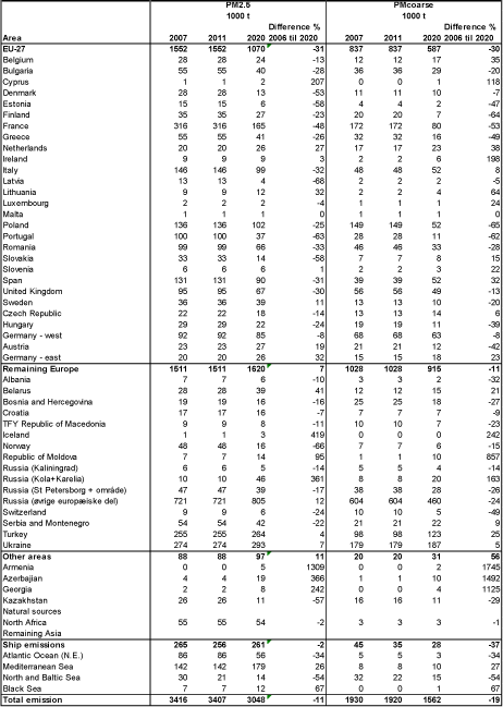
Table C.4: Emissions of NMVOC (non methane volatile organic compounds) from the land based sources used for the model calculations.
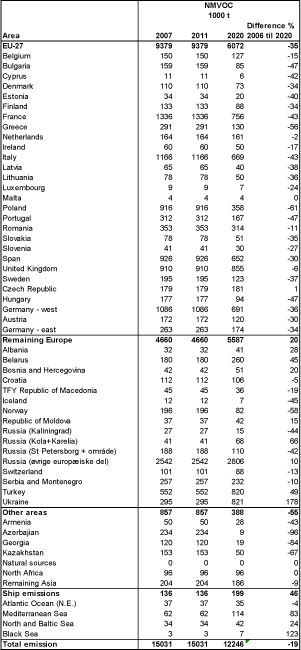
Version 1.0 October 2009, © Danish Environmental Protection Agency