Pesticides Research, No. 127, 2009
Buffer zones for biodiversity of plants and arthropods: is there a compromise on width?
Contents
- 2.1 Study site and experimental design
- 2.2 Weather
- 2.3 Yield
- 2.4 Vegetation recording
- 2.5 Arthropod recording
- 2.6 Data analysis
- 3.1 Flora
- 3.2 Arthropods
- 3.3 The marginal gain of diversity at increased buffer width
- 3.4 Combined flora and arthropod analysis
Appendix A: Field History and Treatments
Appendix B: Supplementary material on plants
Appendix C: Supplementary material on arthropods on woody plants in hedgerows
Appendix D: Supplementary material on arthropods observed by transect counts
Appendix E: Supplementary material on accumulated species richness in relation to buffer width
Appendix F: Statistical models
Appendix G: Local weather data
Preface
The present report “Buffer zones for biodiversity of plants and arthropods: is there a compromise on width?” on buffer zones along hedges represents a follow-up on a review publication from the Danish Ministry of Environment (Sigsgaard et al. 2007). That review addressed the potential use of various types of buffer zones to improve biodiversity and natural pest regulation in arable fields. The review publication established a need for research on the necessary dimensions of buffer zones, if such zones should become an operational and efficient tool to conserve biodiversity under pressure from intensive modern agriculture.
On this background, the Ministry of Environment made a call for research proposals among which the present project was financed. The project focuses on identifying a buffer zone width, which can both ensure a significant biodiversity increase and also be agriculturally feasible. The project has used plants, insects and spiders to measure biodiversity effects of different widths of buffer zones in spring barley.
The project has involved the following institutions and persons:
- Department of Agriculture and Ecology, University of Copenhagen (zoological expertise): Peter Esbjerg (Project leader), Lene Sigsgaard, Rasmus Nimgaard and Søren Navntoft.
- Department of Biology, University of Copenhagen (botanical expertise): Louise C. Andresen, Ib Johnsen, Niels Bruun, Jill Nothlev and Andreas Kelager.
- Department of Genetics and Biotechnology, University of Aarhus (statistical expertise): Kristian Kristensen.
The project group enjoyed current guiding discussions with an expert group:
- Jørn Kirkegaard (coordinator) and Lise Samsøe-Petersen, Environmental Protection Agency, Danish Ministry of Environment.
- Hans-Werner Griepentrog, Jannie Maj Olsen and Jacob Weiner, Dept. of Agriculture and Ecology, Univ. of Copenhagen.
- Lisa Munk, Dept. of Plant Biology and Biotechnology, Univ. of Copenhagen.
- Søren Marcus Pedersen and Jens Erik Ørum, Dept. of Food and Resource Economics, Univ. of Copenhagen.
- Lise Nistrup Jørgensen, Dept. of Integrated Pest Management, Univ. of Aarhus.
- Hanne Lindhard Pedersen, Dept. of Horticulture, Univ. of Aarhus.
- Poul Henning Petersen, Danish Agricultural Advisory Service.
- Niels Lindemark, Danish Crop Protection Association.
- Marc Trapman, BioFruitAdvices.
We thank the whole group for the collaboration.
The project was hosted by Gjorslev Estate. We owe the owner Peter Tesdorph sincere thanks for this possibility. The project layout and the treatments were managed in a most careful and competent way. For this we are very grateful to the Estate Manager Anders Bak Hansen and his most skilled Machine Operator Frank Holm. Without the skills and support from Peter Tesdorph and his staff this fairly complicated large scale project design could not have been carried out.
Summary
This report presents the results of a one-season field investigation of plant and arthropod biodiversity, as affected by the width of hedge-bordering buffer zones, maintained without application of fertilizers and pesticides. A review on buffer zones in arable fields (Sigsgaard et al. 2007) pointed at the effect of buffer width on biodiversity in and along agricultural fields as a question calling for attention. The Danish Ministry of Environment made a call for research projects; among other subjects on this aspect of buffer zones. The present project, which incorporated buffer zones of 4, 6, 12 and 24 m and a 0-m control was accepted, and started 2008. It included co-workers from University of Copenhagen (Department of Agriculture and Ecology and Department of Biology) and University of Aarhus (Department of Genetics and Biotechnology).
The aim of the project was to identify a buffer width which would significantly increase biodiversity in the field and in the hedge and which would also be agriculturally acceptable. For this, the effects of buffer zones of different widths were compared in order to investigate whether there is a compromise on width with respect to the increase in biodiversity and the agricultural feasibility. The buffer zones were placed along hedges in four large fields with spring sown barley at Gjorslev Estate on Eastern Zealand. In these zones, the hedge plant composition (woody species and dominant herbs) and their flowering was registered. This was followed by further plant species and plant density counts in the field. The plants’ flowering and generative stage were also noted. Insects and spiders were recorded by four methods three times during the season: beating tray sampling in hedges, transect counts of flying insects, sweep net sampling and pitfall trapping in the hedge-bottom and field areas.
Plants were identified mainly to species, and this was also the case for a considerable quantity of insects (e.g. butterflies, bumblebees, ground and leaf beetles, weevils and true bugs) while others were identified to genus, family or other well defined groups (e.g. small parasitic wasps). The plant and arthropod data were analysed in relation to buffer zone width and distance to the hedge. In addition, the effects of plant abundance and diversity were analysed for some arthropod taxa.
Both buffer zone width and distance to the hedge influenced plants and arthropods significantly. The abundance of wild plants in the field increased significantly and was more than doubled with a 6 m buffer zone compared to sprayed and fertilized field – an effect which to some degree continued with increased buffer width. Also the biodiversity of wild plants was increased with the establishment of buffer zones. 6 m of buffer was the minimum width required in order to significantly increase the plant biodiversity compared to plots without buffer area. There was a tendency towards increased biodiversity of wild plants at a further increased buffer width.
While the buffers only delivered limited protection of the hedge fauna, the buffer zone effects on the arthropod fauna within the hedge bottom (the vegetation beneath the hedge and out to the crop) and in the field were marked both in terms of increased abundance and in terms of increased biodiversity. For the arthropod abundance within the hedge bottom, a buffer width of 24 m delivered the most general increases, although in several cases a narrower buffer also resulted in higher abundances within the hedge bottom.
In the field (outside the hedge bottom) a significantly higher arthropod abundance was generally obtained with a 6 m or wider buffer zone. In addition, a generally and very markedly higher biomass of important bird chick-food items was found within the buffer zones at all distances from the field edge.
The biodiversity of arthropods within the hedge bottom increased consistently with a buffer zone width of minimum 6 m. This result was very clear and for the majority of the analysed taxa, a further increase in buffer width did not result in significantly higher biodiversity. This was further underpinned by the analysis of the marginal gain of biodiversity at increased buffer width, where it was found that the vast majority of the biodiversity increase within hedge and field was obtained already with a 6 m wide buffer zone.
Buffer zones had no effect on the flowering within the hedge bottom. The flowering percentages of wild plants in the field, however, was markedly higher within the buffer zones compared to treated field, and the importance of flowering was underlined by the significant positive correlations between flowering and activity of both butterflies and bumblebees.
An important spin off from this project is that butterflies seem to fulfil the role as a practical indicator for improvement of biodiversity. They responded positively to flowering, and positive correlations were found between biodiversity of butterflies and wild plants and between butterflies and other important arthropod taxa.
It is concluded, that irrespective of the slightly further increases of plant diversity and diversity of some arthropods at buffer zones widths of 12 m and 24 m, a 6 m buffer zone may be seen as a width providing a relatively high proportion of the biodiversity found at broader buffer zones in this one-year study. A 6 m wide buffer zone will also deliver a considerable amount of food resources for higher animals such as birds and small mammals.
For farmers, a 6 m buffer zone along hedges will primarily occupy a part of the field with some yield depression due to hedge competition. Furthermore, such a zone will increase the supply of food for game birds and hence open for an extra income.
For decision makers, the potential of a 6 m wide buffer zone along hedges, as a mean to counteract the negative effects of intensive modern farming on terrestrial biodiversity, should be both acceptable and somewhat attractive. 6 m buffer zones ought to open for subsidised regulation of biodiversity. In addition, monitoring of biodiversity effects should be possible using diversity of butterflies as indicator.
For an assessment of the full potential of buffer zones, future studies should include the performance of buffer zones present in field margins for more than one year. For such more permanent buffer zones, it will be important to include studies on vegetation management, and how vegetation management may further increase biodiversity of plants, insects and spiders, while avoiding that the buffer zones become a source of perennial weeds. It is also highly relevant to consider potential buffer zone effects on landscape connectivity by studying the effect of buffer area and the corridor effect for improved dispersal of flora and fauna by arranging coherent buffer zones over larger areas.
Sammenfatning
Rapporten beskriver resultaterne af en ét-årig undersøgelse af biodiversitetseffekten af forskellige bufferzone-bredder langs levende hegn i kornmarker. Bufferzoner er markstriber, som ikke er sprøjtet og gødet til gavn for vilde planter og dyr. En review-undersøgelse af bufferzoner i marker (Sigsgaard et al. 2007) afslørede et stærkt behov for at undersøge effekten af bufferbredde på biodiversiten i og nær landbrugsarealer. Dette spørgsmål var blandt de prioriterede i et udbud fra Miljøministeriet. Nærværende projekt blev accepteret og startede i 2008 med belysning af bufferbredder på 4, 6, 12 og 24 m. Projektet har involveret medarbejdere fra Københavns Universitet (Institut for Jordbrug og Økologi samt Biologisk Institut) og Aarhus Universitet (Institut for Genetik og Bioteknologi).
Projektet havde til formål at finde en bufferzone-bredde, som giver væsentlige forbedringer af biodiversiteten af vilde planter, insekter og edderkopper og som samtidig er landbrugsmæssigt acceptabel. De fire anvendte bufferbredder plus en 0-m kontrol blev placeret langs hegn i fire meget store vårbygmarker på Gjorslev Gods på Østsjælland. Hegnenes sammensætning af både vedplanter og urter samt urternes blomstring i fodposen blev opgjort, og i markarealerne blev opgjort plantearter, plantetætheder, blomstringsfrekvenser og generativ udvikling. Insekter og edderkopper blev opgjort via nedbankning fra hegn, ketcher-prøver, tælling af flyvende insekter i standardbaner og fangst i faldgruber.
Planter blev artsbestemt, og det samme gjaldt en stor del af insekterne (som f.eks. dagsommerfugle, humlebier, løbe-, blad- og snudebiller og tæger) mens andre kun blev identificeret til slægt, familie eller underorden (f. eks. små snyltehvepse). Planteforekomsternes sammenhæng med bufferbredde, afstand til hegn og flere andre faktorer blev analyseret statistisk. Forekomsterne af leddyr blev analyseret i forhold til det samme sæt faktorer samt i nogle tilfælde i forhold til planteforekomsterne.
Både bufferbredden og afstanden til hegn havde væsentlig indflydelse på planter og leddyr. Forekomsten af vilde planter i marken steg signifikant og blev mere end fordoblet med en 6 m bred bufferzone – en effekt der i nogen grad fortsatte med yderligere forøgelse af bufferbredden. Også biodiversiteten af vilde planter blev forøget med etablering af bufferzoner. En signifikant effekt på biodiversiteten krævede en bufferbredde på minimum 6 m sammenlignet med mark uden bufferzoner. En yderligere forøgelse af bufferbredden medførte en tendens til øget plantediversitet.
Mens effekten af bufferzonerne kun i behersket omfang kunne spores hos leddyrene på hegnenes vedagtige planter, var buffervirkningerne på leddyr i hegnenes fodpose (vegetationen under hegnet og ud til afgrøden) og i marken markante i form af øget antal og øget biodiversitet. For leddyrforekomsterne i hegnenes fodpose var en 24 m bufferzone den bredde, der gav den mest generelle antalsmæssige fremgang for de undersøgte grupper, men i flere tilfælde gav en smallere bufferbredde også antalsmæssig fremgang i hegnenes fodpose.
I marken (uden for hegnenes fodpose) var 6 m den smalleste bufferbredde, der gav en væsentlig og generel antals- eller aktivitetsmæssig fremgang på markfladen, men generelt steg mængden af leddyr med bufferbredden. Også biomassen af særlig egnet fugleføde steg generelt og særdeles markant i bufferzonerne i alle afstande fra hegn.
Biodiversiteten af leddyr i hegnenes fodpose blev markant forbedret med en 6 m bred bufferzone. Dette resultat var meget klart, og yderligere forøgelse af bufferbredden til 12 eller 24 m gav for flertallet af artsgrupperne ikke målbar biodiversitetsmæssig fremgang. At også den samlede biodiversitetsmæssige hovedgevinst af leddyr for hegn og mark set under et blev opnået allerede ved en 6 m bred bufferzone blev specielt tydeligt, når biodiversiteten målt i forhold til det samlede undersøgte areal (fra hegnet og ud i marken) blev analyseret.
Bufferzonerne havde ingen effekt på blomstringen i hegnenes fodpose. De vilde planters blomstring var derimod markant højere i bufferzonerne end i behandlet mark, og betydningen af denne blomstring blev understreget af de positive korrelationer mellem blomstringen og aktiviteten af både humlebier og sommerfugle.
Dagsommerfuglene synes at kunne fungere som indikator for biodiversitet. De responderede positivt på blomstring, og der var en positiv korrelation mellem biodiversiteten af dagsommerfugle og biodiversiteten af vilde plantearter, tæger og biller, som alle var vigtige målgrupper.
Det konkluderes, at uanset muligheden for et vist niveau af yderligere forbedringer af plante- og leddyrdiversitet ved bufferbredder på 12 og 24 m, er forbedringerne, der opnås ved en 6 m bufferbredde, biodiversitetsmæssigt attraktive, og 6 m kan ses som en bredde, der giver en relativ høj mætning mht. biodiversitet. En 6 m bred bufferzone vil også bidrage med et betydeligt ekstra fødegrundlag for højerestående dyr som fugle og mindre pattedyr.
For landbrugere burde 6 m subsidierede bufferzoner langs hegn udgøre et acceptabelt og i nogen grad attraktivt tiltag. Således vil en 6 m bred bufferzone langs hegn falde på et areal, hvoraf en væsentlig del er udbyttebegrænset af konkurrencen fra hegnet. Hertil kommer, at bufferzonens positive effekt på mængden af føde til kyllinger af agerhøne og fasan vil medføre muligheder for øgede jagtindtægter.
For de politiske beslutningstager kunne anlæg af bufferzoner udgøre en interessant mulighed for at opnå en subsidieret modregulering af landbrugets negative biodiversitetseffekter. Tilmed kan biodiversitetsgevinsten ret overkommeligt effektmoniteres ud fra forekomsten af dagsommerfugle.
Hvis bufferzoners fulde potentiale skal udnyttes, vil det være vigtigt at finde frem til det areal af 6 m bufferzoner, der kræves for at opnå en markant positiv effekt på biodiversiteten på landskabsniveau. Også effekten af tid, og hvordan den videre håndtering/ pleje af vegetationen i bufferzoner bedst fremmer biodiversiteten og beskytter landbruget mod uønsket ukrudt, bør undersøges. Bufferzoner vil typisk ligge i mere end et enkelt år, og biodiversiteten må herved forventes yderligere øget.
Det vil også være vigtigt at overveje og belyse, hvilke korridor-muligheder der vil være for at opnå en forbedret og ønskelig spredning af arter, hvis sammenhægende bufferzoner placeres hensigtsmæssigt over lidt større landskaber.
1 Introduction
1.1 Background
In the discussion of the fate of biodiversity in the modern landscape the role of intensified agricultural production and particularly the use of chemical inputs attract much attention. Through analysis of data over 30 years in the UK, Benton et al. (2002) found that the decline in bird populations are correlated with declining insect populations, caused by agricultural intensification. Also in Denmark the improvements of crop yield and quality are at the expense of biodiversity in the arable fields (Andreasen et al. 1996; Kudsk & Streibig 2003; eds. Esbjerg & Petersen 2002, Navntoft et al. 2003), and the use of insecticides has in 1998 (Grell 1998) been suggested as a major factor behind the decline of Danish breeding birds. The British Game Conservancy Trust financed experiments with unsprayed field margins in order to increase the numbers of birds of game. Important effects were demonstrated on bird food insects for the field living birdlife such as Grey Partridge and Pheasant but also butterflies benefitted from non-treated 6 m field margins (Potts 1986, Sotherton 1987, Sotherton et al. 1989). A parallel Danish investigation of effects on flora and insects of 6 m non-sprayed field margins along hedgerows found improvements for both plants and insects (Hald et al., 1988). Later Esbjerg & Petersen, eds. (2002) demonstrated increases of wild flora species, flowering plants, insect and bird abundances at half and particularly quarter dosages of herbicides and insecticides. With conversion to organic farming a further increase in flowering plants and higher presence of butterflies was found, and the concomitant increase of weed seeds and arthropods was followed by a doubling of Skylarks in the organic fields (Navntoft et al. 2003).
The above findings, and the suggestions of Marshall (1989) and Wilson & Aebisher (1995), that hedgerows are important for the wild flora abundance, make hedges and field margins along them an interesting study area for biodiversity improvements. Many studies have looked into different aspects of field margins and others have looked into the potential use of flower strips and beetle banks, mostly with improvement of pest regulation by predators and parasitoids as the focus area.
Despite many demonstrations of predation (e.g. Collins et al. 2002, Collins et al. 2003) the demonstration of direct benefits to farmers at field level have failed except in a very few cases (e.g. Östman et al. 2003).
In contrast to this, the indications of biodiversity improvements are many but the approaches are mostly agriculturally focussed and very mixed in terms of both methodologies and terminologies. This was underlined by a review of buffer zone approaches mainly in Europe (Sigsgaard et al. 2007). Most remarkable was the fact that most buffer zone dimensions seemed to be selected somewhat arbitrarily.
At the administrative level, non-treated field margins is one of the targets of agricultural subsidies in several EU-countries. However, the width of the margin requested varies between countries (Sigsgaard et al. 2007). In this light, and on background of the general concern about biodiversity in farm landscapes, it is interesting that nobody has yet asked if it is possible to find a margin width, which will on one hand ensure a high saving/ improvement of biodiversity, and on the other hand will be tolerable for practical agriculture. Sigsgaard et al. (2007) among others point at the need to further investigate the influence of width and area of buffer zones.
In the current study, we investigated the biodiversity effect of non-fertilized and pesticide free buffer zones bordering hedgerows in order to fulfil the below aims.
1.2 Aims and hypotheses
The project takes some initial methodological steps towards a more systematic analysis of the importance of pesticide and fertilizer free buffer zones along hedgerows, here defined as field margins with one or more rows of woody plants, for improved biodiversity in agricultural landscapes. The project focuses on the impact of a simple set of different buffer widths (4, 6, 12 and 24 m).
AIM AND HYPOTHESES
The aim of the investigation was to identify a buffer zone width which would deliver a significant improvement of biodiversity (measured as species richness and a biodiversity index) from which an additional increase in width would only lead to marginally higher biodiversity. This aim was based on the two hypotheses below, which should be regarded as interconnected:
- The biodiversity of plants and arthropods in a buffer zone along a hedgerow will increase with increasing width of the buffer zone, until a substantial saturation level is reached. Further increase of the width will only yield a relatively limited further increase of biodiversity.
- It will be possible to identify an agriculturally practicable buffer zone width along hedgerows which will benefit flora and fauna so much, that the abundance and biodiversity will increase significantly.
Furthermore, an important part of this project was to identify organisms which may serve as suitable bioindicators for biodiversity improvements caused by buffer zones in arable fields.
2 Methods
- 2.1 Study site and experimental design
- 2.2 Weather
- 2.3 Yield
- 2.4 Vegetation recording
- 2.5 Arthropod recording
- 2.6 Data analysis
In order to investigate the influence of buffer zone widths on biodiversity, we have tried to reduce the often challenging variation caused by using different farms over several years. Therefore, the whole experiment took place within one season at one large estate, Gjorslev Gods, on eastern Zealand. Gjorslev provided study facilities in four large spring barley fields with basically the same type of hedge composition with a herbaceous hedge bottom along the eastern side of the fields. The hedgerows had the same geographical orientation (north-south hedges). The size of the fields permitted the establishment of the necessary plot sizes within each field. The fertilization and spraying within the experimental plots was handled solely by the Farm Manager and one very experienced machine operator.
The biological work consisted of the following main parts:
- Characterisation of the hedgerows (dimensions, composition of woody species and their flowering frequency)
- Recording of all plant species in the fields and along the hedges, and in addition assessment of plant densities and flowering density.
- Transect counting of selected insects such as butterflies and bumblebees.
- Pitfall trapping of epigaeic beetles and spiders with focus on beneficials (natural enemies of pests).
- Sweep net sampling of insects on plants designed to permit estimates of abundance, biodiversity and bird prey.
- Beating tray samples of insects from hedges designed for obtaining abundance and biodiversity estimates.
Table 2. 1. Schematic summery of sampling times of wild flora and arthropods in hedge, hedge-bottom and field. Vegetation recording: 1) hedge dimensions, 2) hedge woody species composition, 3) hedge woody species flowering intensity, 4) coverage of hedge-bottom herbs 5) coverage of flowering and generative hedge-bottom herbs, field assessment of 6) number of Herbs and 7) number of flowering and generative Herbs. Arthropod recordings: 8) Pitfall trapping of epigaeic arthropods, 9) sweep net sampling of herbaceous dwelling arthropods, 10) transect counts of butterflies and bees and 11) arthropods sampled from woody hedge components.
| Biotope | May, Period 1 | June, Period 2 | July, Period 3 |
| Hedgerow | 1, 2, 3, 11 | 3, 11 | 3, 11 |
| Hedge-bottom | 4, 8, 9 | 4, 5, 8, 9 | 4, 5, 8, 9 |
| Field | 6, 8, 9, 10 | 6, 7, 8, 9, 10 | 6, 7, 8, 9, 10 |
In Table 2.1 the sampling schedule of all data samplings is presented. Further details on the different methodologies are given in the subsequent sections of this chapter.
2.1 Study site and experimental design
The study was carried out as a single year field study at Gjorslev Estate in 2008.
2.1.1 Gjorslev Estate
Gjorslev Estate (Gjorslev vej 20, Holtug, 4660 Store Heddinge, Denmark, coordinates (wgs84): 55°21’14.34”N, 12°22’51.93”E) covers 1.668 ha of which 753 ha is forest. Gjorslev was asked to host the trial because of its large field sizes with well established homogeneous hedgerows. Large fields with long uniform hedgerows were needed in order to establish the required experimental design (section 2.1.2). An aerial view of a part of Gjorslev is presented in Fig. 2.1.
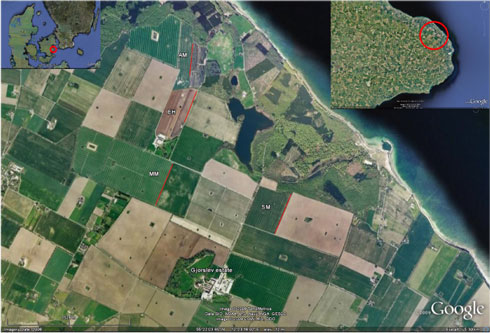
Fig. 2.1. Areal view of the four experimental fields At Gjorslev Estate: Møllemark (MM), Enghaven (EH), Anders mark (AM) and Skovmark (SM). The positions of the experimental parts of the hedgerows are indicated with red lines. The area is characterised by Large Fields in a relatively Heterogenous landscape with forest, lakes, running water and sea shore. As an indication of scale, the experimental area in Møllemark (MM) is 543 m long.
2.1.2 Experimental design
Four fields were included in the experiment (Fig. 2.1). In Fig. 2.2 an outline of an experimental field is presented. Data were collected on the western side of the eastern hedgerows in all fields. Along each hedge there were five treatments consisting of areas treated with neither fertilizer nor pesticides in 2008 – called buffer zones. The widths of the zones were 0, 4, 6, 12 or 24 m and they were arranged in chronological order for easier and more reliable management (Fig. 2.2).
Fig. 2.2. Outline of an experimental block within an experimental field. The trial included four such areas. There were five experimental plots within each block, each being 80 – 108.5 m long depending on the length of the hedgerow used in each field. The plot arrangement within a field was not randomized but was arranged at descending width of the buffer zone. However, within each field it was randomized whether the widest buffer zone of a field should be placed north or south. Five rows of sampling points perpendicular to the field edge were established for each experiment and were between 12.5 and 19.6 m apart depending on the plot length. The first and last sampling row within each plot was placed 15 m from the plot edge to lower interference from neighbour plots or ordinary field. Plant and arthropod sampling along each sampling row was carried out in the hedge bottom (ref. distance 0) and then 2, 5, 9 and 18 m within the field from the field edge (red squares). This sampling grid contained in total 25 sampling points per plot (5 × 25 = 125 pr. field). Additionally plant and arthropod recordings were carried out within the hedgerow.
The various buffer zones (treatments) are referred to as buffer 0 (0 m buffer), buffer 4 (4 m buffer) etc. It is important to emphasize that when the term “buffer 0 – 24” is used, it is the entire experimental plot area (in some cases at a specific distance from hedge) that is referred to and not only the width of the buffer strips (see Fig. 2.2). Hence, the size of the sampled area was always the same and it is only the ratio between treated and non-treated areas that varies.
The experiments were always surrounded by a section of ordinary field or headland. In both SM and MM the almost full length of the fields were included in the experiment and only guarded by 24 m of headland in both ends, as the field and the neighbour area on the western side of the hedgerow was fairly homogenous. In EH only the Northern end of the field was used, as the southern end was relatively low and often flooded during spring. This field was therefore guarded by 24 m of headland towards North and by approximate 200 m of field in the southern part. The experimental block in AM was placed along the middle of the hedgerow, thereby avoiding bordering up to a forest in the Northern part and a low waterlogged area in the Southern end. The experimental area AM was therefore bordered by 214 m toward North and 157 m toward South.
In SM and MM parts of the hedgerows had no trees or shrubs but herbs or grasses only. In SM this part was located in buffer 12 and comprised 30 m bordering to buffer 6. In MM buffer 24, 14 m were without woody plants. For more information on the hedgerows see section 3.1.1.
After randomization, the widest (24 m) buffer zone was placed at the northern end of the hedge in SM, MM and AM and at the southern end in EH. The plots in SM were 104.5 m long, 108.5 m in MM and 80 m in both EH and AM.
2.1.3 Pesticide and fertilizer applications
The four fields were treated identically with respect to the cultivation procedures, including fertilizing, sowing and pesticide application. The crop (spring barley cv. Henley) was sown relatively late in April due to wet soils. Right before sowing, liquid ammonia fertilizer was placed very accurate (injected) within the treated areas of the experimental plots. Later ammonium sulphate was applied (by rotary spreader) to the treated areas (for more information on fertilizer applications see Appendix A). Three weeks after sowing, a mixture of herbicides and fungicides was applied using low-drift (yellow) nozzles along with manganese sulphate. Eight weeks after sowing a mixture of fungicides and insecticides was applied (see Appendix A). Three weeks later, another insecticide treatment was carried out. The crop was harvested mid August (For more information on the pesticides and other field treatments see Appendix A). The pesticide dosages were normal according to the Danish Agricultural Advisory Service and close to the mean of 2008 (Miljøstyrelsen 2009).
2.2 Weather
The weather in spring (March, April and May) 2008 can be summarised as sunny and warm (dmi.dk/dmi/vejret_i_danmark_-_foraar_2008). The mean temperature in Denmark was 7.9ºC which is 1.7ºC above the average of the period 1961-90 but 1.1ºC lower than the same period in 2007. The mean precipitation in Denmark in spring 2008 was 131 mm which was 3 mm below the average of 1961-90. Denmark had 663 h of sunshine in spring 2008, which is the sunniest spring since the recording started in 1920.
The summer (June, July and August) in 2008 was sunny, wet and mild (dmi.dk/dmi/vejret_i_danmark_-_sommer_2008). The mean temperature in DK was 16.4ºC which is 1.2ºC above the average of 1961-90. The last half of July was very warm with several days above 25ºC. The mean precipitation was 240 mm which was 52 mm or 28% above the mean of 1961-90, although by far the highest amount of rain fell in August. Denmark had 721 h of sunshine in summer 2008, which is 130 h or 22% above the mean of 1961-90.
We measured the weather at Gjorslev using a local weather station (Hardi Klimaspyd) placed in the centre of the experimental field SM (Skovmark). These local weather data can be found in Appendix G.
2.3 Yield
The average barley yield in the experimental fields in 2008 was 72 hkg ha-¹ (79 hkg in SM, 72 hkg in MM, 76 hkg in EH and 59 hkg in AM). Yield losses within the buffer strips was not measured, however, according to the farm manager the yield in the buffer zones was assessed to be less than half the yield in the ordinary field (A.B. Hansen pers. comm.).
2.4 Vegetation recording
2.4.1 Hedgerow
Plant species composition of the hedgerows was assessed for all woody species and dominant herbs with 1 m resolution. The woody species were assessed once at May 7th and the dominant herbs were assessed at three runs commencing May 7th, June 19th and July 17th. The dimensions of the hedge were measured once at May 7th with total height, height of bank and total width. Flowering intensity was determined for the dominant flowering woody species: May 7th to 12th for hawthorn (Crataegus spp.) and June 19th for rose (Rosa spp.). Inflorescences (Crataegus) and number of flowers (Crataegus and Rosa) were counted on three 50 cm long branches in each plot. The value of the plants as pollen and nectar sources was recorded according to The Danish Beekeepers´ Association (Svendsen 1994).
2.4.2 Hedge bottom and field
In two sampling runs, 27 May - 12 June and 6 – 16 July respectively, vegetation was registered after the experimental fields had been sprayed with herbicides. At the distances 0, 2, 5, 9 and 18 m from the field edge (Fig. 2.2), 10 vegetation frames (Fig. 2.3) were used for density counts and for plant species (when possible) or genus recording according to Frederiksen et al. (2006). The frames were 40 × 50 cm², and divided into 20 sub-quadrants. Within the hedge bottom, density counts were not possible, and instead percent ground cover of each species/genus was recorded. At the second sampling run, flowering and generative stages of the plants were registered. The frames were always placed adjacent to one pit-fall (Fig. 2.3). Furthermore, 40 m from the hedge, 12 vegetation frames were sampled for additional information.
At the first sampling run, the number of spring barley plants was counted in all vegetation frames in four of the 20 sub-frames. The growth stage of spring barley was assessed according to the BBCH scale (Tottman & Broad 1987). Furthermore, the height and percentage cover of spring barley was registered, in treated and non-treated areas.
2.5 Arthropod recording
Arthropod sampling was carried out in each of three sampling periods in 2008: Period 1 was after herbicide and fungicide application (May – early June). Period 2 was after the first insecticide and fungicide application (June – early July). Period 3 was after the second insecticide application (July).
2.5.1 Hedgerow
Arthropods were sampled on the woody plants of the hedgerows using a beating tray sampling technique. The sampling was carried out in May (28 May 2008), June (18 and 20 June 2008) and July (14 and 15 July 2008). Samples were collected in the five buffer zones per field along the west side of the hedges of the four experimental fields.
A beating sample was the sum of beating 1branch of 10 individual trees of the same species. Each branch received three firm beats. Arthropods were collected in plastic bags attached to the opening of the tray funnel. Samples were labelled with date, locality, buffer zone width, woody plant species and sample number.
The total number of samples per treatment was between 9 and 11 in order to accommodate that at least two samples were collected from each of the selected woody species present within a treatment (the average number of trees per combination of sampling time, field and buffer width was 9.6). In Andersmark, which was dominated by rose, it was not possible to obtain two samples pr treatment from the only other available species, hawthorn. The total number of samples was 576.
The faunal composition and total number of arthropods depends on the woody plant species. To obtain a correct picture of changes over time, and to be able to compare data from different treatments and fields, arthropods were only collected from the most common woody species available for sampling (it must be possible to reach and beat branches) in the four fields. In three of the fields, the woody species sampled were blackthorn (Prunus spinosa), elderberry (Sambucus nigra) hazel (Corylus avellana) and hawthorn (Crataegus spp.). However, the hedgerow of the fourth field, Andersmark, was strongly dominated by roses (Rosa spp.), with a few hawthorn interspersed, and only these two species were sampled in this hedgerow. Though present, it was not possible to sample from roses in the other three fields, as the roses in these fields were growing inside the hedgerow, and were not accessible for sampling.
Samples were kept in cooling boxes in the field. Cooling boxes maintained samples near 12oC, hereby reducing deterioration as well as arthropod activity, hence the risk of predation in the samples. In the laboratory samples were kept at -20oC until sorting and identification to order, family, genus or species under the stereomicroscope (see Table C.1 in Appendix C). All arthropods were named according to Fauna Europaea 2009 (http://www.faunaeur.org/index.php).
For important bird food items, the fresh weight was determined as a quantitative measure of the amount of bird food. For details on arthropod prey included as bird food see section 2.5.2.2.
For each sample, the woody species was recorded and the number of arthropod species was counted. The number of species was summed over the samples in each plot and Shannon’s indexes were averaged over the trees in each plot. Shannon’s biodiversity index was calculated for each combination of sampling time, field and buffer width (see section 2.6).
2.5.2 Hedge bottom and field
Three different sampling methods were used in order to cover arthropod populations of flying (avian), herbaceous dwelling and ground dwelling (epigaeic) species.
2.5.2.1 Transect counts of butterflies and bees
Standardized transect counts of Lepidoptera (butterflies) and Apidae (bees) were carried out following a method by Pollard (1977) and Pollard & Yates (1993) in order to estimate the activity of these insects in relation to buffer zone width.
Insect counts during systematic walks along the fields (transects) were carried out 2, 5, 9 and 18 m from the field edge. The 2 m distance census area was 4 m wide. It covered the hedgerow and 4 m into the field. In the relatively narrow 4–6 m strip (see Fig. 2.2) the census area was only 2 m wide. At the 9 and 18 m distances the census area was 4 m wide. In all cases the census area in front of the observer was 5 m long. The order of field visits, the starting points of the transect walks (North or South) and the order of the starting distance from the field edges were all randomised. Care was taken not to count an individual more than once, however, in doubtful cases or if an individual came from behind of the observer, it was always counted as a new individual. If the identity of an individual was uncertain, it was caught with a butterfly net and identified to species.
The observer spent 5 – 15 minutes walking through each census area of a plot. The time spent for each plot within a field was kept approximately uniform and was always registered.
Transect counts were preformed during three periods with three or four replicates in each of the four fields. Period 1: 27 May to 4 June. Period 2: 25 June to 11 July. Period 3: 24 – 31 of July. In total 40 transect counts were carried out. The earliest transect count began at 10.37 and the latest transect count ended at 18.14 (Greenwich Mean Time + 2 h). Wind speed (m/s at 24 m from the hedgerow), sunshine (on a scale from 0 – 4 with 0 representing full sun and 4 completely clouded) and temperature (ºC) were all registered. The wind speed never exceeded 6.5 m/s and the temperature was always above 17 °C during transect counts. If rain set in, the counting was abandoned and a new attempt was made the next day. During each period, one set of transect walks were completed in each of the four fields before starting the next sampling round. Each round lasted no more than three days.
2.5.2.2 Sweep net sampling of arthropods in the herbaceous vegetation
Herbaceous-dwelling arthropods like butterfly larvae and leaf beetles were sampled using standard sweep nets (diam. 27 cm). One sample (10 standard sweeps) was taken at each of the 25 sampling points per plot (see Fig. 2.2) on three occasions. The first sampling occasion was 2-3 June, 12-13 days after herbicide and fungicide applications. The second sampling round was carried out 24-26 June, 7-9 days after the first insecticide and fungicide application. The third and last sampling occasion was 15-16 July, 13-14 days after the second insecticide application. In total 1500 sweep net samples were collected.
The catch from each sample was put in a plastic bag, labelled and placed in a cooling box until it was frozen at -20ºC later the same day. In the laboratory all arthropods were counted and identified at least to order. The majority of, taxonomic units were identified to species (see Table D.20 in Appendix D). All arthropods were named according to Fauna Europaea 2009 (http://www.faunaeur.org/index.php).
Chick-food items
In order to identify buffer zone effects on the availability of arthropod food for higher trophic levels, arthropods being important as chick-food (see Wratten & Powell 1991, Sotherton & Moreby 1992, Petersen & Navntoft 2003) from the sweep net samples were grouped and weighed per sample (g fresh biomass after de-frosting): Araneae, Opiliones, Coleoptera (except Coccinellidae and Cantharidae), Hemiptera, Lepidoptera (larvae only), Tenthredinidae (larvae only), Syrphidae (larvae and pupae only), Orthoptera and Neuroptera.
2.5.2.3 Pitfall trapping of epigaeic arthropods
Carabidae (ground beetles), Staphylinidae (rove beetles), Araneae (spiders) and other epigaeic arthropods were sampled with pitfall traps (plastic cups, diameter 82 mm, depth 70 mm, with snap-on lids) buried flush with the soil surface. The traps were partly filled with 200 ml of trapping and preservation fluid (a mixture of 1:1 ethylene glycol and tap water, with one drop of non-perfumed detergent per 10 l). In total 25 traps were used per plot (see Figs. 2.2 and 2.3). Three sampling rounds were carried out. The first set of traps were started 28 May (six days after herbicide application, see Appendix A for pesticide details). The second set of traps was started 18 June (one day after the first insecticide application) and the third set of traps was started 11 July (nine days after the second insecticide application). The first sampling round lasted 48 h and the second and third 72 h before the traps were collected, labelled and stored at 5°C until further processing. In total 1500 pitfall samples were collected. In the laboratory arthropods belonging to Araneae (spiders), Carabidae (ground beetles), Staphylinidae (rove beetles) and a few other taxa were counted and identified at minimum to family but preferably to species (see Table D.24 in Appendix D)
2.6 Data analysis
In addition to the actual recorded number of individuals, two measures were calculated in order to access the biodiversity: The number species (species diversity) and Shannon´s biodiversity index, H (Magurran 2004). Shannon´s H was calculated as:
Both measures were calculated and analysed for selected groups of plants and arthropods.
In order to estimate and test the effects of buffer width, distances from hedge and in some cases sampling time, the data were analysed statistically. The applied statistical methods and models depended to a large extent on the type of data, so that linear mixed models were used for data that could be assumed to be normally distributed such as weights, Shannon´s biodiversity index and log-transformed number of species, while counts and relative counts that could be assumed to be Poisson distributed and binomial distributed, respectively, were analysed using generalised linear mixed models. The random effects included in the models reflect that each field could be regarded as a complete block (replicate) in the same experiment – an experiment that is regarded as a split-block design. The actual applied models are explained, shown in a mathematical form and listed in Appendix F. In the following, the models are described very briefly with reference to the detailed description in Appendix F. The theory of linear mixed models and generalised linear mixed models may be found in books such as McCulloch and Searle (2001) and West et al. (2007). All statistical analyses were performed using the procedures MIXED, GLIMMIX and NLMIXED of SAS (SAS, 2008). Some of the results were visualised using the graphical procedures of SAS (SAS 2009a and SAS 2009b).
2.6.1 Flora analyses
The number of counted plants at each sampling period was analysed using generalised linear mixed models. The analyses were carried out for the different sampling period and groups (all, type and family) of plant species. The fixed effects in the model depended on the source of the data: field or hedge. For data from the hedge the model included the fixed effect of field and buffer width (Model 6 of Appendix F). For data from the field the model included the fixed effect of field and buffer width, distance to hedge and the interaction between buffer width and distance (Model 8 of Appendix F). The data from the field were also analysed in models, where the effect of buffer width and distance to hedge were treated as continuous variable using a second degree model (Model 12 of Appendix F). This model was then subsequently reduced by removing non-significant effects in order to get a model as simple as possible. The percentage of flowering plants at the second sampling run were analysed using a generalised linear mixed model including the effect of field and buffer width, distance to hedge and the interaction between buffer width and distance (Model 9 of Appendix F). The percent flowering plants in hedge-bottom at the second sampling run was calculated from the sum over coverage of all plants and flowering plants for each combination of field and buffer width. The log-transformed values were analysed in a linear model including the effect of field and buffer width as fixed effects (Model 13 of Appendix F).
Shannon´s index and the number of species (after log-transformation) were analysed in different models. Initially the data were analysed in a linear mixed model. The effect of location (control recordings in “the middle” of the field versus plots close to the hedge) together with the following three effects: ¹) distance to hedge, ²) width of buffer zone and ³) the interaction between distance to hedge and width of buffer zone. The model also included the effect of sampling period and interactions with sampling period (Model 14 of Appendix F).
In order to evaluate the distance at which Shannon's index was reduced to half its value at the hedge, the difference between its value in the hedge and its value in “the middle” of the field was also modelled using the logistic function. Two versions of the models were used: ¹) where it was assumed that decrease per unit (log distance) were the same for all buffer zones and ²) where it was assumed that decrease per unit (log distance) depended on the buffer zone (Model 5 of Appendix F).
2.6.2 Arthropod analyses
2.6.2.1 Hedgerow
The different groups of arthropods in the beating tray samples at each sampling period were analysed in a generalised linear mixed model including the fixed effect of field, buffer width and tree species (Model 7 of Appendix F) whereas the weights of bird feed at each sampling time were analysed using a linear mixed model including field, buffer width and tree species as fixed effects (Model 4 of Appendix F).
2.6.2.2 Hedge bottom and field
Transect counts of butterflies and bees
The number of individuals for different groups of arthropods were analysed separately for each sampling period using a generalised linear mixed model that included the fixed effect of field and buffer width distance to hedge and the interaction between buffer width and distance. In order to adjust for time spent in the transect, day and time of sampling and the other conditions for activity (e.g. temperature) the logarithm of the time spent in the transect was includes as an offset variable, the actual day was included as a fixed effect while the linear and quadratic effects of the following variables were included as covariates (fixed continuous effects): time of day (hours before or after noon), amount of sun (on a scale from 0 to 4 with 0 being full sun (no clouds) and 4 being fully overcast) and temperature (°C). This model was then reduced step by step by removing non significant covariates. The full model is Model 10 of Appendix F.
Shannon´s index (see section 2.6) and number of species (after log-transformation) for selected groups of arthropods were analysed using a linear mixed model including the fixed effects of buffer width, distance to hedge, sampling period and all 2- and 3-way interactions between these (Model 2 of Appendix F).
Sweep net sampling of herbaceous dwelling arthropods
The data were aggregated over replicates before analyses in order to decrease the number observations with zero target arthropods. Different groups of arthropods at different sampling periods were analysed using a generalised linear mixed model that included the fixed effect of field, buffer width, distance to hedge and the interaction between buffer width and distance (Model 8a in Appendix F).
The weight of bird feed at each sampling period were analysed in a linear mixed model including the fixed effects of field, buffer width, distance to hedge and the interaction between buffer width and distance (Model 3 of Appendix F).
Shannon´s index and number of species (after log-transformation) for selected groups of arthropods were analysed using a linear mixed model including the fixed effects of field, buffer width, distance to hedge, sampling period and all 2- and 3-way interactions between buffer width, distance to hedge and sampling period (Model 2 of Appendix F)
Pitfall trapping of epigaeic arthropods
The data were aggregated over replicates before analyses in order to decrease the number observations with zero target arthropods. Different groups of arthropods sampled were analysed separately at each sampling time using a generalised linear mixed model that included the fixed effect of field, buffer width, distance to hedge and the interaction between buffer width and distance (Model 8a of Appendix F).
Shannon´s index and number of species (after log-transformation) for selected groups of plants were analysed using a linear mixed model including the fixed effects of field, buffer width, distance to hedge, sampling period and all 2- and 3-way interactions between buffer width, distance to hedge and sampling period (Model 2 of Appendix F)
2.6.3 Combined flora and arthropod analyses
2.6.3.1 Activity of Lepidoptera (butterflies) and Bombus in relation to flower and host plant abundance
In order to evaluate the effect of plants on the occurrence of selected groups of arthropods, avian species from transect data were analysed in a second model. This second model included the same fixed effects as the model for transect data (Model 10 of Appendix F) together with linear and quadratic effects of the following variables: number of host plants (or coverage of host plants)and number of flowers for selected or all plant species (Model 11 of Appendix F). The full model was reduced step by step by removing non significant variables.
2.6.3.2 Analyses on the marginal gain of biodiversity when increasing buffer width
For wild plants and selected arthropods groups (Heteroptera, herbivorous coleopterans, Carabidae and Lepidoptera), the total number of species in each of the distances ranges 0, 0-2 m, 0-5 m, 0-9 m and 0-18 m was summarised for each combination of field and buffer width. Woody species in the hedge rows were not included in the plant analyses. Lepidoptera (butterflies) were not analysed for distance 0 m, as this distance was included in distance 2 m during data recording.
The number of species from each of those distance ranges were analysed in a linear mixed model (after log-transformation) including the effect of field and buffer width (Model 13 of Appendix F). These analyses were carried out on the July data comprising hedge bottom and field area (sampling run 2 for plants and sampling period 3 for arthropods) where the experimental plot had received the full fertilizer and pesticide effects.
The data for all buffer widths were also analysed in a non-linear model (Model 15 of Appendix F) to estimate the species – area relationship (SPAR). Arthropod data from the woody species in the hedgerows were included in the modelling, however, the distances in the hedgerow (hedge bottom versus hedge row) were analysed as one distance (dist. 0) in this model to make them fit into the assumed species – area relationship. The area for each distance was counted as the unit 1. Data were summarized across all sampling times in order to reveal buffer effects on biodiversity comprising the entire season.
2.6.3.3 Lepidoptera (butterflies) as bioindicator for biodiversity gains of buffer zones
The data for selected group of arthropods were analysed in a generalised linear model in order to examine the possible correlation between arthropod species diversity and species diversity between arthropods and dicotyledons. In order to avoid that the possible correlation was introduced by the difference between treated and untreated plots, the model include the effect of treatment as fixed factor as well as possible significant effect of field. The model also allowed the correlation to depend on whether the plots were treated or untreated (for more details see Model 16 in Appendix F).
3 Results
- 3.1 Flora
- 3.2 Arthropods
- 3.3 The marginal gain of diversity at increased buffer width
- 3.4 Combined flora and arthropod analysis
3.1 Flora
3.1.1 Hedge
The hedgerows (Appendix B, Table B.3.) of the four fields, did not differ significantly with respect to species composition for woody plants (P=0.9457, one-way ANOVA) or for dominant herbs (P=0.7365; P=0.9010 and P=0.7532 respectively for each sampling run). However, despite the lack of statistical difference, the hedge in AM differed from the other three hedgerows by being dominated by roses (Rosa spp.) (see Table B.3 in appendix B).
3.1.2 Hedge bottom and field
All plant species present in the field and the hedge-bottom are presented in Appendix B, Tables B.1 and B.2 with the abundance given for each combination of distance and buffer zone width. Results of the statistical analysis on weed densities in the field are presented in Table 3.1. The densities of all recorded weeds in the field are presented in Fig. 3.1. The figure shows no change in number of weed plants with distance from the hedge, with a buffer width 0 m. At buffer 24, however, the number of weed plants increased with proximity to the hedge. Increasing buffer width resulted in higher number of weeds with distance from the hedgerow.
Table 3.1. Schematic summary of the statistical analyses on abundance of the wild flora in the field at the second sampling run in July. Monocots are all individuals of the monocotyledonous species , Dicots are all individuals of dicotyledonous species.
| Order | Family | Run² | Test results F(ndf,ddf)P¹ | |||
| Field³ | Distance4 | Buffer5 | Buffer × Distance6 |
|||
| Monocots | All | 2 | 21.31(3,14)*** | 5.52(4,11)* | 5.05(4,12)* | 1.99(16,52)* |
| Poaceae | 2 | 21.31(3,14)*** | 5.52(4,11)* | 5.05(4,12)* | 1.99(16,52)* | |
| Dicots | All | 2 | 13.36(3,12)*** | 6.77(4,11)** | 8.08(4,16)*** | 5.16(16,43)*** |
| Apiaceae | 2 | 51.15(3,16)*** | 4.49(4,7)* | 0.76(4,8) NS | 6.85(16,52)*** | |
| Asteraceae | 2 | 4.57(3,11)* | 15.54(4,15)*** | 3.08(4,55)* | 2.63(16,47)** | |
| Brassicaceae | 2 | 2.83(3.20)NS | 2.45(4,13)NS | 3.49(4,16)* | 3.90(16,51)*** | |
| Chenopodiaceae | 2 | 20.66(3,9)*** | 3.26(4,7)NS | 7.20(4,11)** | 4.99(16,55)*** | |
| Lamiaceae | 2 | 3.83(3,16)* | 7.93(4,13)** | 2.88(4,26)* | 1.55(16,51) NS | |
| Scrophulariaceae | 2 | 0.67(3,14)NS | 3.07(4,11)NS | 0.86(4,19) NS | 3.63(16,47)*** | |
| Violaceae | 2 | 9.94(3,16)*** | 0.91(4,11) NS | 2.06(4,11) NS | 3.33(16,45)*** | |
| All | All | 2 | 30.14(3,13)*** | 9.86(4,14)*** | 14.48(4,62)*** | 3.61(16,62)*** |
¹ NS not significant, *P < 0.05, **P < 0.01, ***P < 0.001, F is the F-value, ndf and ddf is the numerator and denominator degree of freedom used for testing the significance.
² The second sampling round was carried out from 24 June.
³ Effect of field (four fields were included in the experiment).
4 Effect of distance from field edge (sampling was carried out 2, 5, 9 and 18 m from the field edge).
5 Effect of buffer width (0, 4, 6, 12 and 24 m).
6 Effect of the combination of distance and buffer width.

Fig. 3.1. Estimated total weed numbers (plant no. per m²) at the second sampling run (July)at the distances 2 ,5 ,9 ,18 and 40 m to the hedgerow at the buffer widths 0, 4, 6, 12 and 24 m. Within each buffer width, figures with the same capital letter are not significantly different (P=0.05). Within each distance, figures with the same lower case letter are not significantly different (P=0.05). Red bars (hatched from lower left to upper right) are numbers in areas treated with fertilizer and pesticides. Green bars (hatched from upper left to lower right) are non-treated area (buffer zone).
Monocotyledonous weeds (monocots)
For monocots (non-sensitive to the applied herbicide), there were significant effects of field, buffer zone and distance, as well as the interaction between buffer zone and distance (Table 3.1 and Fig. 3.2). There was a tendency towards more monocot weeds with increasing buffer width. The number of monocots seemed to decrease with distance from hedge. However the effect seemed to depend on the buffer width, and was only significant for some combinations of buffer width and distance – probably because of the low number of monocots and the dicot-selective herbicides used in the experimental period.
Fig. 3.2. Number of monocotyledoneous weed plants (no. per m²) at the second sampling run (late June-July)at the distances 2 ,5 ,9 ,18 and 40 m to the hedgerow at the buffer widths 0, 4, 6, 12 and 24 . Within each buffer width, figures with the same capital letter are not significantly different (P=0.05). Within each distance, figures with the same lower case letter are not significantly different (P=0.05). Red bars (hatched from lower left to upper right) are numbers in areas treated with fertilizer and pesticides. Green bars (hatched from upper left to lower right) are non-treated area (buffer zone).
Dicotyledonous weeds (dicots)
For dicots there were significant effects of field, distance, buffer zone and the interaction between distance and buffer zone (Table 3.1). The total number of dicots at the second sampling run seemed mainly to depend on whether the area was treated or not (Fig. 3.3). Buffer 4 was the narrowest buffer width to deliver significantly higher densities of dicots compared to treated field. Beyond distance 5 m the effect of buffer width was less clear but still revealing a tendency towards more dicots with increasing buffer width (Fig. 3.3).
Fig. 3.3. Number of dicotyledoneous weeds (no. per m²) at the second sampling run (late June-July) at the distances 2, 5, 9, 18 and 40 m to the hedgerow at all the buffer widths: 0, 4, 6, 12 and 24 m. Within each buffer width, figures with the same capital letter are not significantly different (P=0.05). Within each distance, figures with the same lower case letter are not significantly different (P=0.05). Red bars (hatched from lower left to upper right) are numbers in areas treated with fertilizer and pesticides. Green bars (hatched from upper left to lower right) are non-treated area (buffer zone).
Weeds according to family
For all families, except Lamiaceae, a significant interaction between distance and buffer zone width (Table 3.1) was found. The effects of buffer width, distance from hedge and the interaction between those are visualised in Fig. 3. 4. For Apiaceae and Poaceae, the interaction seemed partly to be caused by an apparent missing effect of buffer widths for some distances. For Asteraceae, Chenopodiaceae and Scrophulariaceae the interaction was probably partly caused by very few weeds in some plots, and partly from the difference between treated and untreated areas. For Brasicaceae, the interaction seemed to be caused mainly by a difference between treated and untreated areas. For Lamiaceae, there was much higher number of weeds at distance 2 m than at the other distances. For Violaceae, a low number of weeds were found for buffer 0 at 2 m from the hedge. Otherwise the number of weeds seems to be relatively homogeneous over the area, but with a tendency to higher numbers in untreated areas than in treated areas.
The crop
The spring barley crop responded significantly to management with fertilization and pesticides. The crop cover, the crop height and the growth stage was smaller in the buffer zone than in the conventional field. The same number of crop plants had established in treated and non-treated areas (data not shown) (Table 3.2).
Table 3.2. Spring barley cover, height and growth stage (BBCH) at first (from 27 May) and second sampling run (from 6 July). Significant effects (one-way ANOVA) of management) are indicated as follows: † for P < 0.1; * for P <0.05; ** for P < 0.01 and *** for P < 0.001.
| Treatment | Cover (%) | Height (cm) | BBCH | |
| First run | + | 94 *** | 36 † | 22.5 * |
| First run | - | 26 | 27 | 19 |
| Second run | + | 80 ** | 72 * | 77 |
| Second run | - | 53 | 62 | 77 |
3.1.3 Buffer zone effects on floral biodiversity
Species richness and Shannon´s H in hedge bottom and field
In the analyses on plant densities above, it was not possible to include data from the hedge bottom because the data were sampled as percent ground cover, and data sampled in the field were a density per. m². However, as the number of species were recorded both in hedge bottom and field, it was possible to combine the data within the biodiversity analyses.
For both Shannon’s H and number of weed species there were significant effects of both buffer width, distance to hedge, sampling time and interaction between these. The mid-field references at 40 m (all treated with pesticides and fertilizer) had a lower value than the mean of the other plots, as could be expected.
The number of weeds at sampling run 2 for buffer 4, 6 and 12 showed a rather steep decrease with increasing distance from the buffer zone margins and outwards, while buffer 24, with no records just outside the zone margin, showed a less steep decrease with distance – more equal to the general tendency at sampling run 1 (Fig. 3.5). For both sampling runs the biodiversity were generally larger for untreated than treated plots. Buffer 0 showed a steep decrease in plant numbers immediately outside its margins at both sample runs. The data used in the Fig. 3.5 are shown in Table 3.3. This table can also be used for pairwise comparisons of differences between buffer widths and distances.
Table 3.3. Estimated values of Shannon H and number of weed species for combinations of distance to hedge, buffer width and time.
| Distance, m | Buffer width, m | Shannon H | No of wild plant species | ||
| Run 1 | Run 2 | Run 1 | Run 2 | ||
| 0 | 0 | 1.38 | 1.42 | 5.60 | 6.00 |
| 4 | 1.02 | 1.22 | 3.88 | 5.08 | |
| 6 | 1.26 | 1.26 | 4.88 | 5.53 | |
| 12 | 1.21 | 1.32 | 4.75 | 5.58 | |
| 24 | 1.13 | 1.16 | 4.40 | 4.58 | |
| 2 | 0 | 0.66 | 0.49 | 2.73 | 2.15 |
| 4 | 0.90 | 1.31 | 3.70 | 5.83 | |
| 6 | 0.97 | 1.41 | 4.20 | 6.73 | |
| 12 | 1.06 | 1.38 | 4.63 | 6.75 | |
| 24 | 0.94 | 1.27 | 4.33 | 6.30 | |
| 5 | 0 | 0.49 | 0.61 | 2.10 | 2.38 |
| 4 | 0.66 | 0.43 | 2.55 | 1.98 | |
| 6 | 0.91 | 1.23 | 3.23 | 4.83 | |
| 12 | 1.02 | 1.30 | 3.70 | 5.90 | |
| 24 | 0.87 | 1.09 | 3.45 | 4.75 | |
| 9 | 0 | 0.51 | 0.41 | 2.13 | 1.80 |
| 4 | 0.52 | 0.35 | 2.10 | 1.65 | |
| 6 | 0.68 | 0.57 | 2.50 | 2.03 | |
| 12 | 0.91 | 1.25 | 3.10 | 5.20 | |
| 24 | 0.86 | 1.07 | 3.43 | 4.53 | |
| 18 | 0 | 0.42 | 0.38 | 1.85 | 1.73 |
| 4 | 0.42 | 0.43 | 1.63 | 1.68 | |
| 6 | 0.41 | 0.42 | 1.73 | 1.68 | |
| 12 | 0.45 | 0.47 | 2.23 | 2.05 | |
| 24 | 0.63 | 0.93 | 2.43 | 4.03 | |
| 40 | All | 0.41 | 0.40 | 1.78 | 1.55 |
| LSDa | Horizontal | 0.25 | 0.84 | ||
| LSDb | Other | 0.38 | 1.38 | ||
a) If the difference between the two sampling runs for the same plot (combination of buffer and distance) are larger than the LSD-value, then the parameter has changed significantly (at the 5% level) from run 1 to run 2.
b) If the difference between any pair of plots at the same sampling run are larger than the LSD-value then the variable are significantly different (at the 5% level) for those two plots. This LSD-value can similarly be used to compare a plot at run 1 with another plot at run 2.
Shannon´s biodiversity index modelled by a logistic function
In order to be able to interpolate the biodiversity index (Shannon´s H) to other distances than the measured, and to estimate the distance at which the biodiversity was reduced to half its value at the hedge, empirical models based on the logistic model was developed (see section 2.6.1 and Model 5 in Appendix F). For each sampling run, a full model with two parameters for each buffer zone (a parameter describing the distance at which the index is halved and the slope for each buffer zone) and a simplified model (with a common slope for all buffer zone) was estimated. The estimates of the parameters for both models and both sampling runs are shown in Table 3.4. The full model did not explain the data more sufficient than the simplified model (se the row AIC of Table 3.4) and therefore the simplified model, with a common slope (Model 5 of Appendix F) were applied for producing Fig. 3.6.
The biodiversity (Shannon´s H) at the hedge and in the middle of field was almost identical at both sampling runs (about 1.2 and 0.4, respectively) and the value in the field were for both sampling runs reduced to about one third of its value at the hedge. At sampling run 2, the effect of the different buffer width had an effect that reached further out into the field (almost 5 times further, the parameter β0) than at sampling run 1, and this seemed to be the most pronounced difference between the two sampling runs. The distances at which the biodiversity index was halved increased with buffer width but did not vary significantly from sampling run 1 to sampling run 2, although there seemed to be a steeper increase with buffer zones at sampling run 2 than at sampling run 1. For both buffer 12 and 24 at sampling run 1, the biodiversity index was halved at about 11 m from the hedge, whereas 13 m and 19 m, respectively, were needed to halve the number of species at buffer 12 and 24 sampling run 2. Part of this difference (although not significant) may have been caused by the larger number of species (mainly/partly because the plants had developed and more plants could be identified to species) at sampling run 2 than at sampling run 1.
Table 3.4. Estimated parameters of the logistic model (both Model 1 and 2 presented) for Shannon´s biodiversity index at each sampling run (time) separately. At the bottom, the halving distances db in m, (and its 95% confidence intervals) at which Shannon´s index has decreased by half of its value form the value of the hedge bottom for each bufferzone width. StdE = Standard Error of estimate.
| Time | Sampling run 1 | Sampling run 2 | ||||||
| Model | 1 (Full model) | 2 (Simplified model) | 1 (Full model) | 2 (Simplified model) | ||||
| Parametera | Estimate | StdE | Estimate | StdE | Estimate | StdE | Estimate | StdE |
| β0 | 2.02 | 1.50 | 2.05 | 2.24 | 9.96 | 13.09 | 3.46 | 5.33 |
| β4 | 1.41 | 1.02 | 10.15 | 129.5 | ||||
| β6 | 2.24 | 1.86 | 5.22 | 2.07 | ||||
| β12 | 4.98 | 5.75 | 7.45 | 4.20 | ||||
| β24 | 0.75 | 0.60 | 0.55 | 0.51 | ||||
| γfield | 0.46 | 0.12 | 0.45 | 0.11 | 0.43 | 0.06 | 0.41 | 0.06 |
| γhedge | 1.12 | 0.09 | 1.13 | 0.07 | 1.27 | 0.04 | 1.32 | 0.05 |
| δ0 | 0.17 | 0.45 | 0.15 | 0.42 | 0.15 | 0.38 | -0.32 | 0.99 |
| δ4 | 1.13 | 0.52 | 1.00 | 0.52 | 1.03 | 0.80 | 0.72 | 3.96 |
| δ6 | 1.91 | 0.39 | 1.89 | 0.35 | 2.04 | 0.23 | 1.87 | 0.14 |
| δ12 | 2.38 | 0.31 | 2.37 | 0.21 | 2.59 | 0.34 | 2.49 | 0.18 |
| δ24 | 2.39 | 0.46 | 2.35 | 0.73 | 2.93 | 0.08 | 3.48 | 1.29 |
| σA² | 0.011 | 0.011 | 0.010 | 0.008 | 0.006 | 0.006 | 0.008 | 0.006 |
| σD² | 0.065 | 0.010 | 0.063 | 0.009 | 0.049 | 0.007 | 0.045 | 0.007 |
| AIC | 38.7 | 43.1 | 10.1 | 10.2 | ||||
| d0 | 1.2 a (0.4-3.4) | 1.2 a (0.4-3.1) | 1.2 a (0.5-2.9) | 0.7 a (0.1-7.6) | ||||
| d4 | 3.1 ab (0.9-10.5) | 2.7 ac (0.8-9.2) | 2.8 abc (0.4-18.7) | 2.0 ab (0.0-24000) | ||||
| d6 | 6.7 ab (2.7-16.9) | 6.6 ac (2.9-15.3) | 7.7 bd (4.4-13.3) | 6.5 b (4.6-9.1) | ||||
| d12 | 10.8 b (5.2-22.3) | 10.7 bc (6.5-17.5) | 13.4 cd (6.0-29.9) | 12.1 b (7.9-18.5) | ||||
| d24 | 10.9 b (3.7-32.7) | 10.4 ab (1.9-58.0) | 18.8 c (15.6-22.6) | 32.6 b (1.5-695) | ||||
a The parameters with Greek letters are parameters of the statistical model (Model 5 of Appendix F): β0-β24 are the coefficients for the exponential effects. γfield and γhedge are the estimated biodiversity (Shannon´s H) in the field and hedge, respectively. δ0-δ24 are the constant effects of each buffer width. AIC is a measure for comparing model 1 and model 2 (a small value is best) (Akaike, 1974). The d0-d24 are estimates (with confidence limits) of the distance at which the biodiversity index (Shanons H) has been reduced to half it value at the hedge bottom. Halving distances followed by the same letter are not significant different (P≥0.05).
At sampling run 1, a buffer width of 12 m was necessary in order to obtain a significantly higher halving distance compared to buffer 0 (Table 3.4). However, at sampling run 2 (were the wild flora had developed and more plants could be identified to species), a buffer width of 6 m was sufficient to get a significantly higher halving distance compared to buffer 0 (Table 3.4).
To get a significantly higher halving distance compared to buffer 6 at sampling run 2, a buffer width of 24 m was needed (Table 3.4).
3.1.4 Flowering in hedge-bottom and field
The percentages of flowering plants in the hedge bottom are presented in Table 3.5. There was no significant effect of buffer zones on the flowering percentages within the hedge bottom, but for the monocots (grasses) there seemed to be a tendency towards increased flowering at the widest buffer zones (12 and 24 m) compared to the more narrow buffers (0 – 6 m).
Table 3.5. Percent flowering plants in the hedge bottom in July (sampling run 2).
| Test taxa | Buffer 0 | Buffer 4 | Buffer 6 | Buffer 12 | Buffer 24 |
| All wild plants | 8 a¹ | 11 a | 11 a | 12 a | 11 a |
| Dicots | 15 a | 20 a | 23 a | 17 a | 24 a |
| Monocots | 4 a | 5 a | 3 a | 13 a | 13 a |
¹ Estimates within each row followed by the same letter are not significantly different (P≥0.05).
The flowering percentages of all plants in the field and the dicots in the field were significantly related to buffer width, distance to hedge and the interaction (Table 3.6). The dicots in the field area showed also a significant effect of field (Table 3.6).
Table 3.6. Schematic summary of the statistical effects on flowering percentages.
| Test taxa | Test results F(ndf,ddf)P¹ | |||
| Field | Buffer | Distance | Buffer ´ Distance | |
| All wild plants | 5.29(3,3)NS | 30.87(4,31)*** | 13.63(3,33)*** | 9.54(12,28)*** |
| Dicots | 19.51(3,3)* | 27.32(4,25)*** | 17.07(3,35)*** | 10.41(12,25)*** |
¹ NS not significant, *P < 0.05, **P < 0.01, ***P < 0.001, F is the F-value, ndf and ddf is the numerator and denominator degree of freedom used for testing the significance.
Within the field, the wild plants were flowering vividly in the buffer zones but not in the treated (fertilized and sprayed) field (Fig. 3.7).
3.2 Arthropods
3.2.1 Hedgerow
In hedgerow woody species, a total of 29,577 arthropods were sampled in beating trays. Only orders and families in which significant effects of buffer zone width were found are treated below. Arthropods sampled in hedgerow trees are presented in Appendix C, with sums of numbers collected in each buffer zone.
Araneae
Across hedgerow woody species, there were neither significant trends for the number of spider individuals versus buffer width nor the number of spider families versus buffer width.
Shannon´s H was significantly higher for buffer 0 when compared with all other buffers in period 1(t= 2.2, df=42, P=0.04 Fig. 3.8).
Fig. 3.8. Shannon´s H for Araneae in hedgerow trees in buffer widths 0, 4, 6, 12 and 24 m. For period 1, Araneae diversity was highest in buffer 0 (no buffer zone). In periods 2 and 3, after pesticide had been used, there were no significant differences.
In hawthorn, numbers of the family Araneidae were significantly affected by buffer width in period 3 (July) ((F=3.5, df=34, P=0.02). Tukeys test for pairwise comparison showed that there were significantly more spiders in buffer 24 than in buffer 12 (t=2.00, P=0.03). For other buffer widths, there is no clear trend indicating higher numbers or diversity with increasing buffer width (estimates for numbers in buffers 0, 4, 6, 12 and 24 were: 0.7, 0.1, 0.7, 0.2 and 1.1).
Hemiptera
There was no overall significant effect of buffer width on Hemiptera numbers or on Hemiptera species diversity in hedgerow trees, though for period 2, a trend towards more Hemiptera with wider buffers is seen(Fig. 3.9).
Fig. 3.9. Average Hemipteran numbers caught per sample in hedgerow trees in buffer widths 0, 4, 6, 12 and 24 m. A comparison of buffer 0 against all other buffers, showed that in period 2 there were significantly fewer Hemiptera in buffer 0. A pairwise comparison of Hemiptera numbers showed significantly more Hemiptera in buffer 24 than in buffer 0.
A comparison of buffer 0 against all other buffers, showed that in period 2 there were significantly fewer Hemiptera in buffer 0 (t=-2.52, df=17.3, P=0.02) than in buffers 4, 6, 12 or 24 m. A pairwise comparison of Hemiptera numbers in hedgerow woody species protected by different buffer widths, showed significantly more Hemiptera behind a 24 m buffer than behind a 0 m buffer (t=-2.67, df=14.2, P=0.02).
In blackthorn Hemiptera numbers were significantly affected by buffer at time 2 (P < 0.04) (estimates for buffers 0, 4, 6, 12 and 24: 10.2‚ 22.6‚ 16.6‚ 16.4 and 9.1). In hawthorn Hemiptera numbers were significantly higher in buffer 4 than 0 at time 2 (P=0.05)(estimates for buffers 0, 4, 6, 12 and 24: 14.3‚ 29.5‚ 32.7‚ 24.2 and 27.2).
Across tree species, buffer width significantly affected the number of aphids found within the hedgerows in period 1(May) and period 2 (June) (F=2.73, df=12, P=0.03 and F=4.84, df=11, P=0.02, respectively) (Fig. 3.10), with more aphids found where the buffer was wider. A pairwise comparison using Tukeys test showed significantly more aphids on hedgerow trees behind a buffer of 24 m than one of 0 m in Period 2 (estimate -1.2, df=12, P=0.004).
Hedgerow living aphids are mostly specialists on specific tree species. For example hazel is the only host of Corylobium avellana and Myzocallis coryli. Some winged specimens of Rhopalosiphum avenae were also found in the hedgerows. The trend of increasing numbers with increasing buffer width was also observed for the winged R. avenae (See Appendix C).
Fig. 3.10. Average aphid numbers caught per sample in hedgerow trees in buffer widths 0, 4, 6, 12 and 24 m. Both for period 1 in May (sampling time 1) and for period 2 in June (sampling time 2) there was a significant effect of buffer width on the number of aphids caught. For Period 3 (sampling time 3) there were too few aphids for a statistical analysis. The majority were tree living aphids, but a few Rhopalosiphum avenae were also caught.
The Heteroptera species number in buffer 0 versus all other buffer widths was 60% lower across sampling dates, with estimated species numbers of 0.4 at buffer 0 m, 0.7 at buffers 4, 6 and 12 and 0.8 at buffer 24, but the difference was not significant (df=42, P=0.14).
In blackthorn the numbers of Heteroptera were significantly affected by buffer width × period (F=3.86, df=31, P=0.01) (estimates for buffers 0, 4, 6, 12, 24 in period 1: 0.7‚ 0.6‚ 0.3‚ 0.6, 0.6 and in period 2: 0.3‚ 0.7‚ 0.7‚ 1.0, 0.9 and in period 3: 3.4‚ 2.3‚ 2.7‚ 0.7 and 3.0), likewise a highly significant effect of buffer width × period was found on the Shannon´s H for Heteroptera species diversity in blackthorn (F=8.08, df=13, P=0.0006).
A trend of higher number of Miridae, the most important family in the Heteroptera, with increasing buffer width was seen on roses in period 3 (estimates: 1.1‚ 1.7‚ 2.1‚ 2.3 and 4.4 respectively). However, since roses were only sampled in one field, AM (Andersmark), data cannot be statistically analysed.
Coleoptera
Overall, the order of Coleoptera was not significantly affected by buffer width either in numbers of individuals, species or diversity (Fig. 3.11).
Fig. 3.11. Average Coleoptera numbers caught per sample in hedgerow trees in buffer widths 0, 4, 6, 12 and 24 m. Both for period 1 in May (sampling time 1) and for period 2 in June (sampling time 2) there was a significant effect of buffer width on the number of aphids caught. For Period 3 (sampling time 3) there were too few aphids for a statistical analysis.
However, a comparison of buffer width 0 m against all other buffer widths, found that in period 2 there were significantly fewer Coleoptera in hedgerow treatments without any buffer than with a buffer zone (t=-2.54, df=180, P=0.01). A pairwise comparison of Coleoptera numbers in hedgerow trees protected by different buffer widths, showed a significant difference between 0 m and 12 and 24 m (t=-2.28, P=0.02 and t=-2.54 , P=0.01, respectively, both df =180)
On the family level the effect of buffer width at period 3 was significant for Nitidulidae (F=.74, df=12, P=0.001) and Curculionidae (F=.33, df=12, P=0.049). There were significantly more Nitidulidae in buffers 6 m and 24 m than in buffer 0 m (Tukeys test for pairwise comparisons) (df=13, P=0.001 and df=13, P=0.006) (Fig. 3.12a). For Curculionidae there was no clear trend towards more individuals at increased buffer width (Fig. 3.12b). Curculionid diversity (Shannon´s H) at time 3 was less at buffer 0 than at other buffers (4, 6, 12 and 24 m), though not significantly so (df=45, P=0.07).
Fig. 3.12. Average numbers of a) Nitulidae and b) Curculionidae caught per sample in hedgerow trees in buffer widths 0, 4, 6, 12 and 24 m. In period 3 (July) there was a significant effect of buffer width on the number of Nitidulidae and Curculionidae caught. For Period 1 too few Nitidulidae were caught for a statistical analysis. Curculionid numbers could only be analysed for period 3.
On blackthorn there was a significant effect of buffer on Coccinellid numbers (F=3.56, df=15, P=0.03). In July 30 % more coccinellids were found in hedges with a buffer zone than without (buffer 0 compared to all treatments) (df=40.5, t=-2.07, P=0.04).
Chick-food
There were no significant effects of buffer width on the amount of chick- food available within the hedges.
The effect of woody species on arthropod abundance
There were significant differences among the numbers of individuals in the arthropod taxa found in the five species of hedgerow woody plants. For the arthropods which showed significant responses to buffer width at either order, suborder or family levels, differences in their number or diversity among woody species are listed below.
Araneae
In period 1 spider numbers varied significantly with the woody species sampled (F=3.34, df=4, 175.1, P=0.01) (Fig. 3.13a). Elderberry held fewest spiders, though not significantly different from rose (Tukeys test for pairwise comparisons, DF=168-179, P= 0.05). In period 2, the spider numbers in the different tree species did not differ significantly. Hawthorn held significantly more spiders than the other four woody species (Tukeys test for pairwise comparisons, df=168-179, P= 0.05). Among those hazel was superior to elderberry. Finally, in period 3 hawthorn and hazel both have significantly more spiders than elderberry (Fig. 3.13a)(Tukeys test for pairwise comparisons, df=169-179, P=0.05).
Hemiptera
For Hemiptera in period 1, numbers varied significantly with the woody species sampled (F=11.6, df=4, 179, P<0.0001). The number of Hemipterans in woody species could be ranked as follows: hawthorn > rose = hazel = blackthorn > elderberry (Tukeys test for pairwise comparisons, P=0.05)(Fig. 3.13b). In period 2 there was again a significant effect of woody species on Hemipteran numbers (F=2.52, df=4, 174.4, P=0.0429). The number of Hemipterans in woody species in period 2 could be ranked as follows: blackthorn > hawthorn > hazel = rose = elderberry (Tukeys test for pairwise comparisons, P≤0.05). In period 3 (F=3.40, df =4, 176.9, P=0.0105), blackthorn, hazel and hawthorn all had more Hemiptera than elderberry (Fig. 3.13b)(all differences given are Least square means, P<0.05 or less).
Coleoptera
In period 1, the Coleopteran numbers found were significantly different depending on tree species (F=6.2, df=4, 175.6, P<0.0001): most Coleopterans were found in hawthorn > hazel = rose = blackthorn > elderberry (Fig. 3.13c) (Tukeys test for pairwise comparisons, P=0.05). In period 2 (June) the Coleopteran numbers in the different tree species did not differ significantly. In period 3 (F=3.37, df =4, 172.3, P=0.01) rose and blackthorn had significantly more Coleoptera than hawthorn (Fig. 3.13c) (rose-elderberry: t=2.68, df =167.7, P=0.001, blacktorn-hawthorn: t=2.47, df =176.3, P=0.01).
3.2.2 Hedge bottom and field
3.2.2.1 Buffer width effects on avian species recorded by transect counts
A total of 3,029 Lepidoptera and Apidae observations were recorded during transect walks.
Effects on activity of Lepidoptera (butterflies) and Bombus (bumblebees)
The results of the statistical analysis on activity are presented in Tables 3.7-8. Only figures of Lepidoptera and Bombus are presented in this section. The activity of Apidae (bees) was low within the field which restricted the possibilities to carry out reliable statistical analyses. Bumblebee data were therefore only analysed on data sampled in period 3 (July) close to the field edge. More information on Apidae counts can be found in Table D.9 in Appendix D.
Lepidoptera activity (no. observed per 10 min.) was significantly affected by field, distance, buffer and distance × buffer (Table 3.7). The temperature, time and sampling day, together with relevant combinations of these, did also significantly affect the activity in either period 2 or 3 or both periods (Table 3.7). The activity was positively correlated with temperature and effect of sampling time during the day varied for the specific sampling dates (Table 3.8).
In period 2 (June to early July) a 16 times higher Lepidoptera activity was found 5 m from the field edge in buffer 24 compared to buffer 0. At 9 m, the activity was 12 times higher in buffer 24 compared to buffer 0 and 18 m from the field edge an up to 10 times higher activity was found in buffer 24 compared to the other treatments at similar distance in period 2 (Fig. 3.14).
In period 3 (July) a higher activity of Lepidoptera was found at all distances were a buffer zone was present (Fig. 3.14). 2 m from the edge, a significantly higher activity was estimated in buffer 12 with two times higher activity compared to buffer 0. At 5 m, butterflies were three to four times more active when a buffer zone was present. A similar pattern could be found at 9 and 18 m, and the relative difference became higher at increased distance (Fig. 3.14).
Among the various butterfly genera recorded in the present experiment, Pieris (whites) was sufficient numerous for a separate statistical analysis, and this genus responded positively to buffer zones (Table 3.7). For more information on the genus see Fig. D.1 and Table D.1 in Appendix D.
Buffer had no significant effect on bumblebee activity (Table 3.7). In Appendix D, Fig. D.2, the activity in period 3 is illustrated. For Bombus activity in relation to flower densities within the hedge bottom see section 3.3.1.
Effects on biodiversity of Lepidoptera and Bombus
As Lepidoptera and Bombus may be suitable bioindicators, and also identified to species in this study, they were used for estimating buffer zone effects on biodiversity. In total 13 species of Lepidoptera and four species of Bombus were observed. All species observations are found in Table D.9, Appendix D. The statistical analyses on biodiversity of Lepidoptera and Bombus are presented in Table 3.9.
There was a highly significant effect of buffer on species richness of Lepidoptera which could be estimated independently of the interactions distance × buffer and period × buffer, although the interaction with distance was nearly significant. The effect of buffer width on biodiversity estimated with Shannon’s H was also significant; an effect which also in this case was not affected by distance and sampling period (Table 3.9).
In Fig. 3.15 the biodiversity of Lepidoptera is illustrated in relation to buffer zones and distance to field edge. Within all three sampling periods, the average no. of Lepidoptera species seems to be correlated with the Shannon’s H diversity. The general trend is higher species richness and Shannon’s H in relation to increased buffer zone width and closeness to hedge (Fig. 3.15). A very clear effect of buffer width was found (independent of distance and time period) with significantly higher species richness in buffer 6, 12 and 24 m compared to buffer 0 and 4 m(for pair-wise comparisons see Table D.4 in Appendix D). A 55% higher species richness was estimated in buffer 6 compared to buffer 0 and a 45% higher species richness was estimated in buffer 24 compared to buffer 6 (Table D.5 in Appendix D). Furthermore, a buffer 6 significantly increased the species richness close to the hedge (0 – 4 m from the hedge indicated as dist. 2 see Fig. 3.15 and Table D.4 in Appendix D).
Estimated with Shannon´s H, the butterfly diversity was significantly higher in buffer 12 and 24 compared to buffer 0 and 4 and a significantly higher diversity (H-value) was also estimated in buffer 12 compared to buffer 6 (for more pair-wise comparisons see Table D.8 in Appendix D). Looking at the individual sampling periods, the clearest buffer effects was found in Period 3 (Fig. 3.15, Table D.8 in Appendix D). For more information on Shannon’s H estimates see Table D.6 in Appendix D.
These above results indicate, that butterfly may be suitable bioindicators for buffer zone effects (see section 3.4.2 and discussion).
There was no significant effect of buffer zones on biodiversity of bumblebees (Table 3.9), so no further information on this order is presented here. However, more information on Bombus can be found in Appendix D in Tables D.2 and D.9 and in section 3.4.1, where a relationship between bumblebees and flowering is presented.
3.2.2.2 Buffer width effects on herbaceous-dwelling arthropods
A total of 62,564 target arthropods from the sweep samples were identified to various taxonomical levels e.g. order, family, species and for some arthropods a distinction between stage, e.g. adult or juvenile, was made. This resulted in a total of 232 different Taxonomical Units (TU) from the sweep samples. The specific taxonomical levels to which the arthropods were identified are found in chapter 2 in Appendix D, Table D.20. The dominating arthropod groups not included were aphids, Diptera (except Syrphidae) and Collembola. Condensing the sweep data into a simple general format (in this case present or absent in the buffer plots across sampling periods) for the 232 TU, resulted in descriptive information not included in the statistical analyses presented in the following sections.
Of the 232 different TU identified, 197 were found in the hedge bottom and 71 of these were exclusively found here. In the field 161 TU were present. 153 of these could be found in the buffer areas, while 95 TU could be found in the treated areas. 35 TU were exclusively found in the field area with 27 TU found inside the buffer area, 3 in the treated area and 5 were common to both buffer and treated field area. This suggests that 27 TU have been gained by leaving a buffer in the field. The hedge bottom and the buffer area have 39 TU exclusively in common, suggesting that these 39 TU have successfully expanded their habitat area from the hedge bottom into the buffer area of the field. Considering the field area only, 66 TU are exclusively found in the buffer areas of the field, whereas 8 TU are solely found in the treated field area.
The TU of selected arthropods groups and total TU on buffer zone basis are given in Table 3.10
Table 3.10. Schematic summary of selected arthropod groups (TU) from the descriptive results on presence/absence data from sweep samples.
| Buffer 0 | Buffer 4 | Buffer 6 | Buffer 12 | Buffer 24 | |
| Chrysomelidae | 9 (0) | 10 (2) | 13 (1) | 13 (1) | 15 (3) |
| Cucujoidea | 10 (0) | 13 (3) | 12 (1) | 16 (2) | 15 (2) |
| Coleoptera | 58 (5) | 71 (12) | 81 (14) | 72 (9) | 68 (8) |
| Miridae | 16 (0) | 18 (0) | 21 (2) | 23 (4) | 21 (2) |
| Heteroptera | 26 (1) | 28 (0) | 31 (3) | 36 (6) | 33 (3) |
| Total TU | 125 (4) | 139 (12) | 153 (17) | 157 (15) | 150 (13) |
Numbers in () are Taxonomical Units exclusive to the particular buffer zone
The results in Table 3.10 indicate, that a maximum total number of TU caught by sweeps within the experimental plots may be reached with a 6 to 24 m buffer zone.
Effects on abundance of herbaceous-dwelling arthropod taxa
The results of the statistical analyses of individual arthropod taxa relatively abundant in sweep samples are summarized in Table 3.11. The analyses comprise 13 higher taxa (family or above) representing many more species (See Table D.20 in Appendix D). The taxa analysed all constitute important parts of the fauna in arable fields, and several have earlier been used to estimate effects of reducing agro-chemicals in arable crop edges (Frampton & Dorne 2007).
Table 3.11 shows that the abundances of all five orders analyzed were significantly affected by buffer width and the distance from hedge in at least two of the three sampling periods. In most cases significant effects were also found for the interaction between these two factors (buffer × distance). The majority of the sub-groups analyzed were also affected by buffer, distance and buffer × distance.
Only figures of the five orders analysed (Table 3.11) for abundance in relation to buffer width are presented in this section. Figures of the lower test taxa, which responded significantly to ‘buffer’ in at least one of the three time periods, can be found in chapter 2 in Appendix D, Figs. D.3-8. Many of the taxa included in Appendix D represents dominating sub-groups of the higher taxa presented here.
In Fig. 3.16 the buffer zone effects on Hemiptera (plant sucking insects such as true bugs) are presented. Aphids (which belong to this order) were not counted and therefore not included in this analysis. Hemipterans constitute an important part of the arthropod fauna both as beneficial and pests, and many species are important components of the chick-food diet for farmland birds.
At all three sampling periods, buffer zones increased the abundance of hemipterans in the hedge-bottom (Fig. 3.16). For obtaining a significant effect, a 24 m buffer was needed in period 1 but in periods 2 and 3, a 4 m buffer was sufficient for considerably higher abundance (between three and 11 times higher) in the hedge bottom compared to buffer 0 (Fig. 3.16). Within the field, the abundance of hemipterans was lower, but the general pattern was a significantly and several times higher abundance within the buffer zones at all distances and all sampling periods, especially after insecticide applications. In the field there was no significant effect of distance within buffer area.
Coleoptera (Fig. 3.17) is a very diverse order representing 28 beetle families in the present study (Table D.20 in Appendix D). This order includes among others the plant feeding Chrysomelidae and Curculionidea which later in this section are used to estimate biodiversity effects as many species are related to specific plants.
In period 2, there was a significantly and seven times higher abundance of coleopterans in the hedge-bottom at buffer 24 compared to buffer 0 (Fig. 3.17). However, in all parts of the hedge bottom guarded with a buffer strip there was a tendency towards higher abundance compared to buffer 0. In the field there were generally more coleopterans in buffer strips compared to treated field area. In period 3, more coleopterans were generally found within field buffer strips than in treated field area (Fig. 3.17). There was no effect of distance on abundance within the buffer areas in the field.
For Hymenoptera (the order comprised mainly of beneficial parasitic wasps (see Table D.20 in Appendix D), there was a tendency towards increased numbers in the hedge bottom (dist. 0) at increased buffer width at sampling period 1(Fig. 3.18).
In the field however, the Hymenoptera abundance in period 2 and 3 was several times higher in the buffer zones compared to treated field at all distances (Fig. 3.18). Only in buffer 24 there was an effect of distance on abundance of Hymenoptera within buffer strips in the field (Fig. 3.18) with a higher abundance at distance 2 m compared to 24 m. There was no buffer effect on abundance outside the buffer strips.
For Diptera, only the family Syrphidae (hoverflies) was counted and the effect of buffer zones was very similar to the effects on Hymenoptera. There was no buffer effect on abundance within the hedge bottom (although there was a weak tendency towards higher abundance in the hedge bottom at increased buffer width in period 3). In the field however there were several times higher abundances within the buffers at all distances. As for Hymenoptera, there was no buffer effect on abundance of Syrphidae outside the buffer strips (Fig. 3.19).
For Thysanoptera (trips) buffer zones of 6, 12 or 24 m increased the abundance in the hedge bottom, and most markedly in period 3 (Fig. 3.20). In the field there were several times higher abundances within the buffers than outside them at all distances. There was no buffer effect on abundance outside the buffer strips.
Effects on biodiversity of herbaceous-dwelling arthropods
Among the sweep-caught arthropods, two taxa, Heteroptera and Coleoptera, with specific plant preferences, were used to estimate biodiversity effects of buffer width. Both taxa responded significantly to buffer zones in terms of abundance (Table 3.11.). Among the coleopterans, Chrysomelidae and Curculionidea were included. The species of these two families have specific plant preferences. Therefore, a high diversity of these species may also indicate high plant diversity. The statistical analyses are presented in Table 3.12.
Buffer width had a highly significant effect on the species richness of heteropterans but the size of the effect depended both on the distance from hedge and sampling period (Table 3.12). In period 1, there were no significant differences between buffer zones (Fig. 3.21, Table D.13 in Appendix D.). In period 2, significantly more Heteroptera species (P<0.05) were found in buffer 6 and 24 compared to buffer 0 at the hedge bottom (distance 0 m) (Fig. 3.21). At 2 m more species were estimated at buffer 12 and 24 compared to buffer 0 (P<0.05). At 5 m more species were found at buffer 6, 12 and 24 compared to buffer 0, and at 9 m more species were caught in buffer 12 and 24 compared to buffer 0. Buffer 4 did not increase the number of species significantly at any distance compared to buffer 0 in period 2 (Fig. 3.21, Table D.13 in Appendix D). In period 3, there were no differences in species richness within the hedge bottom. At distance 2 m, significantly more Heteroptera species were found in buffer 4, 6, 12 and 24 compared to buffer 0 (Fig. 3.17). At 5 m, more species were estimated in buffer 6, 12 and 24 compared to buffer 0. At 9 m, more species were found in buffer 12 and 24 compared to buffer 0 and at 18 m more species were found at buffer 24 compared to buffer 0. For more pair-wise comparisons of species richness of heteropterans at combinations of sampling period, buffer width and distance see Table D.13 in Appendix D.
The biodiversity of heteropterans measured by Shannon’s H index (H-value) was quite similar to species richness with buffer width having a highly significant effect on the H-value (Table 3.12 and Fig. 3.21). In period 1, there were no significant differences between any buffer width at any distance (Fig. 3.21, Table D.15 in Appendix D). In period 2, a significantly higher H-value (P<0.05) was found in buffer 24 compared to buffer 0 and 4 at the hedge bottom (distance 0 m) (Fig. 3.21) Buffer widths less than 24 m did not increase the H-value significantly at distance 0 in period 2. In period 3, there were no differences in species richness within the hedge bottom. At distance 2 m, a significantly higher H-value was found in buffer 4, 6, 12 and 24 compared to buffer 0 (Fig. 3.21). At 5 m, higher H-values were estimated in buffer 6, 12 and 24 compared to buffer 0. At 9 m, the H-value was higher in buffer 12 and 24 compared to buffer 0, and at 18 m, a higher H-value was found at buffer 24 compared to buffer 0. For more pair-wise comparisons of Shannon’s H for heteropterans at combinations of sampling period, buffer width and distance see Table D.15 in Appendix D.
In summary - in sampling periods 2 and 3 (after insecticide applications) significantly higher biodiversity of heteropterans (measured both as species richness and Shannon’s H) was generally found within buffer zones compared to treated field area at all distances.
In Fig. 3.22 the pooled biodiversity of the Coleoptera families Chrysomelidae and Curculionidea is illustrated in relation to sampling period, buffer width and distance to field edge.
There were no significant differences on species richness of selected Coleoptera families in period 1 (Fig. 3.22). In period 2, there was no difference in species richness in the hedge bottom (Appendix D Table D.17). At 2 m, species richness at buffer 0 was significant lower than the other buffer zones. At 5 m, species richness at buffer 0 and 4 were significantly lower compared to buffer 6, 12 and 24. At increased distance, the smaller buffer widths became more similar to buffer 0 and 4. The results in period 3 were quite similar to period 2. In period 3, there was no effect on species richness in the hedge bottom either, and generally the results were comparable to period 2 (for all comparisons in periods 2 and 3 see Table D.17 in Appendix D).
The biodiversity measured by Shannon’s H in period 1 revealed a significantly higher biodiversity at the hedge bottom at buffer 0, 6, 12 compared to buffer 24 (Fig. 3.22) (in line with the lower plant diversity at buffer 4 and 24 – see Table 3.3, section 3.1.2). In period 2, there were no significant differences. In period 3, the diversity was higher at the hedge bottom at buffer 6 and 24 compared to buffer 0 and 4. At 2 m, a higher diversity was found for buffer 6 and 12 compared to buffer 0. At 5 m there was significantly difference between buffer 0 and 24. Significantly differences were also found at 9 m for buffer 4 versus buffer 12 and 24 and between buffer 6 and 24 (for more information on the comparisons of Shannon’s diversity H see Table D.19 in Appendix D).
In Tables D.16 & 18 in Appendix D, the 95% confidence limits of estimated species richness and Shannon’s H biodiversity of Chrysomelidae and Curculionidea are presented.
Chick-food in sweep net samples
Buffer width significantly affected the quantity of chick-food estimated from sweep net data in periods 2 and 3 (Table 3.13).
Table 3.13. Schematic summary of the statistical analyses on important chick-food arthropods (see section 2.4.2.2) caught by sweep netting.
| Per.² | Test results F(ndf,ddf)P¹ | ||||
| Field³ | Distance4 | Buffer5 | Buffer × Distance6 |
||
| Chick-food | 1 | 1.70(3, 15)NS | 13.16(4, 12)*** | 0.08(4, 11)NS | 1.52(16, 40)NS |
| 2 | 8.05(3, 13)** | 0.26(4, 13)NS | 11.40(4, 48)*** | 0.75(16, 47)NS | |
| 3 | 3.49(3, 11)NS | 19.23(4, 11)*** | 90.00(4, 363)*** | 11.02(16, 369)*** | |
¹ NS not significant, *P < 0.05, **P < 0.01, ***P < 0.001. F is the F-value, ndf and ddf is the numerator and denominator degree of freedom used for testing the significance.
² Three sampling periods (Per.): 1. After herbicide application (May), 2. After first insecticide application (June), 3. After second insecticide application (July).
³ Effect of field (four fields were included in the experiment).
4 Effect of distance from field edge (sampling was carried out 0, 2, 5, 9 and 18 m from the field edge).
5 Effect of buffer width (0, 4, 6, 12 and 24 m).
6 Effect of the combination of distance and buffer width (in total there were 5 × 5 = 25 combinations).
In period 1(after herbicide application in May) there was no significant effect of buffer width on available chick-food. A considerable amount of chick-food was only found in the hedge bottom. In period 2 (after insecticide application) significant more food prey was estimated with up to nine times more available food in both hedge bottom bordering a buffer zone and the buffer zones. In period 3 (after the second insecticide application), the overall trend was similar to period 2, but within the field the relative difference between buffer zones and treated field was markedly higher with up 60 times higher food-mass in buffer area. There was no significantly effect of distance within the buffer strips (Fig. 3.23).
3.2.2.3 Buffer width effects on epigaeic arthropods
A total of 25,179 arthropods were identified from pitfall samples.
Epigaeic (ground-dwelling) arthropods, primarily Araneae (spiders), Carabidae (ground beetles) and Staphylinidae (rove beetles) are normally relatively abundant in agricultural fields. Many species are important beneficials preying on agricultural pests and may be of economic importance for the farmers (Östman 2003). A high density and diversity are therefore considered important, although a few species may act as crop pests.
Effects on individual epigaeic arthropod taxa
In Table 3.14, the statistical analyses on abundance in relation to buffer width are presented.
Only figures of the higher taxa Araneae (spiders) and Carabidae (ground beetles), which both responded significantly to buffer (Table 3.14), are presented in this section. Figures of the remaining test taxa, which responded significantly to ‘buffer’ in least at one of the three periods (see Table 3.14), can be found in chapter 3 in Appendix D, Figs. D.10-12.
In periods 1 and 2, the presence of a buffer zone did not affect the Araneae activity in the hedge bottom significantly, although there was a tendency towards higher abundance at increased buffer width (Fig. 3.24).
In period 1, there were in some cases significantly higher Araneae activity outside the buffer zones at the distances 2 and 5 m from the field edge (this may be due to a denser and higher crop outside the buffer zones more suitable to spiders – see Table 3.2). In period 2 (after the first insecticide application) the activity of Araneae was several times higher within the buffer zones compared to treated field (Fig. 3.24). In period 3, the activity was generally higher in hedge bottom protected by a buffer zone (Fig. 3.24). In the field the activity of Araneae was always significantly higher in buffer zones than in the treated field. Distance from field edge within buffer zones did generally not affect the activity level of Araneae within any of the three sampling periods. Probably caused by general population cycles of Araneae, there was a drop in abundance within the hedge bottom in periods 2 and 3 (June – July).
Buffer zones did not affect the activity of Carabidae in period 1 (Table 3.14, Fig. 3.25). In period 2, there was a tendency towards higher activity at 2 and 5 m within the buffer zones (Fig. 3.25). 9 m from the edge there was a significantly higher activity in buffer 12 and 24 than at buffer 0. In period 3, significantly higher carabid activity was estimated in the buffer zones 2 m from the edge compared to buffer 0. At the higher distances, the general pattern was a tendency towards more carabids when a buffer zone was present (Fig. 3.25). At 9 m, there was a significantly higher abundance at buffer 12 and 24 compared to buffer 0. At 18 m, the carabid abundance at buffer 24 was significantly higher that at buffer 0 and 4.
There was a tendency towards higher carabid activity up to 200 m into the treated field from the nearest buffer edge (Fig. 3.25).
Staphylinid abundance was not affected significantly by buffer width, but significant interactions between buffer width and distance were found for some combinations of sampling run and subfamily/genus (Table 3.14).
Buffer zone effects on biodiversity of epigaeic arthropods
As buffer zones had a positive effect on the abundance of Araneae and Carabidae in this trial (Figs. 3.24 and 3.25), these two taxa were used to estimate effects of buffer zones on biodiversity of epigaeic arthropods. The results of the statistical analyses are presented in Table 3.15.
For Araneae families, there was a highly significant effect of buffer and buffer × sampling period on family richness (“family” because Araneae were only identified to this taxonomic level). Biodiversity estimated with Shannon’s H was not affected significantly by buffer zones (Table 3.15), maybe because the family Linyphiidae was very dominating (see Table D.24 in Appendix D).
In Fig 3.26, the biodiversity of Araneae families is presented. In period 1 there were no significant differences. In period 2 and 3 there were no differences on family richness at the hedge bottom. In period 2, differences in family richness were only found from 5 m and outwards. At 5 m, buffer 12 and 24 had a significantly higher family richness compared to buffer 0. At 9 m, buffer 24 had a significantly higher family richness compared to buffer 0, 4 and 6. 18 m from the field edge, buffer 24 had a higher family richness compared to buffer 0, 4 and 12. Most significant differences were found in period 3. In this period, significant differences between the buffer zones started from distance 2 m and outwards. Within the five distances, buffer area had always a significantly higher family richness, with the exception that there was no difference between buffer 12 and 24 at distance 18 m (Fig. 3.26) (for more specific information on significant effects of family richness see Table D.23 in Appendix D).
There were no significant effects of buffer or buffer × distance on the biodiversity of Carabids (Table 3.15). In period 2 and 3, however, there was a tendency towards a higher species richness and biodiversity measured with Shannon’s H-value within the field when a buffer zone was present (Fig. 3.27).
3.3 The marginal gain of diversity at increased buffer width
Estimating the accumulated number of species at increased distances from the hedge is a simple method to provide information on how much more biodiversity that can be gained by widening buffer zones. The method can be used to establish the buffer zone width, where gains (defined as new species) do not increase further when widening of the buffer zones. Another method is to estimate the power form of the species-area relationship - called SPAR by Rosenweig (2003) or SAR by Desmet & Cowling (2004). Such a power equation can be used to interpolate or extrapolate the effect on biodiversity of any given buffer width. For more information on the models, see section 2.6.3.2 and Appendix F – models 13 and 15). In the two sub-sections below, the results of both methods are presented.
Wild plants were included as test organisms for biodiversity effects of buffer zone width, taking species – area relationships into considerations. Among the Arthropods, Heteroptera (true bugs), herbivorous coleopterans (leaf beetles and weevils), Carabidae (ground beetles) and Lepidoptera (butterflies) were selected. These taxa were relatively abundant in the present experiment and Heteroptera and Carabidae had the highest species richness among the test taxi. Heteroptera is a relatively immobile but important part of the fauna in many crops, and due to their sensitivity to ecological factors they may be good bioindicators (Fauvel 1999). The herbivorous Coleopterans, Chrysomelidae and Curculinoidea, are possible suitable bioindators with medium dispersal ability. Carabidae are species rich and abundant in arable sites. They are less dependent on plants and relatively mobile compared to Heteroptera and the herbaceous-dwelling beetles. Some carabid species are bound to or prefer the field boundary, other species hibernate in field edges vegetation and disperse into the field during spring and some species hibernate within the field during winter (Kromp 1999, Fournier & Loreau 1999). As carabids are affected by agricultural cultivation e.g. by weediness and field boundaries, they are considered of bioindicative value for cultivation impacts (Kromp 1999). Lepidoptera is a well studied taxa, wich has been under a huge pressure in the arable land. Lepidoptera serve as a general bioindicator (Thomas 2005). Lepidoptera are highly mobile compared to the other test taxa. This mobility may cause species richness to be more dependent on changes at landscape scale rather than at a local scale (Rundlöf et al 2008). However, if they respond on a local scale they may be considered a strong indicator of habitat changes. The test taxa (wild plants, Heteroptera, herbivorous coleopterans, Carabidae and Lepidoptera) have different habitat requirements and this, in combination with dispersal ability, makes them suitable taxa for studying general distance-buffer width interactions on biodiversity, also at a local scale.
3.3.1 Accumulated number of species at increased distance to hedge in relation to buffer width
The analyses were carried out on the July data (data from the last sampling rounds), where the experimental plots had received the full chemical treatments. The results of the statistical analyses are presented in Table 3.16.
Table 3.16. Schematic summary of the statistical analyses on accumulated species richness at increased distance from the hedge of taxa selected as bioindicators. The analyses were carried out on the July data.
| Test taxa | Fixed effect | Test results F(ndf,ddf)P¹ | |||||
| Distance 0 | Distance 0-2 m | Distance 0-5 m | Distance 0-9 m | Distance 0-18 m | |||
| Wild plants | Buffer | 1.01(4, 12)NS | 5.30(4, 12)* | 1.93(4, 12)NS | 2.23(4, 12)NS | 3.16(4, 12)(0.05) | |
| Field | 10.26(3, 12)** | 10.15(3, 12)** | 4.90(3, 12)* | 7.56(3, 12)** | 5.74(3, 12)* | ||
| Heteroptera | Buffer | 2.83(4, 12)NS | 6.81(4, 12)** | 6.99(4, 12)** | 6.05(4, 12)** | 6.05(4, 12)** | |
| Field | 13.14(3, 12)*** | 6.47(3, 12)** | 6.50(3, 12)** | 4.17(3, 12)* | 4.17(3, 12)* | ||
| Herbivorous | Buffer | 0.59(4, 11)NS | 4.29(4, 12)* | 8.57(4, 12)** | 4.27(4, 12)* | 2.87(4, 12)(P=0.07) | |
| coleopterans² | Field | 7.13(3, 11)** | 5.72(3, 12)* | 7.54(3, 12)** | 2.52(3, 12)NS | 1.43(3, 12)NS | |
| Carabidae | Buffer | 0.33(4, 12)NS | 1.14(4, 12)NS | 1.50(4, 12)NS | 0.36(4, 12)NS | 0.49(4, 12)NS | |
| Field | 6.63(3, 12)** | 3.78(3, 12)* | 4.43(3, 12)* | 4.10(3, 12)* | 5.24(3, 12)* | ||
| Lepidoptera | Buffer | -³ | 2.45(4, 12)NS | 1.40(4, 12)NS | 1.08(4, 12)NS | 1.17(4, 12)NS | |
| Field | - | 3.35(3, 12)NS | 1.89(3, 12)NS | 1.06(3, 12)NS | 0.93(3, 12)NS | ||
¹ NS not significant, *P < 0.05, **P < 0.01, ***P < 0.001. F is the F-value, ndf and ddf is the numerator and denominator degree of freedom used for testing the significance.
² The herbivorous families Chrysomelidae and Curculinoidea only.
³ Lepidoptera were not recorded at distance 0 specifically, but in the edge zone (hedge – 4 m within the field).
The accumulated species richness of wild plants estimated at distance 0-18 m (the species richness for the entire plot areas – see Fig. 2.2) was significantly lower at buffer 0 compared to buffer 6, 12 and 24 (P<0.05) (Fig. 3.28 and Table E.5 in Appendix E). Furthermore, a buffer zone wider than 6 m did not lead to significantly more weed species (Table E.5 in Appendix E). This indicates, that a buffer zone width of 6 m is needed in order to increase the biodiversity in terms of species richness of wild plants in the field, but also that a buffer width higher than 6 m will not significantly increase the species richness of wild plants. There was no overall significant buffer effect on weed species richness at the intermediate accumulated distances 0-5 m and 0-9 m, although some pair-wise significant differences between narrow and wider buffer zones could be identified (see Tables E.3-4 in Appendix E). Buffer zones had no effect on species richness within the hedge bottom (Fig. 3.28).
Buffer width had also a significant effect on the accumulated species richness of Heteroptera (Table 3.16, Fig.3.28). The accumulated species richness estimated at distance 0-18 m (the species richness for the entire plot areas) showed that species richness at buffer 0 was significantly lower than at any other buffer width. The other buffer zone widths were not significantly different (P≥0.05), indicating that a buffer zone wider than 4 m did not lead to significantly more Heteroptera species (Table E.10 in Appendix E). The accumulated number of heteropteran species at buffer 0 was also significant lower compared to the other buffer widths at the intermediate accumulated distances (P<0.05). Furthermore, a buffer width of 4 m or wider, resulted in higher species richness of heteropterans within the hedge bottom compared to buffer 0 (Table E.6 in Appendix E).
The analysis of the pooled species richness of the herbivorous coleopteran families Curculinoidea and Chrysomelidae revealed, that when the entire plot area (0-18 m) was analysed, a buffer width of 6 m was needed in order to secure a significantly higher species richness of these coleopterans compared to plots without buffer zones (P<0.05) (Fig. 3.28, Table E.15 in Appendix E). The other buffer widths were not significantly different (P≥0.05), indicating that a buffer zones wider than 6 m did not lead to more species (Table E.15 in Appendix E). Furthermore, buffer zones did not result in significantly higher species richness of herbivorous coleopterans within the hedge bottom compared to buffer 0 (Table E.11 in Appendix E), although there was a tendency towards higher species richness in the hedge bottom when a buffer zone was present (Fig. 3.28).
For both Carabidae and Lepidoptera the accumulated number of species did not depend significantly (P≥0.05) on the width of buffer zones at any of the 4 accumulated distances in this analysis (Table 3.16) (Tables E.20 and E.24 in Appendix E). However, there was a general tendency towards higher species richness of both Carabidae and Lepidoptera at increased buffer width (Fig. 3.28). Furthermore, buffer zones had no effect on species richness of Carabidae within the hedge bottom (Fig. 3.28, Table E.16 in Appendix E). For Lepidoptera, a buffer width of 6 m significantly increased the species richness close to the hedge (0-4 m indicated as distance 2 in Fig. 3.28, see also Table E.21 in Appendix E).
3.3.2 Species-Area Relationship (SPAR)
For convenience of reading, the SPAR model is presented below, but for more information on the power equation and its use please see section 2.6.3.2.
Click here to see: The SPAR model
The species richness data used for parameterization were the sum of species across all sampling times and across all sampling areas (hedgerow, hedge bottom and field). The parameter estimates of a and ß (Table 3.17) can be used as estimates for a-diversity and ß-diversity (Pollnac et al. 2009). a-diversity (as estimated by the y-intercept) indicates the plot-scale diversity in the hedge bottom (measured as species richness) for the experimental plots containing the various buffer width. ß-diversity is a measure of the change in species richness across spatial scales (distance in plot units).
For wild plants (including distance 0) the model did not describe the data satisfactory, as the model systematically overestimated the number of species in the hedge and systematically underestimated the number of species at distances 2 and 5 m from the hedge (Table 3.17 and Fig. 3.29). The reason for that is most probably, that the species present in the hedge bottom and in the field are very different (few species are present both in the hedge bottom and in the field).
When distance 0 was excluded, the model fitted much better, but although significant effects between buffer widths were found, they were all small (Table 3.17 and Fig. 3.29). There seemed to be a tendency towards increased a-diversity with increased buffer width and towards increased ß-diversity when a buffer was present for buffer widths higher than 4 m.
For heteropterans (true bugs), a buffer width of 4 m was enough to secure a significantly higher a-diversity (species diversity within the hedge bottom) compared to non-buffered hedge bottom. A buffer 24, however, gave a markedly higher a-diversity (Table 3.17 and Fig. 3.29). The ß-diversity of buffer 12 and 24 was significantly higher than at buffer 4, meaning that widening the buffer zones may offer more niches for heteropteran species leading to increase species richness (Table 3.17). Overall, the estimated species diversities at distance 18 m (the species richness of the entire plots) were very similar at buffer 4, 6 and 12 and noticeably higher at buffer 24 compared to buffer 0 (Fig. 3.29).
For the herbivorous coleopterans (weevils and leaf beetles) there was no consistent trend for the a-diversity (species richness within the hedge bottom). Although a-diversity was significantly higher for buffer 4 and 6 compared to buffer 0, buffer 12 and 24 were not significantly different from buffer 0 (Table 3.17). Hence, the effects can best be described as a tendency towards higher a-diversity when the hedge bottom was bordered by a buffer zone (Fig. 3.29). The ß-diversity increased with increased buffer widths, indicating that more niches are offered for the herbivorous beetles at increased buffer widths (Table 3.17).
Neither the a-diversity nor ß-diversity of Carabidae (ground beetles) differed significantly between the buffer zones, but there was a tendency towards increased species richness when a buffer zone was present, and increased diversity at increased buffer widths (Table 3.17, Fig. 3.29).
For Lepidoptera, wider buffer widths (up to 6 m) significantly increased the a-diversity (species richness close to the hedge; 0-4 m indicated as distance 2 in Fig. 3.29) compared to buffer 0. Buffers wider then 6 m did not further increase the a-diversity. There was no general pattern in the estimated ß-diversity values for butterflies. Two single species observations in buffer 12 at distance 9 m may have led to the relatively high ß-diversity observed for this buffer width (see Appendix D, Table D. 9)
3.4 Combined flora and arthropod analysis
3.4.1 Activity of Lepidoptera (butterflies) and Bombus in relation to flower and host plant abundance
The activity of both butterfly species belonging to the genus Pieris (whites) and of bumblebees was significantly and positively correlated to flower density of thistle (Cirsium and Carduus) in hedge bottom (Tables 3.18-19). There was also a strong indication of a positive relationship between host-plant ground cover (Brassica cover) and the activity of Pieris (Tables 3.18-19). The activity of Pieris increased with thistle flowers in the hedge bottom and with host-plants up to a 6% cover.
The activity of bumblebees increased strongly with the number of flowers generally in the field and with thistle flowers (up to 15 flowers) in the hedge bottom (Tables 3.18-19).
Click here to see: Table 3.19. Estimated effects of the covariates (see Table 3.18).
3.4.2 Lepidoptera (butterflies) as indicator for biodiversity gains
As Thomas (2005) revealed that species richness of butterflies is a suitable bioindicator for terrestrial environmental changes, focus was on this taxa and we carried out statistical analyses (see section 2.6.3.3) on the relationship between butterflies and other test taxa used in the previous sections for estimating biodiversity effects of buffer zones. Furthermore, in search for other suitable bioindicators than butterflies, additional combinations of the test taxa were also included in the analyses (see Table 3.20). The analyses were carried out on July data (sampling run 2 for plants and sampling period 3 for arthropods).
There was an indication of a positive relationship between species richness of dicots (wild plants) and Lepidoptera (butterflies) but there were no significant indications of relationships between dicots and the other test taxa (Table 3.20). Furthermore, the species richness of Lepidoptera correlated positively also to the species richness of Heteroptera (true bugs), Carabidae (ground beetles) and herbivorous coleopterans (leaf beetles and weevils), the latter however only on treated field area (Table 3.20). The above results suggest that butterfly species richness is a suitable bioindicator for biodiversity effects of buffer zones, as it correlates to the majority of the taxa used to estimate effect of buffer zones on biodiversity.
The analyses were all carried out after removing effects of field and treatment. This was done in order to avoid relationships caused by differences between fields and treatment. If the relationships had been estimated across treatments, a significant and positive relationship would have been found for (almost) all pairs of taxa shown above.
4 Discussion
4.1 Flora
The composition of wild flora in the fields was significantly different between the two sampling runs which took place from May to early June and in July, respectively. Due to the progression of the season, more plant individuals could be identified to species in the second run. Also, a later germination of certain species may have influenced the species occurrences recorded. Consequently, the two flora samplings were treated as two separate data sets, for most of the analyses.
For the plant families: Apiaceae, Asteraceae, Lamiaceae and Poaceae, the number of plants decreased with distance to hedge, whereas the number of plants in Brassicaceae, Chenopodiaceae, Scrophulariaceae and Violaceae did not decrease with increased distance to hedge. This difference in effect of distance may be caused by a combination of microclimate, management history such as (ploughing and herbicide applications) and timing of the generative stages of the weed species, all of which have consequences for seed formation and seed dispersal. In surveys of weed abundance and seed banks in arable fields in Southern England, the number of seedlings and number of species also decreased with distance from the hedge in up to 4 m from the hedge, after which the occurrence was stable (Wilson & Aebischer 1995). Similar to Wilson & Aebischer (1995) and Marshall (1989), we found that 21 species (59% of all species in the hedge bottom) were limited to the hedge bottom and absent from the field. 19 species (37% of all species in the field) were limited to the field and absent the hedge-bottom.
The impact on plant diversity of buffer zones was evident, as there generally was a higher density and diversity within a buffer zone than in treated field. Thus, buffer zones have proven to be an important tool to increase biodiversity in agricultural fields. The width of the buffer zone had a significant effect on the number of weeds (especially dicotyledonous weeds), biodiversity of weeds and flowering percentage. Hence, not surprisingly, herbicides, probably in combinations with other agro-chemicals, significantly decreased the floral biodiversity.
In the survey by Marshall (1989), the dicotyledonous species were dispersed with a logistically decreasing distribution pattern for the individual species with increasing distance from the hedgerow (Marshall 1989). In our study, the overall biodiversity index (Shannon’s H) fitted by the logistic model, showed the same pattern (section 3.1.3). The halving distance of Shannon’s biodiversity index comprising of all wild plant species increased with increasing buffer zone width. A significantly higher halving distance was found for buffer 6 compared to buffer 0 at sampling run 2 (July data), indicating that a buffer width of 6 m may significantly improve the biodiversity of wild plants. For a further (significantly) higher halving distance, a buffer width of 24 m was needed.
The wild plants were flowering vividly in the buffer zones, but there was no significant effect of buffer zones on flowering within the hedge bottom. This experiment showed very clearly, that buffer zones will increase the flower resources in the field for pollen and nectar feeding insects such as butterflies and beneficial insects like hoverflies.
The analyses on the marginal gain of increased buffer width (section 3.3) showed that a buffer width of 6 m was sufficient to secure a significantly higher biodiversity in terms of species richness, but also that a wider zone will result in more biodiversity.
In this buffer zone study, with treatment being a combination of fertilizer, herbicide, fungicide and insecticide, we cannot distinguish if the significant effects were a result of one or more of the applied chemicals. However, the effects of herbicides and insecticides have been elucidated in two earlier investigations on effects of reduced dosages (Esbjerg & Petersen eds. 2002) and on conversion to organic farming (Navntoft et al. 2003) and as found for bumblebees in the field in this experiment. These investigations showed very clearly, that herbicides have a combined plant-arthropod effect in three ways: 1) suppression of a number of wild plant species, which in turn exclude presence of insects linked to these plant species, 2) reduction of plant biomass and hence cover, which will affect food quality for herbivorous insects (Kjær & Elmegaard 1996) as well as shelter and microclimate primarily for a number of ground dwelling predators, e.g. ground beetles, rove beetles and spiders (Navntoft et al. 2007). Finally 3), herbicides lead to reduced flowering, which again reduces presence of nectar dependant insects like for instance butterflies (Navntoft et al. 2003). The short term effects of fertilizer on the wild flora in agricultural fields would be increased biomass (Andreasen et al. 2006). Furthermore, the increased biomass of the crop due to fertilization would exert a strong inter-specific competition for water and light, and consequently suppress the wild flora (Andreasen et al. 2006). The application of herbicide will in the short term affect the biomass of the wild flora negatively, as weed biomass correlates with herbicide amount investigated in a similar field experiment (Sønderskov et al. 2006). However, timing, application technology, targeting of the pesticide (mono- dicot) and any herbicide resistance, may affect the response of the wild flora (Kudsk & Streibig 2003). Further investigations of the interactions between wild flora and arthropods are needed if effects of either fertilizer or herbicide reduction should be more precisely clarified.
4.2 Arthropods
4.2.1 Arthropods on woody plants in hedgerows
Hedgerows provide a more stable habitat for arthropods than the field. They provide an overwintering site for many species such as weevils, spiders and ground beetles and a source of food (plant, prey, pollen, nectar) (Maudsley 2000). Particularly the woody plants in the hedgerow are physically removed from fertilizer and pesticide use. Thus a weaker response to buffer zones could be expected in arthropods on woody plants in hedgerow, compared to hedge-bottom and field. Both spiders, Hemiptera and Coleoptera responded positively to increased buffer width, but responses were less pronounced than in hedge-bottom and field and sometimes could only be found on one of the tree species tested. Thus, for spiders a significant response to buffer width was only found on hawthorn. In June (period 2), there was a significantly higher number of Hemiptera in all buffer zones wider than 0 m. Hedgerow dwelling aphids were also significantly affected by buffer zone width in May and June (periods 1 and 2). Heteroptera were only significantly affected by buffer width in blackthorn. Finally, in June there was a significantly higher number of Coleoptera in all buffer zones wider than 0 m. On the family level, the effect of buffer width was significant for Nitidulidae and Curculionidae.
Hedgerow woody plants had significantly different numbers of arthropods, and also the species compositions were different, in accordance with many other studies (Maudsley 2000). Most species were found in blackthorn and hawthorn, and the least in elderberry. While this is not the focus of the current study, tree species value for arthropods and tree species composition may be important in decisions regarding new hedgerow plantings.
Overall, there was a less pronounced response to buffer width in the hedgerow woody plants than in the hedge bottom and field. This is most likely a result of the hedgerow being more distant from the pesticide treated area both in distance and height and in accordance with results of the pesticide drift investigations by Bruus et al. (2008). In addition to species diversity, hedgerows are also a structurally diverse habitat, in which arthropod diversity and abundances are also affected by other management practices, not assessed here, such as plant composition and cutting (Maudsley 2000). The botanical and structural diversity of hedgerows may mean that more hedgerows may need to be assessed for a clearer result. Also no changes in the floral composition of the woody plants would occur in a 1 year study which could drive the change in the fauna composition. Finally, pesticides drift into the hedge is very dependent on wind direction and speed and therefore hedgerows with different orientation may be required for a more complete study on the pesticide effects in the canopy fauna on the woody plants.
4.2.2 Arthropods in hedge-bottom and field
Five out of the nine higher arthropod taxa tested showed significantly higher abundances in hedge-bottom when bordering buffer zones (Lepidoptera, Hemiptera, Coleoptera, Araneae and Thysanoptera). In addition, the higher taxa Hymenoptera (mainly parasitic wasps) and Diptera (hover flies) showed a tendency towards higher abundance in the hedge-bottom at increased buffer width. Only abundances of Carabidae and Staphylinidae within the hedge-bottom were unaffected by buffer zone presence. The protection provided by buffer zones to arthropods in the hedge bottom is an important effect which to our knowledge has not been described before.
The buffer effect on abundance of higher taxa within the hedge bottom depended on the width of the buffer zone. A 4 m buffer was sufficient to benefit both Hemiptera in June and July (periods 2 and 3) and Araneae in July (period 3) (Fig. 3.16 and Fig. 3.24). Thysanoptera within the hedge bottom benefitted from zones of 6 m or wider (Fig. 3.20 - June and July). For Lepidoptera, a 12 m buffer zone was needed to find a higher activity close to the hedge in July (Fig. 3.14). Coleoptera needed a 24 m buffer in order to find a higher activity in the hedge bottom in June to early July (period 2) (Fig. 3.17).
Bruus et al. (2008) found that the hedge bottom is highly exposed to pesticide drift, and the differences found within the hedge bottom are therefore likely caused by direct negative effects of the pesticide applications close to the hedge bottom. An indication of the effect of pesticide drift was found when comparing the diversity in the hedge bottom of beetles with specific plant preferences in relation to plant diversity before and after insecticide applications. There was relatively low plant diversity at the hedge bottom for both buffer 4 and buffer 24 (see Table 3.3) and as could be expected there was also equally low diversity of the herbivorous beetle families Chrysomelidae and Curculionidae in May (before insecticide application). However, after both insecticide applications in July, buffer 24 now had significantly higher herbivorous beetle diversity in the hedge bottom compared to the narrow buffer 4. This may indicate a buffer width effect on the insecticide drift at period 3 (July), with more pesticide drift, and hence deposition, into the hedge bottom at a buffer width of 4 m compared to that of 24 m.
For eight out of nine higher arthropod taxa analyzed (the exception being Staphylinidae), a buffer width of 6 m was the narrowest width to consistently promote a higher abundance or activity of arthropods within the field area (outside the hedge bottom). However, a further increase in buffer width always increased the abundance and activity of arthropods. Buffer zones had a very positive effect on chick-food biomass in June and July (after insecticide applications, Fig. 3.23). As many farmland birds prefer to forage within the first 6 m from the hedge, such a buffer zone width will be of high benefit for many bird populations (Bradbury et al. 2000, B.S. Petersen pers. comm.). A wider buffer zone however, may always be better for birds, as the increases in amount of arthropod food supply seems to be almost proportional with buffer zone width (Fig. 3.23).
As could be anticipated from the pressure of pesticide treatments, there were no significant results that pointed towards enhanced beneficial arthropod activity (Syrphidae, Parasitica, Araneae, Carabidae and Staphylinidae) outside the buffer zones. However, there was a tendency towards higher carabid activity up to 200 m into the field from buffer zone edges. As opposed to spiders, the second insecticide application did not seem to diminish the carabid abundance to the same extent as the first application, probably because of a higher and denser crop cover outside the buffer zones which may provide better microclimatic conditions and protection for most carabid species.
The classical question of buffer zone effects on natural biological control therefore remains open with the present experimental set-up, as not only the aphid pests (the prey), but also the beneficial arthropods outside the buffer strips, may have been severely diminished by the repeated intensive pesticide sprayings. Furthermore, the repeated spraying gave the populations of beneficials in the buffer zones reduced possibility to reinvade the sprayed areas. However, this lack of a measurable recolonisation may biased by the fact, that the samplings were carried out within few days after the pesticide applications.
Biodiversity of most arthropod taxa within the hedge bottom increased when the hedge bottom was protected by a buffer, and biodiversity also increased within the buffer zones themselves. However, the buffer width required for such significant increases varied between taxonomic groups. For Heteroptera, the analysis on accumulated number of species showed, that a buffer width of 4 m was sufficient to secure significantly higher species richness in the hedge bottom compared to buffer 0 (Fig. 3.28). This was indicative supported by the species richness analysis presented in Fig. 3.21. Also for the total plot species richness (when all sampling distances were included in the analysis), buffer 4 significantly increased the species richness of heteropterans The total plot diversity at buffer 4 increased from 9 to 12 species compared to buffer 0 and this difference gradually increased at increased buffer width (Fig. 3.28). The species-area analysis (SPAR), which included all sampling areas and all sampling times, further supported this (Table 3. 7, Fig 3.25). The SPAR analysis also showed that a buffer width of 24 m markedly increased the species richness of Heteroptera compared to all other buffer widths.
For the herbivorous beetle families Chrysomelidae and Curculionidae, a 6 m buffer width was needed to secure a significantly higher plot species richness. A 6 m buffer more than doubled the entire plot species richness of the herbivorous beetles compared to buffer 0 (Fig. 3.28). There was no significant benefit to total species richness in the experimental plots (all sampling distances included) of a wider buffer zone, although it may be an artifact that buffer 6 delivered the highest species richness among all buffer zones. Buffer zones did not significantly increase the species richness within the hedge bottom, although there was a tendency towards higher species richness when buffer zones were present along the hedge bottom. The results of the species-area (SPAR) analysis on the herbivorous beetles, which included all sampling areas and sampling times, supported the results above. Furthermore, the estimates of ß-diversity (a measure of the change in species richness across a spatial scale), increased with increased buffer widths, indicating that more suitable niches for the beetles are created with increased buffer widths.
Among the ground dwelling beneficial arthropods, the order Araneae (spiders) and the family Carabidae (ground beetles) responded to buffer width. Araneae diversity responded positively to a buffer zone of at least 4 m in the field compared to buffer 0 (although such a response was not found in the hedge bottom) (Fig 3.20). An explanation for the lack of differences within the hedge bottom could partly be that many Araneae species overwinter in the hedge bottom and later disperse into the field. For Carabidae, there was a tendency towards increased biodiversity with increased buffer width, a tendency which however was almost eliminated when species-area relationships were considered (Figs. 3.28 and 3.29).
For higher species richness of butterflies, a minimum of 6 m buffer was needed as compared to buffer zone 0 (section 3.2.2.1). 6 m of buffer zone would increase the species diversity of butterflies by 55% on a local scale. When compared to buffer zone 6, a buffer zone of 24 m was needed for a further significantly increase in species richness. When biodiversity of butterflies was measured with Shannon’s H, a minimum of 12 m buffer zone was needed to obtain a significantly higher biodiversity when compared to field with no buffer zone. In addition to the biodiversity analysis presented in section 3.2.2.1, the analysis on accumulated species richness of butterflies at increasing distance from the hedgerow showed a tendency towards more species at increased buffer zone width (Fig. 3.28). The weaker response in the analysis on accumulated species richness may be a result of the statistical method. The accumulation of species over the four distances reduced the number of observations used and hence the degrees of freedom in the accumulated model and therefore also the strength of the model (for model descriptions see Models 2 and 13 in Appendix F). However, the analysis on accumulated species richness showed that a buffer width of 6 m significantly increased the species richness close to the hedge (0-4 m). The species-area (SPAR) analysis showed that a buffer 4 was the narrowest width to deliver significantly higher species richness of butterflies close to the hedge. A buffer 6-24 further increased the species richness along the hedge.
The importance of flowers in the hedge-bottom and field is illustrated by the significant positive correlations between flowering and activity for both butterflies and bumblebees. Also the presence of suitable host-plants seemed to influence the activity of butterflies positively as could be expected (section 3.3.1).
Overall, a 6 m buffer zone is the smallest width to deliver a consistent positive effect on the biodiversity of the arthropod complex studied within the hedge-bottom and field. A wider buffer zone will result in more biodiversity. However, the further increase of biodiversity in response to a wider buffer zone will be relatively small except for a few taxonomic groups. It is noticeable, that the very clear results on biodiversity improvements were obtained instantly with annual buffer zones.
For the monitoring of biodiversity effects of buffer zones, butterfly species richness seems to be a suitable bioindicator. Butterflies responded both to habitat-changes caused by buffer establishment and to buffer zone width. Furthermore, the species richness of butterflies correlated positively and significantly to the species richness of the test taxa Heteroptera and Carabidae, and there was a strong indication of a positive correlation between butterflies and the species richness of dicotyledonous plants. Furthermore, butterfly presence combines several habitat requirements such as suitable host plants and nectar resources as also shown in the present study. This means, that much attention should be paid to butterflies when looking for suitable bioindicators. Observations of butterflies may also be a short cut to disclose the presence of a few locally rare plant species. A draw-back of the transect count method used to sample butterfly activity is that the method is very weather dependent. On the other hand, the method is very cost-efficient (Duelli & Obrist 2003) and may be quite easily adapted by local non-specialists or amateurs for broad-scale monitoring arable landscape (Thomas 2005, Pollard & Yates 1993).
4.3 General discussion
The prime goal of this project was to identify a buffer zone width, which could deliver a marked improvement of biodiversity and still be agriculturally practical. Therefore, effects on plants and arthropods of four different buffer zones (4 m, 6 m, 12 m and 24 m free of fertilizers, herbicides, fungicides and insecticides) and a control (no buffer) were compared. The project only ran for one season, in one crop and at one farm, which slightly limits the general value. However, the design and the limitation in time and space, as well as the use of spring barley crop in the buffer zone (a fairly open crop like some grasses), reduced the possible variables regarding time span, vegetation development etc. ensuring that the main focus of the investigation was the width of the buffer. Though there was some quite foreseeable variation in responses, some interesting and informative general patterns were found.
Both buffer zone width and distance from the hedge significantly influenced the density of wild plants, their flowering and their biodiversity measured as species richness and with Shannon’s biodiversity index. The buffer zone effects on dicotyledonous weeds were the most pronounced. Furthermore, plotting Shannon’s index values for plant diversity against the distance to the hedge indicated that a 6 m buffer zone significantly improved the biodiversity of wild plants compared to field plots without buffer zones but also that 24 m of buffer further improved plant diversity measured by Shannon´s index. However, the analyses on the marginal gain of biodiversity (measured as species richness) at increased buffer area did not show a significant increase in species richness when the buffer width was extended beyond 6 m, although there was a tendency towards higher species richness at increased buffer widths (Fig. 3.28).
Buffer zones had no effect on the flowering within the hedge bottom, however, in the field area the flowering percentages increased markedly within any given combination of buffer and distance to hedge (Fig. 3.7).
For the arthropods, there was a pronounced effect of buffer zones and their width. Eight out of nine higher level taxa: butterflies (Lepidoptera), Hemiptera (such as true bugs and leaf hoppers), foliage dwelling beetles (Coleoptera), parasitic wasps (Hymenoptera), hoverflies (Diptera), thrips (Thysanoptera), spiders (Araneae) and ground beetles (Carabidae) responded very positively to buffer zones in terms of either abundance, biodiversity or both in hedge bottom and/or in the field. Only the rove beetles (Staphylinidae) did not respond to the establishment of buffer zones. In all eight positive cases, a buffer of 6 m was sufficient to secure a significantly higher abundance and/or higher species richness compared to the control (buffer 0).
The positive biodiversity effect of buffer zones is further underpinned by the analyses on the marginal gain of biodiversity at increased buffer widths (Figs. 3.28 and 3.29), which takes into account the general positive correlation between area and species richness. From those analyses it was very clear, that for the majority of the test taxa, a buffer width of 6 m was sufficient to secure a significantly higher species richness compared to field not guarded by a buffer zone.
The butterflies in general showed an interestingly detailed response with significantly effect of buffer zone width on abundance, species diversity and Shannon’s diversity index. Furthermore, their species richness was positively correlated to species richness of most other test taxa (section 3.4.2). This opens for the use of butterflies as an indicator of biodiversity, which can enable non-specialist monitoring of biodiversity. The reason is, that many butterflies are easy to identify and easy to detect because of movement. In addition, their presence reveals the location of certain larval food plants, which may else be more difficult to find. Conversely, the presence of the plants does not necessarily imply the presence of the butterflies. Butterflies may be a more operational indicator than the smaller insects such as bugs (Heteroptera) and the herbivorous beetles Chrysomelidae and Curculionidae which also showed a clear positive response to buffer zones, but which requires more sampling efforts and more taxanomic training to identify.
The high benefits of even a 6 m buffer zone on bird prey quantities will be at a level, which in the light of other investigations (Boatman & Bence 2000, Boatman & Stoate 2000, Esbjerg & Petersen 2002, Navntoft et al. 2003, B.S. Petersen Pers. Comm.), most likely will increase the presence of birds such as the insectivorous Whitethroats.
The buffer zones investigated were also anticipated to yield some protection to fauna on woody plants in hedgerows. However, responses to increasing buffer width within hedgerows were in general weak or inconsistent. Most clear were the positive responses to buffer width by Coleoptera and Hemiptera in period 2, where insecticide had been applied in the field. However, the results on spiders and a number of other insect taxa on woody plants in hedgerows did not give a consistent picture, which could justify an indication of biodiversity improvements due to buffer establishment. However, more studies may be required in order to appreciate buffer zone effects on the arthropod fauna of the woody plants in the hedge.
For the hedge-bottom fauna however, buffer zones generally increased arthropod abundance and diversity. This can presumably be ascribed to the protection against the deposition of agro-chemicals during treatments.
Previous studies of reduced pesticide use on field margins (not hedgerows) have focused on Carabidae, Heteroptera, Staphylinidae, Lepidoptera and grouped chick-food insects (Frampton and Dorne 2007). In these studies, abundance of Heteroptera showed the most pronounced response with up to 12.9 times higher where pesticide use was restricted (Frampton and Dorne 2007). Our findings underpin the effect of buffer zones on Heteroptera. For other invertebrates, earlier studies generally found either increased abundance or no impact with restricted use of pesticides (Frampton & Dorne 2007). Fritz-Kohler (1996) found a correlation of Chrysomelidae and Curculionidae with the prescence of buffer zones in field crops. The presence of a more diverse flora in buffer zones was argued to be the reason for this (Fritz-Kohler 1996). A significant increase of Lepidoptera including Pieridae (whites), in 3-6 m wide unsprayed buffer zones around a winter wheat field was reported by de Snoo et al. (1998). In that study, the number of Lepidopteran species increased by a factor of 2.3 compared to no buffer zone and the number of individuals by a factor of 4.6-4.9 (de Snoo et al. 1998). Chrysomelidae, Curculionidae and Lepidoptera are all sensitive to insecticides. The positive effect of buffer zones on these groups may partly be attributed to this (Wilson et al. 1999). Wilson et al. (1999) found evidence that reversal of intensification especially in arable systems can result in rapid recovery of these groups as well as other bird chick-food resources. Our findings in this only 1-y study confirm this.
It should be noted, that this study is conservative with respect to biodiversity gains from buffer zones, as it only covers one cropping season. Species diversity, species richness and number of individuals after long-term absence of fertilization and pesticide application in buffer zones may contrast this short-term investigation. In the short term, fertilization increases biomass of weeds and crop (Andreasen et al. 2006), while herbicides partly counteract this by decreasing the biomass of the wild flora (Sønderskov et al. 2006). Thus, buffer zones will be expected to have decreasing biomass over time but increasing biodiversity, compared to fertilized and pesticide treated field margins. Conversion to organic farming revealed a differentiation after 3-4 years between plant communities, with stress-tolerant plant species being more abundant in hedge bottom vegetation bordering organic farms and ruderal and nutrient demanding plant species being more abundant in hedge bottoms at conventional farms (Petersen et al. 2006). A comparison of vegetation in hedgerows bordering fields with or without pesticide application through 10-14 years, revealed more species (weed, ruderal and semi-natural) in hedges without pesticide drift (Aude et al. 2003), and the species composition was more similar to semi-natural communities than in conventional hedges (Aude et al. 2004). Long-term buffer zones along hedgerows may thus provide new habitats for plant and arthropod species, due to direct interactions as well as to increased structural diversity and landscape heterogeneity (Benton et al. 2003, Maudsley 2000, Rundlöf et al. 2008). In the UK, the country-wide management practices of the field margins through the last two decades, has brought valuable surveys of effects on biodiversity and resource provision for farmland birds (Douglas et al. 2009, Vickery et al. 2009, Woodcock et al. 2009).
High diversity is not necessarily obtained by no management. Thus a hedgerow which was studied with 27 y interval had reduced plant diversity in the annual vegetation both in parts bordering cultivated fields, managed annually and in unmanaged parts (Garbutt & Sparks 2002). The management of the buffer zone is of importance for plant and resulting arthropod diversity. Mowing without removal of cuttings significantly reduced species richness and yielded more grassy margin strips (de-Cauwer et al. 2005). Annual hay-making, on the other hand, removes excess nutrients, and supports establishment of a diverse more natural flora (Grub et al. 1996, Asteraki et al. 2004). Comparing different management practices in grassy buffer zones, Woodcock et al. (2007) found most beetles in buffer zones with one annual cutting in June, and in uncut buffer zones, compared to other management practices. They also found a higher density of flower feeding and seed feeding beetles in unfertilized grass strips.
Other taxa, not analyzed here, will also be affected by buffer zones. Thus, a diverse flora provides habitat for both soil and herbaceous-living invertebrates. Furthermore, this complexity provides an increased prey accessibility and especially provides key winter resources for seed feeding birds (Vickery et al. 2009).
Buffer zone age, size and connectivity are other important factors. A significant effect of buffer zone age has been found on populations of arthropod predators. Thus, older buffer zones (6 y) have larger populations of predators, especially spiders, and a higher predator:prey ratio than younger bufferzones (Denys & Tscharntke 2002). Fallow field were found to have higher diversity than buffer zones, stressing the importance of size as well as connectivity for biodiversity.
Buffer zones may also favor biodiversity in other crops such as potatoes, sugar beet and brassicas. With such crops, the effect of width may be different from what was found in barley (Zande et al. 2000, Benton et al. 2003). However, these crops should for practical agricultural reasons not be grown in the buffer zone, which should rather be grown with cereals or grass sown at low densities or otherwise remain fallow.
Our results apply only to terrestric systems. For field margins bordering aquatic systems such as streams, a determination of the buffer zone required would depend on effects on the flora and fauna both in the aquatic system and in the terrestric flora and fauna bordering it.
In summary, the present study showed that both along the hedge and in the cereal field quite a high proportion of the investigated flora and fauna benefitted significantly from a buffer zone only 6 m wide. It should be noted the even wider buffer zones (12 and 24 m) would further benefit flora and fauna.
5 Conclusions
The effects of buffer zones on plants, insects and spiders are so clear cut that the following conclusions can be drawn:
- A buffer width of 6 m in cereal fields is the narrowest width to consistently increase the biodiversity and abundance of plants and arthropods. An additional increase in width will in most cases only lead to marginally more species. Therefore, a 6 m buffer seems to be the best compromise when considering the trade-off between biodiversity gain and buffer zone costs.
- While the arthropod fauna within the herbaceous hedge bottom obtains a substantial protection against chemical effects at all tested buffer widths, the arthropod fauna on the woody species in the hedge are affected to a much lesser extent by the tested buffer widths.
- The biodiversity benefits within the buffer zone and the hedge bottom are already at a 6 m buffer so remarkably good, that this buffer width is worth considering as a general measure to counteract the decreasing biodiversity in arable landscapes.
- Butterflies might be considered a potential biodiversity indicator for assessing the impact of future buffer zone programmes.
- Although the present investigation was carried out in spring barley along well established hedges, the biodiversity gains with buffer zones may be regarded valid in cereal fields in general, if these are placed along somewhat similar hedges (bushes and or trees) even less tall and less wide. Furthermore, the importance of a well developed hedge bottom flora (from the hedge out to the crop) was so markedly, that it should be allowed to develop if it is not present along the field edges.
- No general conclusion can be drawn on yield value within the buffer zones. But, as the first 6 m of the field is within the competition range of trees and bushes in a hedge, and because weed seed pollution may be a problem within the buffer zones, it may be advisable to regard the yield in a 6 m buffer zone as having low value.
6 Perspectives
The results of the project and the conclusions, which can be drawn, provide a very important possibility. Instead of prolonging a discussion about buffer width too much, it is now possible to proceed meaningfully with other buffer aspects linked to a fairly narrow 6 m buffer zone.
6.1 Perspectives for management
The recommendation of a 6 m buffer zone does not ignore that fact that a very wide buffer zone will certainly add to habitat development. However, the question for buffer zones wider than for example 24 m is, whether the debate is not about buffers any more, but rather about replacement of field area with another habitat or simply set aside. Irrespective of the width and location of bufferzones, the close interactions between buffer area and treated field calls for ongoing efforts of the farmers to use as small amounts of pesticides as possible.
The possibility of increasing/protecting biodiversity by the establishment of 6 m buffer zones along a number of existing hedges should also be attractive in terms of management and political decision making.
The above indications about buffer zone dimensions are of interest for growers and policy makers discussing measures to reduce the negative impacts of modern intensive crop production. In particular, a 6 m buffer zone ought to be fairly acceptable, as this to a great extent includes the “low-yield-zone” along any large hedgerow. Furthermore, a certain limited amount of money for directional subsidies may have a much larger impact on landscape heterogeneity if stretched into 6 m buffers instead of for example 12 m or even 24 m buffers.
The result (6 m buffer zones) offers important possibilities which seem within a practically acceptable frame for farm practice. Furthermore, the crop yields close to hedges are often influenced by hedge competition, and a buffer zone may potentially increase income from hunting. Hence such a solution may be considered in a future discussion about requests and subsidies to farmers.
In summary the perspectives for management are:
- For farmers, 6 m extensive managed zones along one hedge-side of a few fields ought to be fairly acceptable as the yield always is depressed by hedge competition within the first few metres of the field.
- A 6 m buffer zone is a practically manageable width, as the outermost 6 m of the spraying boom often is a separate unit, which can easily be shut down during spraying along the field edges without slowing down field operations.
- For policy makers, the relatively narrow 6 m buffer zone may be an attractive choice for biodiversity protection using subsidies. However, the size of the subsidy is vital, especially for relatively small areas, in order to offset the cost of additional paper work for farmers.
- In order to avoid development of problematic weeds in the crop edge, it can be recommended, on the basis of results from the UK, to separate the buffer zone from the field by a 1 m barrier strip of bare soil.
In a slightly more distant future, and after answering some remaining questions (see section 6.2), 6 m buffer zones might become an element of a more thorough planning of an arable landscape with increased support for the remaining biodiversity.
6.2 Perspectives for future research
That a 6 m wide buffer zone efficiently supports biodiversity leads to a few very important follow-up questions requiring research:
- Which vegetation development and management is relevant under Danish conditions in order to sustain and improve the positive effects of a buffer zone along a hedgerow for a longer period?
- Which further development of biodiversity can be obtained over 3 years, 5 years, 10 years or even longer?
- Can buffer zones serve as a source of beneficial arthropods, and thereby enhance natural regulation of crop pests in the field?
- Which corridor improvement (anti-fragmentation) can be obtained if a network of connected buffer zones are created in the landscape?
- Is there a certain minimum amount of buffer area per hectare field which is necessary in order to obtain a reasonably biodiversity increase on a larger scale?
Ad 1. Vegetation development and management
A first test suggestion might be one annual mowing of the vegetation which will remove nutrients, thus supporting the development of a diverse flora while reducing problematic weed species (Hovd & Skogen 2005). More than one annual mowing can be detrimental, as shown for Coleoptera (Woodcock et al. 2007).
Our chosen experimental design revealed effects of the buffer zone along hedges, where the buffer zone was not treated with fertilizer and pesticides. With this treatment being a combined fertilizer, herbicide, fungicide and insecticide treatment, we cannot distinguish if the significant effects result from either one or a combination of the applied chemicals. From a scientific view point it might be desirable to obtain knowledge of the effects of the single components and their combination. Taking into account, however, the biodiversity benefits found by a 75% reduction of herbicide and insecticide dosages (Esbjerg et al. 2002) and the further improvements seen if such areas are converted into organic farming (Navntoft et al. 2003) it seems irrelevant for an applied approach with the aim of improving biodiversity, to do anything but avoiding all chemical treatments. Furthermore, with the general lack of nutrient poor areas for plants it seems also less challenging to put too much effort into the fertilizer aspect unless it has an important, overlooked agricultural angle.
The type of crop (cereal) in the present investigation may be important to wild plants and arthropod species, and therefore the conclusions drawn may not be general across crops such as for example winter rape, corn, potato etc. The hedges in the present investigation were tall, old, managed and with a herbaceous hedge bottom. This biotope represents a type of hedge wide spread in the southern UK (Petit et al. 2003), but many more types of hedges are found in Denmark, e.g. tall-trees together with other types of field margins, such as dry stone walls, ditches and trenches. For a full investigation on effects of buffer zones in the Danish landscape, inclusion of these other types of hedges and field margins should be considered.
Ad 2. Development of biodiversity over time
A strong improvement, e.g. of the herbaceous flora and its flowering within the hedge bottom, may be expected already after 3-5 years with buffer zones. Sowing a seed mixture of wild flora can speed up the process, but over time it will converge with the natural established flora (De-Cauwer et al. 2005). The speed of the recovery using different strategies of buffer establishment remains to be studied in more detail. In particular, studies are not available with respect to the delay in the biodiversity recovery of arthropods in relation to habitat improvements.
The results obtained in the present project reflect the development within one growing season. With continued exclusion of pesticides and fertilizers together with regular vegetation management, developments in plant occurrence and continuous immigration of species belonging to later succession stages will occur. This will further improve the ecological benefit of buffer zones. This succession, however, requires in the case of plant life several decades to approach equilibrium.
Ad 3. Enhanced natural pest regulation
Natural enemy activity is usually associated with herbaceous habitats such as buffer zones. Buffer zone-driven pest suppression into the field may result in lower yield losses, although this has yet to be documented.
Ad 4 and 5. The role of landscape connectivity and heterogeneity
Many plants do not disperse easily, and also many animals, for example lizards and some of the threatened bumblebees and butterflies, are very reluctant to cross even short distances of “hostile” crop area. Increased isolation of habitats leads to less pollination, less seed formation, inbreeding and risk of loss of many plant species (Matthies et al. 1995, Fischer & Matthies 1997, Goverde et al. 2002, Steffan-Dewenter & Tscharntke 1997).
It is possible to increase landscape heterogeneity and connectivity for example by planting hedgerows. Though hedgerows are often put forward as corridors for organisms, more documentation is needed in arable landscapes. In order to distinguish the value of connected habitats, experiments on the establishment of new habitats being either connected or not connected with old vegetation may be a possibility (Serholt & Heller 1997). Criteria for connectivity (i.e. at what scale do different species respond positively to newly connected habitats?) require also more studies.
The rate of immigration to the buffer zone of late successional plant species depends on the proximity to old, dry grassland with high biodiversity. This implies that the distribution and pattern of non-agricultural biotopes within the landscape is of great importance for the succession process (Bruun & Ejrnæs 1998). Establishment of buffer zones may also greatly improve exchange and dispersal of plants and animals between the different habitats of the landscape and thus reduce the present impoverishment of habitat quality due to isolation of species and populations between large monotonous agricultural fields.
7 References
Akaike, H. (1974). A new look at the statistical model identification. IEEE Transactions on automatic control 19, 716-723
Andreasen, C., Stryhn, H. & Streibig, J. C. (1996) Decline of the flora in Danish arable fields. Journal of Applied Ecology 33, 619-626.
Andreasen, C. Litz, A-S & Stryhn, H. (2006) Growth response of six weed species and spring barley (Hordeum vulgare) to increasing levels of nitrogen and phosphorus. European Weed Research Society 46, 503-512.
Andreasen, C. & Stryhn, H. (2008) Increasing weed flora in Danish arable fields and its importance for biodiversity. Weed Research 48, 1-9.
Asteraki, E.J., Hart, B.J., Ings, T.C., Manley, W.J. (2004) Factors influencing the plant and invertebrate diversity of arable field margins. Agriculture, Ecosystems and Environment 102, 219–231.
Aude, E., Tybirk, K. & Bruus Pedersen, M. (2003) Vegetation diversity of conventional and organic hedgerows in Denmark. Agriculture Ecosystems & Environment 99, 135-147.
Aude, E., Tybirk, K., Michelsen, A., Ejrnæs, R., Hald, A.B. & Mark, S. (2004) Conservation value of the herbaceous vegetation in hedgerows - does organic farming make a difference? Biological Conservation 118, 467-478.
Benton, T.G., Bryant, D.M., Cole, L. & Crick, H. Q. P. (2002) Linking agricultural practice to inset and bird populations: a historical study over three decades. Journal of Applied Ecology 39, 673-687.
Benton, T.G., Vickery, J.A. & Wilson, J.D. (2003) Farmland biodiversity - is habitat heterogeneity the key? Trends in Ecological Evolution 18, 182-188.
Boatman, N.D. & Bence, S.L. (2000) Management of set-aside to enhance biodiversity: the wild bird cover option. Aspects of Applied Biology 62, 73-79.
Boatman, N.D. & Stoate, C. (2000) Integrated biodiversity conservation into arable agriculture. Aspects of Applied Biology 62, 21-30.
Bradbury, R.B., Kyrkos, A., Morris, A. J., Clark, S. C., Perkins, A. J. & Wilson, J. D. (2000) Habitat associations and breeding success of yellowhammers on lowland farmland. Journal of Applied Ecology 37, 789-805.
Bruun, H.H. & Ejrnæs, R. (1998) Overdrev – en beskyttet naturtype, Gads Forlag.
Bruus, M., Andersen, H.V., Løfstrøm, P., Kjær, K., Glasius, M., Jensen, B., Strandberg, M., Bak, J., Hansen, K.M. & Bossi, R. (2008) Omfang og effekt af herbicidafdrift til læhegn. Bekæmpelsesmiddelforskning fra Miljøstyrelsen 120. Miljøstyrelsen, København, DK.
Chiverton, P.A. (1999) Buffer zones of different floral composition - effects on the beneficial arthropod fauna. Aspects of Applied Biology 54 307-314.
Collins, K.L., Boatman, N.D., Wilcox, A., Holland, J.M. & Chaney, K. (2002) Influence of beetle banks on cereal, aphid predation in winter wheat. Agriculture Ecosystems & Environment 93, 337-350.
Collins, K.L., Boatman, N.D., Wilcox, A. & Holland, J.M. (2003) A 5-year comparison of overwintering polyphagous predator densities within a beetle bank and two conventional hedgebanks. Annals of Applied Biology 143, 63-71.
de-Cauwer,B., Reheul, D., Nijs, I. & Milbau, A. (2005) Biodiversity and agro-ecology in field margins. Communications in Agricultural and Applied Biological Sciences 70, 17-49.
Denys, C. & Tscharntke, T. (2002) Plant-insect communities and predator-prey ratios in field margin strips, adjacent crop fields, and fallows. Oecologia 130, 315-324.
Desmet, P. & Cowling, R. (2004). Using the species-area relationship to set baseline targets for conservation. Ecology and Society, 9(2), 11., 23 pp. [online] URL: http://www.ecologyandsociety.org/vol9/iss2/art11/
de Snoo, G.R.; van der Poll, R.J.; Bertels, J. (1998) Butterflies in sprayed and unsprayed field margins. Journal of Applied Entomology 4, 157-161.
De Snoo, G.-R. & Chaney, K. (1999) Unsprayed field margins - what are we trying to achieve? Aspects of Applied Biology 54, 1-12.
Douglas, D.J.T. Vickery, J.A. & Benton, T.G. (2009) Improving the value of field margins as foraging habitat for farmland birds. Journal of Applied Ecology 46, 353-362.
Duelli, P. & Obrist, M. K. (2003) Regional biodiversity in an agricultural landscape: the contribution of seminatural habitat islands. Basic and Applied Ecology 4, 129-138.
Esbjerg, P. & Petersen, B. S. (eds.) (2002) Effects of reduced pesticide use on flora and fauna in agricultural fields. Pesticides Research, 58. Danish Environmental Protection Agency, Copenhagen, Denmark.
Fauvel, G. 1999. Diversity of Heteroptera in agroecosystems: role of sustainability and bioindications. Agriculture, Ecosystems and Environment 74, 275-303.
Fischer, M. & Matthies, D. (1997) Mating structure and inbreeding and outbreeding depression in the rare plant Gentianella germanica (Gentianaceae). American Journal of Botany 84, 1685-1692.
Frampton, G. K., Dorne, J. L. C. M. (2007). The effects on terrestrial invertebrates of reducing pesticide inputs in arable crop edges: a meta-analysis Journal of Applied Ecology 2, 362-373
Frederiksen, S., Rasmussen, F. N. & Seberg, O. (2006) Dansk flora. Gyldendal.
Fritz-Kohler 1996. Blatt- und Russelkafer an Ackerunkrautern. Okologie und Biogeographie in Mitteleuropa und Untersuchungen an ungespritzten Ackerrandstreifen. Agrarökologie 19, 1-138.
Fournier, E & Loreau, M. (1999) Effects of newly planted hedges on ground-beetle diversity (Coleoptera, Carabidae) in an agricultural landscape. Ecography 22, 87-97.
Garbutt, R.A. & Sparks, T.H. (2002) Changes in the botanical diversity of a species rich ancient hedgerow between two surveys (1971-1998). Biological Conservation 106, 273-278.
Goverde, M., Schweizer, K., Baur, B. & Erhardt, A. (2002) Small-scale habitat fragmentation effects on pollinator behaviour: experimental evidence from the bumblebee Bombus veteranus on calcareous grasslands. Biological Conservation 104, 293-299.
Grell, M. (1998) Fuglenes Danmark. Gads Forlag. 825 p. Grub, A.; Perritaz, J.; Contat, F. (1996) Promotion of the segetal flora by field margins on productive arable soil. Journal of Applied Botany-Angewandte Botanik 70, 101-112.
Grub, A., Perritaz, J. & Contat, F. (1996) Promotion of the segetal flora by field margins on productive arable soil. Journal of Applied Botany-Angewandte Botanik 70, 101-112.
Hald, A.B., Nielsen, B.O., Samsø-Petersen, L., Hansen, K., Elmegaard, N. & Kjølholt, J. (1988) Sprøjtefri randzoner i kornmarker. Miljøministeriet, Miljøstyrelsen.
Hovd, H. & Skogen, A. (2005) Plant species in arable field margins and road verges of central Norway. Agriculture Ecosystems & Environment 110, 257-265.
Kenward, M.G. & Roger, J.H. (1997) "Small Sample Inference for Fixed Effects from Restricted Maximum Likelihood," Biometrics 53, 983 -997
Kjær, C. & Elmegaard, N. (1996) Effect of herbicide treatment on host plant quality for a leaf-eating beetle. Pesticide Science 47, 319-325.
Kromp, B. (1999) Carabid beetles in sustainable agriculture: a review on pest control efficacy, cultivation impacts and enhancement. Agriculture, Ecosystems and Environment 74, 187-228.
Kudsk, P. & Streibig, J. C. (2003) Herbicides - a two edged sword. Weed Research 43, 90-102.
Magurran A. E. (2004) Measuring Biological Diversity. Blackwell.
Matthies, D., Schmid, B. & Schmid-Hempel, P. (1995) The importance of population processes for the maintenance of biological diversity. Gaia 4, 199-209.
Marshall, E.J.P. (1989) Distribution patterns of plants associated with arable field edges. Journal of Applied Ecology 26, 247-257.
Maudsley, M.J. (2000) A review of the ecology and conservation of hedgerow invertebrates in Britain. Journal of Environmental Management 60, 65-76.
McCulloch, C. E. & Searle, S. R. (2001) Generalized, Linear, and Mixed Models. John Wiley & Sons, Inc, New York. 325 pp
Miller, R.G., Jr. (1981) Simultaneous Statistical Inference, Springer-Verlag, New York.
Miljøstyrelsen 2009. Bekæmpelsesmiddelstatistik 2008
(http://www.mst.dk/NR/rdonlyres/537262CB-C471-4596-A498-8EB2F9530AA6/0/Bekæmpelsesmiddelstatistik2008.pdf. Miljøstyrelsen, Miljøministeriet.
Navntoft, S., Esbjerg, P., Jensen, A., Johnsen, I. & Petersen, B. S. (2003) Flora and fauna changes during conversion from conventional to organic farming. Pesticides Research 74, Danish Environmental Protection Agency, Copenhagen, Denmark.
Navntoft, S., Petersen, B.S., Esbjerg, P., Jensen, A.M., Johnsen, I., Kristensen, K., Petersen, P.H. & Ørum, J.E. (2007) Effects of mechanical weed control in spring cereals - flora, fauna and economy. Pesticides Research 114, 90-95. Danish Environmental Protection Agency, Copenhagen, Denmark.
Östman, Ö., Ekbom, B. & Bengtsson, J. (2003) Yield increase attributable to aphid predation by ground-living polyphagous natural enemies in spring barley in Sweden. Ecological Economics 45, 149-158.
Petersen, B.S. & Navntoft, S. (2003) Food choice of skylarks. In: Navntoft, S., Esbjerg, P., Jensen, A.-M. M., Johnsen, I. & Petersen, B.S., Flora and Fauna Changes During Conversion from Conventional to Organic Farming. Pesticides Research 74, Danish Environmental Protection Agency, Danish Ministry of Environment, Denmark.
Petersen, S., Axelsen, J.A., Tybirk, K., Aude, E. & Vestergaard, P. (2006) Effects of organic farming on field boundary vegetation in Denmark. Agriculture Ecosystems & Environment 113, 302-306.
Petit, S., Stuart, R.C, Gillespie, M. K. & Barr, C. J. 2003. Field boundaries in Great Britain: stock and change between 1984, 1990 and 1998. Journal of Environmental Management 67, 229-238.
Pollard, E. (1977) A method of assessing changes in the abundance of butterflies. Biological Conservation 12, 115-135.
Pollard, E. & Yates, T. J. (1993) Monitoring Butterflies for Ecology and Conservation. Chapman & Hall, London. 292 p.
Pollnac, F.W., Maxwell, B.D., Melanned, F.D. (2009) Using Species-Area curves to examine weed communities in organic and conventional wheat systems. Weed Science 57, 241-247.
Potts, G. R. (1986) The Partridge. Pesticides, Predation and Conservation. Collins, London.
Rosenweig, M.L. (2003). Reconciliation ecology and the future of species diversity. Oryx 37, 194-205.
Rundlof, M. Nilsson H. and Smith H.G. (2008) Interacting effects of farming practice and landscape context on bumble bees, Biological Conservation 141, 417–426
SAS Institute Inc. (2008). Base SAS® 9.2. Procedures Guide: Statistical Procedures. SAS Institute Inc., Cary, NC, USA. 492 pp (online access: http://support.sas.com/documentation/cdl/en/procstat/59629/PDF/default/procstat.pdf )
SAS Institute Inc. (2009a). SAS/GRAPH®. Statistical Graphics Procedures Guide. SAS Institute Inc., Cary, NC, USA. 320 pp (online access: http://support.sas.com/documentation/cdl/en/grstatproc/61948/PDF/default/grstatproc.pdf )
SAS Institute Inc. (2009b). SAS/GRAPH® 9.2 Reference. SAS Institute Inc., Cary, NC, USA. 320 pp (online access: http://support.sas.com/documentation/cdl/en/graphref/61884/PDF/default/graphref.pdf)
Serholt, T.; Heller, K.E. (1997) Pesticide research, 26: Newly established biotopes and their importance for hibernating aphid predators. Miljøstyrelsen.
Sigsgaard, L., Navntoft, S. & Esbjerg, P. (2007) Randzoner og andre pesticidfrie beskyttelsesstriber i dyrkede arealer - en udredning. Miljøprojekt nr. 1172, Miljøstyrelsen.
Sotherton, N. W. (1987) Farming and Wildlife. Naturopa 55E, 20-21.
Sotherton, N.W., Boatman, N.D. & Chiverton, P.A. (1989) The selective use of pesticides on cereal crop margins for game and wild life: The British experience. 30 swedish Crop Protection Conference 4, 18-29.
Sotherton, N.W. & Moreby, S.J. (1992) The importance of beneficial arthropods other than natural enemies in cereal fields. Aspects of Applied Biology 31, 11-18.
Steffan-Dewenter, I. & Tscharntke, T. (1997) Early succession of butterfly and plant communities on set-aside fields. Oecologia 109, 294-302.
Svendsen O. (1994) Biplanter, 127 edn.
Sønderskov, M., Axelsen, J. A., Pedersen, M. B., & Tybirk, K. (2006) Assessment of the effects of reduced herbicide applications on selected arable weeds by a simulation model. Agriculture, Ecosystems & Environment 116, 216-224.
Thomas, J.A. (2005) Monitoring change in the abundance and distribution of insects using butterflies and other indicator groups. Philosophical Transactions of the Royal Society 360, 339–357.
Tottman DR & Broad H. (1987) The decimal code for the growth stages of cereals, with illustrations. Annals of Applied Biology 110, 441-454.
Vickery, J.A. Feber, R.E & Fuller, R.J. (2009) Arable field margins managed for biodiversity conservation: A review of food resource provision for farmland birds. Agriculture, Ecosystems and Environment 133, 1-13.
West, B.T., Welch, K.B., Galecki, A.T. (2007) Linear mixed models - A practical guide using statistical software. Chapman & Hall/CRC. Boca Raton. 353 p.
Winkler, K. (2006) Assessing the Risks and Benefits of Flowering Field Edges. Startegic Use and Nectar Sources to Boost Biological Control. Wageningen University.
White, A.J., Wratten, S.D., Berry, N.A. & Weigmann, U. (1995) Habitat manipulation to enhance biological control of Brassica pests by hover flies (Diptera: Syrphidae). Journal of Economic Entomology 88, 1171-1176.
Wilson, P.J & Aebischer, N.J. (1995) The distribution of dicotyledonous arable weeds in relation to distance from the field edge. Journal of Applied Ecology 32, 295-310.
Wilson, J.D.; Morris, A.J.; Arroyo, B.E.; Clark, S.C.; Bradbury, R.B. (1999) A review of the abundance and diversity of invertebrate and plant foods of granivorous birds in northern Europe in relation to agricultural change. Agriculture, Ecosystems and Environment 75, 13-30.
Woodcock, B.A., Potts, S.G., Pilgrim, E., Ramsay, A.J., Tscheulin, T., Parkinson, A., Smoth, R.E.N., Gundrey, A.L., Brown, V.K. & Tallowin, J.R. (2007) The potential of grass field margin management for enhancing beetle diversity in intensive livestock farms. Journal of Applied Ecology 44, 60-69.
Woodcock, B.A., Potts, S.G., Tscheulin, T., Pilgrim, E., Ramsay, A.J., Harrison-Cripps, J., Brown, C.K. & Tallowin, J.R. (2009) Responses of invertebrate trophic level, feeding guild and body size to the management of improved grassland field margins. Journal of Applied Ecology 46, 920-929.
Wratten, S.D. & Powell, W. (1991) Cereal aphids and their natural enemies. In: Firbank, L.G., Carter, N., Derbyshire, J.F., Potts, G.R. (Eds.), The Ecology of Temperate Cereal Fields, 233-257. Blackwell Scientific Publications, Oxford. 480 p.
Zande, J.C.v.d., Michielsen, J.M.G.P., Stallinga, H. & Jong, A.d. (2000) The effect of windbreak height and air assistance on exposure of surface water via spray drift. Farnham, UK: British Crop Protection Council.
Appendix A: Field History and Treatments
Table A.1. Field data: field size, previous crop, dates of sowing and harvest and performed treatments with fertilizer, minerals, herbicides, fungicides and insecticides. Bold numbers are the applied pesticide quantities relative to the recommended quantity (behandlingsindex, BI) in ‘middeldatabasen.dk'.
| Treatments of the fields | Skovmark (SM) |
Møllemark (MM) |
Enghaven (EH) |
Andersmark (AM) |
| Size (ha) | 23.14 | 22.24 | 16.66 | 13.30 |
| Previous crop | Corn | Winter Wheat | Spring Barley | Spring Barley |
| Glyphomax (MM & AM 0.429; 1.50 L/ha) |
none | 28-03-2008 | 24-09-2007 | 28-03-2008 |
| (EH 0.571; 2.00 L/ha) | ||||
| Soil finish | 07-04-2008 | 07-04-2008 | 07-04-2008 | 07-04-2008 |
| Sowing of Spring Barley | 29-04-2008 | 24-04-2008 | 28-04-2008 | 29-04-2008 |
| Ammonia fertilizer (130 kg/ha) | 29-04-2008 | 24-04-2008 | 28-04-2008 | 29-04-2008 |
| Ammoniumsulfate 21 24S | 13-05-2008 | 12-05-2008 | 11-05-2008 | 12-05-2008 |
| 1st Pesticide application (dosage; amount per ha) | ||||
| Harmony Plus ST (0.375;0.75 tbl/ha) | 21-05-2008 | 22-05-2008 | 21-05-2008 | 22-05-2008 |
| Oxitril CM (0.2; 0.2 L/ha) | 21-05-2008 | 22-05-2008 | 21-05-2008 | 22-05-2008 |
| Starane 180 S (0.286; 0.2 L/ha) | 21-05-2008 | 22-05-2008 | 21-05-2008 | 22-05-2008 |
| Opus (0.2; 0.2 L/ha) | 21-05-2008 | 22-05-2008 | 21-05-2008 | 22-05-2008 |
| Amistar (0.1; 0.1 L/ha) | 21-05-2008 | 22-05-2008 | 21-05-2008 | 22-05-2008 |
| Manganesulfate (1 kg/ha) | 21-05-2008 | 22-05-2008 | 21-05-2008 | 22-05-2008 |
| 2nd Pesticide application (dosage; amount per ha) | ||||
| Amistar (0.1; 0.1 L/ha) | 17-06-2008 | 17-06-2008 | 17-06-2008 | 17-06-2008 |
| Folicur EC 250 (0.1; 0.1 L/ha) | 17-06-2008 | 17-06-2008 | 17-06-2008 | 17-06-2008 |
| Karate (0.66; 0.2 L/ha) | 17-06-2008 | 17-06-2008 | 17-06-2008 | 17-06-2008 |
| 3rd Pesticide application (dosage; amount per ha) | ||||
| Karate (1.0; 0.3 L/ha) | 02-07-2008* | 02-07-2008* | 02-07-2008* | 02-07-2008* |
| Harvest | 22-08-2008 | 18-08-2008 | 15-08-2008 | 22-08-2008 |
* only plots sprayed, rest of the field sprayed 04-07-2008
Table A.2. Trade name, type and active compounds of applied pesticide products.
| Pesticide product (trade name) | Type of product | Active compound |
| Glyphomax | Herbicide | Glyphosate |
| Harmony Plus | Herbicide | Tribenuron-methyl + thifensulfuronmethyl |
| Oxitril CM | Herbicide | Ioxynil+bromoxynil |
| Starane 180 S | Herbicide | Fluroxypyr |
| Opus | Fungicide | Epoxiconazol |
| Amistar | Fungicide | Azoxystrobin |
| Folicur EC 250 | Fungicide | Tebuconazol |
| Karate | Insecticide | Lambda-cyhalothrin |
Appendix B: Supplementary material on plants
Click here to see: Appendix B: Supplementary material on plants
Appendix C: Supplementary material on arthropods on woody plants in hedgerows
Click here to see: Appendix C: Supplementary material on arthropods on woody plants in hedgerows
Appendix D: Supplementary material on arthropods observed by transect counts
Click here to see: Appendix D: Supplementary material on arthropods observed by transect counts
Appendix E: Supplementary material on accumulated species richness in relation to buffer width
Appendix F: Statistical models
A number of different models have been applied and a list of these is given in the following table:
| No | Type of data | Where used |
| 1 | Continuous normally distributed measurements |
|
| 2 | Shannons index and species for transect data Shannons index and species from pitfalls Shannons index and species from sweep nets |
|
| 3 | Bird feed from sweep nets | |
| 4 | Bird feed in hedgerow | |
| 5 | Shannons index for plants | |
| 6 | Counts | Plants in hedge |
| 7 | Counts | Arthropods in hedgerow |
| 8 | Counts | Plants in field |
| 8a* | Counts | Arthropods in pitfalls Arthropods from sweep nets |
| 9 | Relative counts | Percentage of flowering plants |
| 10 | Counts | Arthropods in transects |
| 11 | Counts | Arthropods in transects |
| 12 | Counts | Plants in field |
| 13 | Continuous normally distributed measurements |
Accumulated number of plant species Accumulated number of bugs in transects Accumulated number of ground beetles in pitfalls Accumulated number of butterflies in transects Percent flowering plants in hedge-bottom |
| 14 | Shannons index and species for plants | |
| 15 | Accumulated number of species | |
| 16 | Counts | Relation between number of species of arthropods and plants |
*) The model does not include residual effect as the data are aggregated within each plot
Many of the analyses were carried out for different groups, such as sampling period, Type/class, order, family and specie. However, in order to be able to trust the analyses groups with very sparse occurrence were not analysed. Generally it was required that at least one plant/arthropod should be present in at least 25% of the replicates (when including each replicate in the analyses) or that at least one plant/arthropod should be present in at least 50% of the plots (when using sum of replicates in the analyses). In addition a few groups that fulfilled those requirements were left out because the occurrence of the plants/arthropods made it impossible to do the analyses properly.
All models were either linear mixed models, generalised linear mixed models or non-linear mixed model. The theory of linear mixed models and generalised linear mixed models may be found in books such as McCulloch and Searle (2001) and West et al. (2007). All statistical analyses were performed using the procedures MIXED, GLIMMIX and NLMIXED of SAS (SAS, 2008). Some of the data were visualised using the graphical procedures of SAS (SAS, 2009a and SAS, 2009b)
In all models it was assumed that the fields could be regarded blocks in the same experiment. Therefore analyses that included effects of both buffer width and distance to hedge were analyses at split-block design. Each combination of buffer width and distance from hedge is in the following called a plot.
In all analyses the denummerator degree of freedom were calculated using an extension of the Satterthwaites principle as described by Kenward and Roger (1997).
Pair wise comparisons of buffer widths and distances from hedge were carried out using the method of Tukey and Kramer, which were set up to control the comparison wise error rate at each level of buffer width when comparing distances from hedge and the comparison wise error rate at each level of distance from hedge when comparing buffer width. The method is based on the distribution of Studentized range (for more details see e.g. Miller, 1981).
Appendix G: Local weather data
Click here to see: Appendix G: Local weather data
Version 1.0 November 2009, © Danish Environmental Protection Agency